Distributions.jl: Definition and Modeling of Probability Distributions in the JuliaStats Ecosystem

Mathieu Besançon, David Anthoff, Alex Arslan, Simon Byrne, Dahua Lin, Theodore Papamarkou, John Pearson Distributions.jl: Definition and Modeling of Probability Distributions in the JuliaStats Ecosystem Distributions.jl: Probability Distributions in the JuliaStats Ecosystem Random variables and their distributions are a central part in many areas of statistical methods. The Distributions.jl package provides Julia users and developers tools for working with probability distributions, leveraging Julia features for their intuitive and flexible manipulation, while remaining highly efficient through zero-cost abstractions. Julia, distributions, modeling, interface, mixture, KDE, sampling, probabilistic programming, inference Julia, distributions, modeling, interface, mixture, KDE, sampling, probabilistic programming, inference 98 16 July 2021 2019-03-19 2020-11-15 10.18637/jss.v098.i15 Mathieu Besançon
Zuse Institute Berlin
and
Department of Applied Mathematics & Industrial Engineering
Polytechnique Montréal, Montréal, QC, Canada
and
École Centrale de Lille, Villeneuve d’Ascq, France
and
INOCS, INRIA Lille & CRISTAL, Villeneuve d’Ascq, France
E-mail:
Theodore Papamarkou
Department of Mathematics
The University of Manchester
and
Department of Mathematics
University of Tennessee
and
Computational Sciences & Engineering Division
Oak Ridge National Laboratory
E-mail:
David Anthoff
Energy and Resources Group
University of California at Berkeley
E-mail:
Alex Arslan
Beacon Biosignals, Inc.
E-mail:
Simon Byrne
California Institute of Technology
E-mail:
Dahua Lin
The Chinese University of Hong Kong
E-mail:
John Pearson
Department of Biostatistics and Bioinformatics
Duke University Medical Center
Durham, NC, United States of America
E-mail:

1 Introduction

The Distributions.jl package (JuliaStats, 2019) defines interfaces for representing probability distributions and other mathematical objects describing the generation of random samples. It is part of the JuliaStats open-source organization hosting packages for core mathematical and statistical functions (StatsFuns.jl, PDMats.jl), model fitting (GLM.jl for generalized linear models, HypothesisTests.jl, MixedModels.jl, KernelDensity.jl, Survival.jl) and utilities (Distances.jl, Rmath.jl).

Distributions.jl defines generic and specific behavior required for distributions and other ‘‘sample-able’’ objects. The package implements a large number of distributions to be directly usable for probabilistic modeling, estimation and simulation problems. It leverages idiomatic features of Julia including multiple dispatch and the type system, both presented in more detail in Bezanson et al. (2017) and Bezanson et al. (2018).

In many applications, including but not limited to physical simulation, mathematical optimization or data analysis, computer programs need to generate random numbers from sample spaces or more specifically from a probability distribution or to infer a probability distribution given prior knowledge and observed samples. Distributions.jl unifies these use cases under one set of modeling tools.

A core idea of the package is to build an equivalence between mathematical objects and corresponding Julia types. A probability distribution is therefore represented by a type with a given behavior provided through the implementation of a set of methods. This equivalence makes the syntax of programs fit the semantics of the mathematical objects.

Related software

In the scipy.stats module of the SciPy project (Virtanen et al., 2020), distributions are created and manipulated as objects in the object-oriented programming sense. Methods are defined for a distribution class, then specialized for continuous and discrete distribution classes inheriting from the generic distribution, from which inherit classes representing actual distribution families.

Representations of probability distributions have also been implemented in statically-typed functional programming languages, in Haskell in the Probabilistic Functional Programming package (Erwig and Kollmansberger, 2006), and in OCaml (Kiselyov and Shan, 2009), supporting only discrete distributions as an association between collection elements and probabilities. The work in Ścibior et al. (2015) presents a generic monad-based representation of probability distributions allowing for both continuous and discrete distributions.

The stats package, which is distributed as part of the R language, includes functions related to probability distributions which use a prefix naming convention: rdist for random sampling, ddist for computing the probability density, pdist for computing the cumulative distribution function, and qdist for computing the quantiles. The distr package (Ruckdeschel et al., 2006) also allows R users to define their own distribution as a class of the S4 object-oriented system, with four functions r, d, p, q stored by the object. Only one of the four functions has to be provided by the user when creating a distribution object, the other functions are computed in a suitable way. This approach increases flexibility but implies a runtime cost depending on which function has been provided to define a given distribution object. For instance, when only the random generation function is provided, the RtoDPQ function empirically constructs an estimation for the others, which requires drawing samples instead of directly evaluating an analytical density.

In C++, the boost library (Boost Developers, 2018), the maths component includes common distributions and computations upon them. As in Distributions.jl, probability distributions are represented by types (classes), as opposed to functions. The underlying numeric types are rendered generic by the use of templates. The parameters of each distribution are accessed through exposed methods, while common operations are defined as non-member functions, thus sharing a similar syntax with single dispatch. Design and implementation proposals for a multiple dispatch mechanism in C++ have been investigated in Pirkelbauer et al. (2010) and described as a library in Le Goc and Donzé (2015), which would allow for more sophisticated dispatch rules in the Boost distribution interface.

This paper is organized as follows. Section 2 presents the main types defined in the package and their hierarchy. In Section 3, the Sampleable type and the associated sampling interface are presented. Section 4 presents the distribution interface, which is the central part of the package. Section 5 presents the available tools for fitting and estimation of distributions from data using parametric and non-parametric techniques. Section 6 presents modeling tools and algorithms for mixtures of distributions. Section 7 highlights two applications of Distributions.jl in related packages for kernel density estimation and the implementation of Probabilistic Programming Languages in pure Julia. Section 8 concludes on the work presented and on future development of the ecosystem for probability distributions in Julia.

2 Type hierarchy

The Julia language allows the definition of new types and their use for specifying function arguments using the multiple dispatch mechanism (Zappa Nardelli et al., 2018).

Most common probability distributions can be broadly classified along two facets:

• the dimensionality of the values (e.g., univariate, multivariate, matrix variate)

• whether it has discrete or continuous support, corresponding to a density with respect to a counting measure or a Lebesgue measure

In the Julia type system semantics, these properties can be captured by adding type parameters characterizing the random variable to the distribution type which represents it. Parametric typing makes these pieces of information on the sample space available to the Julia compiler, allowing dispatch to be performed at compile-time, making the operation a zero-cost abstraction.

Distribution is an abstract type that takes two parameters: a VariateForm type which describes the dimensionality, and ValueSupport type which describes the discreteness or continuity of the support. These ‘‘property types’’ have singleton subtypes which enumerate these properties:

⬇

julia> abstract type VariateForm end

julia> struct Univariate <: VariateForm end

julia> struct Multivariate <: VariateForm end

julia> struct MatrixVariate <: VariateForm end

julia> abstract type ValueSupport end

julia> struct Discrete <: ValueSupport end

julia> struct Continuous <: ValueSupport end

Various type aliases are then defined for user convenience:

⬇

julia> DiscreteUnivariateDistribution = Distribution{Univariate, Discrete}

julia> ContinuousUnivariateDistribution = Distribution{Univariate, Continuous}

julia> DiscreteMultivariateDistribution = Distribution{Multivariate, Discrete}

julia> ContinuousMultivariateDistribution = Distribution{Multivariate, Continuous}

The Julia <: operator in the definition of a new type specifies the direct supertype. Specific distribution families are then implemented as sub-types of Distribution: typically these are defined as composite types ("struct") with fields capturing the parameters of the distribution. Further information on the type system can be found in Appendix B. For example, the univariate uniform distribution on $(a,b)$ is defined as:

⬇

julia> struct Uniform{T<:Real} <: ContinuousUnivariateDistribution

a::T

b::T

end

Note in this case the Uniform distribution is itself a parametric type, this allows it to make use of different numeric types. By default these are Float64, but they can also be Float32, BigFloat, Rational, the Dual type from ForwardDiff.jl in order to support features like automatic differentiation (Revels et al., 2016), or user defined number types.

Probabilities are assigned to subsets in a sample space, probabilistic types are qualified based on this sample space from a VariateForm corresponding to ranks of the samples (scalar, vector, matrix, tensor) and a ValueSupport corresponding to the set from which each scalar element is restricted.

Other types of sample spaces can be defined for different use cases by implementing new sub-types. We provide two examples below, one for ValueSupport and one for VariateForm.

There are different possibilities to represent stochastic processes using the tools from Distributions.jl. One possibility is to define them as a new ValueSupport type.

⬇

julia> using Distributions

julia> abstract type StochasticProcess <: ValueSupport end

julia> struct ContinuousStochasticProcess <: StochasticProcess end

julia> abstract type ContinuousStochasticSampler{F<:VariateForm}

<: Sampleable{F,ContinuousStochasticProcess}

end

More complete examples of representations of stochastic processes can be found in Bridge.jl (Schauer, 2018). Distributions.jl can also be extended to support tensor-variate random variables in a similar fashion:

⬇

julia> using Distributions

julia> struct TensorVariate <: VariateForm end

julia> abstract type TensorSampleable{S<:ValueSupport}

<: Sampleable{TensorVariate,S}

end

This allows other developers to define their own models on top of Distributions.jl without requiring the modification of the package, while end-users benefit from the same interface and conventions, regardless of whether one type was defined in Distributions.jl or in an external package.

The types describing a probabilistic sampling process then depend on two type parameters inheriting from VariateForm and ValueSupport. The most generic form of such a construct is represented by the Sampleable type, defining something from which random samples can be drawn:

⬇

julia> abstract type Sampleable{F<:VariateForm,S<:ValueSupport}

end

A Distribution is a sub-type of Sampleable, carrying the same type parameter capturing the sample space:

⬇

julia> abstract type Distribution{F<:VariateForm,S<:ValueSupport} <: Sampleable{F,S}

end

A Distribution is more specific than a Sampleable, it describes the probability law mapping elements of a $\sigma$-algebra (subsets of the sample space) to corresponding probabilities of occurrence and is associated with corresponding probability distribution functions (CDF, PDF). As such, it extends the required interface as detailed in Section 4. In Distributions.jl, distribution families are represented as types and particular distributions as instances of these types. One advantage of this structure is the ease of defining a new distribution family by creating a sub-type of Distribution respecting the interface. The behavior of distributions can also be extended by defining new functions over all sub-types of Distribution and using the interface.

3 Sampling interface

Some programs require the generation of random values in a certain fashion without requiring the analytical closed-form probability distribution. The Sampleable type and interface serve these use cases.

A random quantity drawn from a sample space with given probability distribution requires a way to sample values. Such construct from which values can be sampled is programmatically defined as an abstract type Sampleable parameterized by F and S. The first type parameter F classifies sampling objects and distribution by their dimension, univariate distributions associated with scalar random variables, multivariate distributions associated with vector random variables and matrix-variate distributions associated with random matrices. The second type parameter S specifies the support, discrete or continuous. New value support and variate form types can also be defined, subtyped from ValueSupport or VariateForm.

Furthermore, probability distributions are mathematical functions to consider as immutable. A Sampleable on the other hand can be a mutable object as shown below.

Example 3.1.

Consider the following implementation of a discrete N-state Markov chain as a Sampleable.

⬇

julia> using Distributions

julia> mutable struct MarkovChain <: Sampleable{Univariate,Discrete}

s::Int

m::Matrix{Float64}

end

A type implementation can only be a subtype of an abstract type as Sampleable. With the structure defined, we can implement the required method for a Sampleable, namely rand which is defined in Base Julia.

⬇

julia> import Base: rand

julia> import Random

julia> function rand(rng, mc::MarkovChain)

r = rand(rng)

v = cumsum(mc.m[mc.s,:])

idx = findfirst(x -> x >= r, v)

mc.s = idx

return idx

end

julia> rand(mc::MarkovChain) = rand(Random.GLOBAL_RNG, mc)

rng is a random number generator (RNG) object, passing it as an argument makes the rand implementation predictable. If reproducibility is not important to the use case, rand can be called as rand(mc) as implemented in the second method, using the global random number generator Random.GLOBAL_RNG.

Note that the Markov chain implementation could have been defined in an immutable way. This implementations however highlights one possible definition of a Sampleable different from a probability distribution. This flexibility of implementation comes with a homogeneous interface, any item from which random samples can be generated is called in the same fashion. From the user perspective, where a sampler is defined has no impact on its use thanks to Julia multiple dispatch mechanism: the correct method (function implementation) is called depending on the input type.

The rand function is the only required element for defining the sampling with a particular process. Different methods are defined for this function, specifying the pseudo-random number generator (PRNG) to be used. The default RNG uses the Mersenne-Twister algorithm (Matsumoto and Nishimura, 1998). The sampling state is kept in a global variable used by default when no RNG is provided. New random number generators can be defined by users, sub-typed from the Random.AbstractRNG type.

4 Distribution interface and types

The core of the package are probability distributions, defined as an abstract type as presented in 2. Any distribution must implement the rand method, which means random values following the distribution can be generated. The two other essential methods to implement are pdf giving the probability density function at one point for continuous distributions or the probability mass function at one point for discrete distributions and cdf evaluating the Cumulated Density Function at one point. The quantile method from the standard library Statistics module can be implemented for a Distribution type, with the form quantile(d::Distribution,p::Number) and returning the value corresponding to the corresponding cumulative probability p. Given that the method rand() without any argument follows a uniform pseudo-random number in the interval $\left[0,1\right]$, a default fall-back method for random number generation can be defined by inverse transform sampling for a univariate distribution as:

⬇

julia> rand(d::UnivariateDistribution) = quantile(d, rand())

The equivalent R functions for the normal distribution can be matched to the Distributions.jl way of expressing them as follows:

⬇

julia> using Distributions

julia> rnorm(n, mu, sig) = rand(Normal(mu, sig), n)

julia> dnorm(x, mu, sig) = pdf(Normal(mu, sig), x)

julia> pnorm(x, mu, sig) = cdf(Normal(mu, sig), x)

julia> qnorm(p, mu, sig) = quantile(Normal(mu, sig), p)

The advantage of using multiple dispatch is that supporting a new distribution only requires the package API to grow by one element which is the new distribution type, instead of four new functions. Most common probability distributions are defined by a mathematical form and a set of parameters. All distributions must implement the params method from the StatsBase.jl, allowing the following example to always work for any given distribution type Dist and d an instance of the distribution:

⬇

julia> p = params(d)

julia> new_dist = Dist(p...)

Depending on the distribution, sampling a batch of data can be done in a more efficient manner than multiple individual samples. Specialized samplers can be provided for distributions, letting user sample batches of values. Sampling from the Kolmogorov distribution for instance is done by pulling atomic samples using an alternating series method (Devroye, 1986, IV.5), while the Poisson distribution lets users use either a counting sampler or Ahrens-Dieter sampler (Ahrens and Dieter, 1982).

We will not expand explanations on most trivial functions of the distribution interface, such as minimum, maximum which can be defined in terms of support. Other values are optional to define for distributions, such as mean, median, variance. Not defining these methods as mandatory allows for instance for the Cauchy-Lorentz distribution to be defined.

5 Distribution fitting and estimation

Given a collection of samples and a distribution dependent on a vector of parameters, the distribution fitting task consists in finding an estimation of the distribution parameters $\hat{\theta}$.

5.1 Maximum likelihood estimation

Maximum Likelihood is a common technique for estimating the parameters $\theta$ of a distribution given observations (Wilks, 1938; Aldrich, 1997), with numerous applications in statistics but also in signal processing (Pham and Garat, 1997). The Distributions.jl interface is defined as one fit_mle function with two methods:

⬇

Distributions.fit_mle(D, x)

Distributions.fit_mle(D, x, w)

With D a distribution type to fit, x being either a vector of observations if D is univariate, a matrix of individuals/attributes if D is multivariate, and w weights for the individual data points. The function call returns an instance of D with the parameter adjusted to the observations from x.

Example 5.1.

Fitting a normal distribution by maximum likelihood.

⬇

julia> using Distributions

julia> import Random

julia> Random.seed!(33)

julia> xs = rand(Normal(50.0, 10.0), 1000)

julia> fit_mle(Normal, xs)

Distributions.Normal{Float64}($\mu$=49.781, $\sigma$=10.002)

Additional partial information can be provided with distribution-specific keywords.fit_mle(Normal, x) accepts for instance the keyword arguments mu and sigma to specify either a fixed mean or standard deviation.

The maximum likelihood estimation (MLE) function is implemented for specific distribution types, corresponding to the fact that there is no default and efficient MLE algorithm for a generic distribution. The implementations present in Distributions.jl only require the computation of sufficient statistics. For a more advanced use cases, section D.3 presents the maximization of the likelihood for a custom distribution over a real dataset with a Cartesian product of univariate distributions. The behavior can be extended to a new distribution type D by implementing fit_mle for it:

⬇

julia> using Distributions

julia> struct D <: ContinuousUnivariateDistribution end

julia> function Distributions.fit_mle(::Type{D}, xs::AbstractVector)

# implementation

end

5.2 Non-parametric estimation

Some distribution estimation tasks have to be carried out without the knowledge of the distribution form or family for various reasons. Non-parametric estimation generally comprises the estimation of the Cumulative Density Function and of the Probability Density Function. StatsBase.jl provides the ecdf function, a higher order function returning the empirical CDF at any new point. Since the empirical CDF is built as a weighted sum of Heaviside functions, it is discontinuous.

StatsBase.jl also provides a generic fit function, used to build density histograms. Histogram is a type storing the bins and heights, other functions from Base Julia are defined on Histogram for convenience. fit for histogram is defined with the following signature:

StatsBase.fit(Histogram, data[, weight][, edges]; closed=:right, nbins)

6 Modeling mixtures of distributions

Mixture models are used for modeling populations which consists of multiple sub-populations; mixture models are often applied to clustering or noise separation tasks.

A mixture distribution consists of several component distributions, each of which has a relative component weight or component prior probability. For a mixture of $n$ components, then the densities can be written as a weighted sum:

$$f_{\text{mix}}(x;\pi,\theta)=\sum_{i=1}^{n}\pi_{i}\,f(x,\theta_{i})$$

where the parameters are the component weights $\pi=(\pi_{1},\ldots,\pi_{n})$, taking values on the unit simplex, and each $\theta_{i}$ parameterizes the $i$th component distribution.

Sampling from a mixture model consists of first selecting the component according to the relative weight, then sampling from the corresponding component distribution. Therefore a mixture model can also be interpreted as a hierarchical model.

Mixtures are defined as an abstract sub-type of Distribution, parameterized by the same type information on the variate form and value support:

⬇

julia> abstract type AbstractMixtureModel{VF<:VariateForm,VS<:ValueSupport}

<: Distribution{VF, VS}

end

Any AbstractMixtureModel is therefore a Distribution and therefore implements specialized the mandatory methods insupport, mean, var, etc. Mixture models also need to implement the following behavior:

• ncomponents(d::AbstractMixtureModel): returns the number of components in the mixture

• component(d::AbstractMixtureModel, k): returns the k-th component

• probs(d): returns the vector of prior probabilities over components

A concrete generic implementation is then defined as:

⬇

julia> struct MixtureModel{VF<:VariateForm,VS<:ValueSupport,Component<:Distribution}

<: AbstractMixtureModel{VF,VS}

components::Vector{Component}

prior::Categorical

end

Once constructed, it can be manipulated as any distribution with the different methods of the interface.

Example 6.1.

Figure 1 shows the plot resulting from the following construction of a univariate Gaussian mixture model.

⬇

julia> using Distributions

julia> import Plots

julia> gmm = MixtureModel(

Normal.([-1.0, 0.0, 3.0],

[0.3, 0.5, 1.0]),

[0.25, 0.25, 0.5],

)

julia> xs = -2.0:0.01:6.0

julia> Plots.plot(xs, pdf.(gmm, xs), legend=nothing)

julia> Plots.ylabel!("\$f_X(x)\$")

julia> Plots.xlabel!("\$x\$")

julia> Plots.title!("Gaussian mixture PDF")

The MixtureModel constructor is taking as argument a vector of Normal distributions, defined here from a vector of mean values and a vector of standard deviation values.

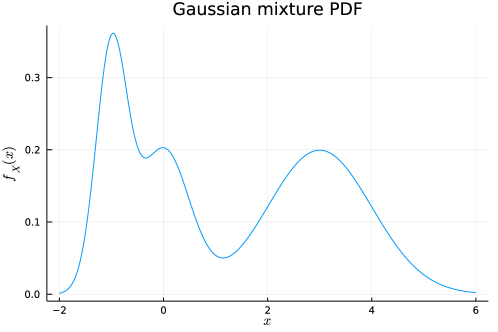
Figure 1: Example PDF of a univariate Gaussian mixture

Mixture models remain an active area of research and of development within Distributions.jl, estimation methods, and improved multivariate and matrix-variate support are planned for future releases. A more advanced example of estimation of a Gaussian mixture by a generic EM algorithm is presented in section D.4.

7 Applications of Distributions.jl

Distributions.jl has become a foundation for statistical programming in Julia, notably used for economic modeling (Federal Reserve Bank Of New York, 2019; Lyon et al., 2017), Markov chain Monte Carlo simulations (Smith, 2018) or randomized black-box optimization Feldt (2017) . We present below two applications of the package for non-parametric continuous density estimation and probabilistic programming.

7.1 Kernel density estimation

Probability density functions can be estimated in a non-parametric fashion using kernel density estimation (KDE, Rosenblatt, 1956; Parzen, 1962). This is supported through the KernelDensity.jl package, defining the kde function to infer an estimate density from data. Both univariate and bivariate density estimates are supported. Most of the algorithms and parameter selection heuristics developed in KernelDensity.jl are based on Silverman (2018). KernelDensity.jl supports multiple distributions as base kernels, and can be extended to other families. The default kernel used is Gaussian.

Example 7.1.

We highlight the estimation of a kernel density on data generated from the mixture of a log-normal and uniform distributions.

⬇

julia> import Random, Plots, KernelDensity

julia> using Distributions

julia> function generate_point(rng = Random.GLOBAL_RNG)

thres = rand(rng)

if thres >= 0.5

rand(rng, LogNormal())

else

rand(rng, Uniform(2.0, 3.0))

end

end

julia> mt = Random.MersenneTwister(42)

julia> xs = [generate_point(mt) for _ in 1:5000]

julia> bandwidths = [0.05, 0.1, 0.5]

julia> densities = [KernelDensity.kde(xs, bandwidth = bw) for bw in bandwidths]

julia> p = Plots.plot()

julia> for (b,d) in zip(bandwidths, densities)

Plots.plot!(p, d.x, d.density, labels = "bw = $b")

end

julia> Plots.xlims!(p, 0.0, 8.0)

julia> Plots.title!("KDE with Gaussian Kernel")

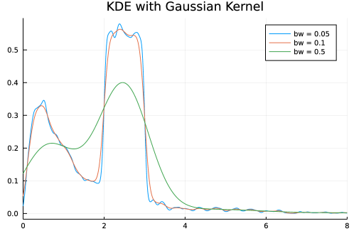
Figure 2: Adjusted KDE with various bandwidths

The bandwidth $bw=0.1$ seems not to overfit isolated data points without smoothing out important components. All examples provided use the Plots.jl package to plot results, which can be used with various plotting engines as back-end. We can compare the kernel density estimate to the real PDF as done in the following script and illustrated Figure 3.

⬇

julia> xvals = 0.01:0.01:8.0

julia> yvals = map(xvals) do x

comp1 = pdf(LogNormal(), x)

comp2 = pdf(Uniform(2.0, 3.0), x)

0.5 * comp1 + 0.5 * comp2

end

julia> p = Plots.plot(xvals, yvals, labels = "Real distribution")

julia> kde = KernelDensity.kde(xs, bandwidth = 0.1)

julia> Plots.plot!(p, kde.x, kde.density, labels = "KDE")

julia> Plots.plot!(p, xvals, yvals, labels = "Real distribution")

julia> Plots.xlims!(p, 0.0, 8.0)

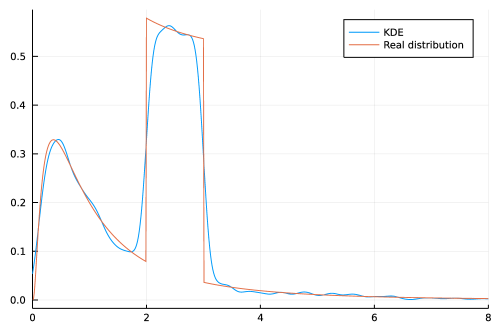
Figure 3: Comparison of the experimental and real PDF

The kernel density estimation technique relies on a base distribution (the kernel) which is convoluted against the data. The package uses directly the interface presented in section 4 to accept a Distribution as second parameter. The following script computes the kernel density estimates with a Gaussian and triangular distributions. The result is illustrated Figure 4.

⬇

julia> mt = Random.MersenneTwister(42)

julia> ($\mu$, $\sigma$) = (5.0, 1.0)

julia> xs = [rand(mt, Normal($\mu$, $\sigma$)) for _ in 1:50]

julia> ndist = Normal(0.0, 0.3)

julia> gkernel = kde(xs, ndist)

julia> tdist = TriangularDist(-0.5, 0.5)

julia> tkernel = KernelDensity.kde(xs, tdist)

julia> p = Plots.plot(tkernel.x, tkernel.density, labels = "Triangular kernel")

julia> Plots.plot!(p, gkernel.x, gkernel.density,

labels = "Gaussian kernel", legend = :left)

julia> Plots.title!(p, "Comparison of Gaussian and triangular kernels")

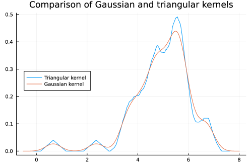
Figure 4: Comparison of different kernels defined as Distribution objects

The density estimator is computed via the Fourier transform: any distribution with a defined characteristic function (via the cf function from Distributions.jl) can be used as a kernel. The ability to manipulate distributions as types and objects allows end-users and package developers to compose on top of defined distributions and to define their own to use for kernel density estimations without any additional runtime cost. The kernel estimation of a bi-variate density is shown in D.2.

7.2 Probabilistic programming languages

Probabilistic programs are computer programs with the added capability of drawing the value of a variable from a probability distribution and conditioning variable values on observations (Gordon et al., 2014). They allow for the specification of complex relations between random variables using a set of constructs that go beyond typical graphical models to include flow control (e.g., loops, conditions), recursion, user-defined types and other algorithmic building blocks, differing from explicit graph construction by users, as done for instance in Smith (2018). Probabilistic programming languages (PPL) are programming language or libraries enabling developers to write such a probabilistic program. That is, they are a type of domain-specific language (DSL, Fowler, 2010). We refer the interested reader to Van de Meent et al. (2018) for an overview of PPL design and use, to Ścibior et al. (2017) for the analysis of Bayesian inference algorithms as transformations of intermediate representations, and to Vákár et al. (2019) for representation of recursive types in PPLs. They often fall in two categories.

In the first type, the PPL is its own independent language, including syntax and parsing, though it may rely on another ‘‘host’’ language for its execution engine. For example, Stan (Carpenter et al., 2017), uses its own .stan model specification format, though the parser and inference engine are written in C++. This type of approach benefits from defining its own syntax, thus designing it to look similar to the way equivalent statistical models are written. The model is also verified for syntactic correctness at compile-time.

In the second type of PPL, the language is embedded within and makes use of the syntax of the host language, leveraging that language’s native constructs. For example, PyMC (Patil et al., 2010; Kochurov et al., 2019), Pyro (Bingham et al., 2019), and Edward (Tran et al., 2016) all use Python as the host language, leveraging Theano, Torch, and TensorFlow, respectively, to perform many of the underlying inference computations. Here, the key advantage is that these PPLs gain access to the ecosystem of the host language (data structures, libraries, tooling). User documentation and development efforts can also focus on the key aspects of a PPL instead of the full stack.

However, both approaches to PPLs suffer from drawbacks. In the first type of PPLs, users must add new elements to their toolchains for the development and inference of statistical models. That is, they are likely to use a general-purpose programming language for other tasks, then switch to the PPL environment for the sampling and inference task, and then read the result back into the general-purpose programming language. One solution to this problem is to develop APIs in general purpose languages, but full inter-operability between two environments is non-trivial. Developers must then build a whole ecosystem around the PPL, including data structures, input/output, and text editor support, which costs time that might otherwise go toward improving the inference algorithms and optimization procedures.

While the second type of PPL may not require the development of a separate, parallel set of tools, it often runs into ‘‘impedance mismatches’’ of its own. In many cases, the host language has not been designed for a re-use of its constructs for probabilistic programming, resulting in syntax that aligns poorly with users’ mathematical intuitions. Moreover, duplication may still occur at the level of classes or libraries, as, for example, Pyro and Edward depend on Torch and TensorFlow, which replicate much of the linear algebra functionality of NumPy for their own array constructs.

By contrast, the design of Distributions.jl has enabled the development of embedded probabilistic programming languages such as Turing.jl (Ge et al., 2018), SOSS.jl (Scherrer, 2019), Omega.jl (Tavares, 2018) or Poirot.jl (Innes, 2019) with comparatively less overhead or friction with the host language. These PPLs are able to make use of three elements unique to the Julia ecosystem to challenge the dichotomy between embedded and stand-alone PPLs. First, they make use of Julia’s rich type system and multiple dispatch, which more easily support modeling mathematical constructs as types. Second, they all utilize Distributions.jl’s types and hierarchy for the sampling of random values and representation of their distributions. Finally, they use manipulations and transformations of the user Julia code to create new syntax that matches domain-specific requirements.

These transformations are either performed through macros (for Soss.jl and Turing.jl) or modifications of the compilation phases through compiler overdubbing (Omega.jl and Poirot.jl use Cassette.jl and IRTools.jl respectively to modify the user code or its intermediate representations). As in the Lisp tradition, Julia’s macros are written and manipulable in Julia itself and rewrite code during the lowering phase (Bezanson et al., 2018). Macros allow PPL designers to keep programs close to standard Julia while introducing package-specific syntax that more closely mimics statistical conventions, all without compromising on performance. For instance, a simple model definition from the Turing.jl documentation illustrates a model that is both readable as Julia code while staying close to statistical conventions:

⬇

julia> @model coinflip(y) = begin

p ~ Beta(1, 1)

N = length(y)

for n in 1:N

y[n] ~ Bernoulli(p)

end

end

With these syntax manipulation capabilities, along with compiled language performance, the combination of Julia with Distributions.jl provides an excellent foundation for further research and development of PPLs.

8 Conclusion and future work

We presented some of the types, structures and tools for modeling and computing on probability distributions in the JuliaStats ecosystem. The JuliaStats packages leverage some key constructs of Julia such as definition of new composite types, abstract parametric types and sub-typing, along with multiple dispatch. This allows users to express computations involving random number generation and the manipulation of probability distributions. A clear interface allows package developers to build new distributions from their mathematical definition. New algorithms can be developed, using the Distribution interface and as such extending the new features to all sub-types. These two features of Julia, namely extension of behavior to new types and definition of behavior over existing type hierarchy, allow different features built around the Distribution type to inter-operate seamlessly without hard coupling nor additional work from the package developers or end-users. Future work on the package will include the implementation of maximum likelihood estimation for other distributions, including mixtures and matrix-variate distributions.

Appendix A Installation of the relevant packages

The recommended installation of the relevant packages is done through the Pkg.jl tool available within the Julia distribution standard library. The common way to interact with the tool is within the REPL for Julia 1.0 and above. The closing square bracket "]" starts the pkg mode, in which the REPL stays until a return key is stroke.

julia> ] add StatsBase
(v1.0) pkg> add Distributions
(v1.0) pkg> add KernelDensity

This installation and all code snippets are guaranteed to work on Julia 1.0 and later with the semantic versioning commitment. Once installed, a package can be removed with the command rm PackageName or updated. All package modifications are guaranteed to respect version constraints for their direct and transitive dependencies. The packages StatsBase.jl, Distributions.jl, KernelDensity.jl are all open-source under the MIT license.

Appendix B Julia type system

B.1 Functions and methods

In Julia, a function ‘‘is an object that maps a tuple of argument values to a return value’’. A special case is an empty tuple as input, as in y = f(), and a function that returns the nothing value.

A function definition creates a top-level identifier with the function name. This can be passed around as any other value, for example to other functions. The function map takes a function and a collection map(f, c), and applies the function to each element of the collection to return the mapped values.

A function might represent a conceptual computation but different specific implementations might exist for this computation. For instance, the addition of two numbers is a common concept, but how it is implemented depends on the number type. The specific implementation of addition for complex numbers is

⬇

julia> +(z::Complex, w::Complex) = Complex(real(z) + real(w), imag(z) + imag(w))

This specific implementation is a method of the + function. Users can define their own implementation of existing functions, thus creating a new method for this function. Different methods can be implemented by changing the tuple of arguments, either with a different number of arguments or different types.

Example B.1.

In the following example, the function f has two methods. The function called depends on the number of arguments.

⬇

julia> function f(x)

println(x)

end

julia> function f(x, y)

println("x: $x & y: $y")

end

Example B.2.

In the following example, the function g has two methods. The first one is the most specific method and will be called for any type of the argument x that is a Number. Otherwise, the second method, which is less specific, will be called.

⬇

julia> g(x::T) where {T<:Number} = (3*x, x)

julia> g(x) = (x, 3)

Note that the order of definitions does not matter here, the least specific could have been defined first, and then the number-specialized implementation.

The method dispatched on by the Julia runtime is always the most specific.

Example B.3.

If there is no unique most specific method, Julia will raise a MethodError

⬇

julia> f(x, b::Float64) = x

f (generic function with 1 method)

julia> f(x::Float64, b) = b

f (generic function with 2 methods)

julia> f(3.0, 2.0)

ERROR: MethodError: f(::Float64, ::Float64) is ambiguous. Candidates:

f(x::Float64, b) in Main at REPL[2]:1

f(x, b::Float64) in Main at REPL[1]:1

Possible fix, define

f(::Float64, ::Float64)

B.2 Types

Julia enables users to define their own types including abstract types, mutable and immutable composite types or structures and primitive types (composed of bits). Packages often define abstract types to regroup types under one label and provide default implementation for a group of types. For examples, lots of methods require arguments which are identified as Number, upon which arithmetic operations can be applied, without having to re-define methods for each of the concrete number types. The most common type definition for end-users is composite types with the keyword struct as follows:

⬇

julia> struct S

field1::TypeOfField1

field2::TypeOfField2

field3 # a field without specified type will take the type 'Any'

end

In some cases, a type is defined for the sole purpose of creating a new method and does not require additional data in fields. The following definition is thus valid:

⬇

julia> struct S end

An instance of S is called a singleton, there is only one instance of such type.

Example B.4.

One use case is the specification of different algorithms for a procedure. The input of the procedure is always the same, so is the expected output, but different ways to compute the result are available.

⬇

julia> struct Alg1 end

julia> struct Alg2 end

julia> mul(x::Unsigned, y::Unsigned, ::Alg1) = x * y

julia> mul(x::T, y::Unsigned, ::Alg2) where {T<:Unsigned} = T(sum(x for _ in 1:y))

Note that in the second example, the information of the concrete type T of x is required to convert the sum expression into a number of type T.

Appendix C Comparison of Distributions.jl, Python/SciPy and R

In this section, we develop several comparative examples of how various computation tasks linked with probability distributions are performed using R, Python with SciPy/NumPy and Julia.

C.1 Sampling from various distributions

The following programs draw 100 samples from a Gamma distribution $\Gamma(k=10,\theta=2)$, in R:

⬇

R> set.seed(42)

R> rgamma(100, shape = 10, scale = 2)

The following Python version uses the NumPy & SciPy libraries.

⬇

>>> import numpy as np

>>> import scipy.stats as stats

>>> np.random.seed(42)

>>> stats.gamma.rvs(10, scale = 2, size = 100)

The following Julia version is written to stay close to the previous ones, thus setting the global seed and not passing along a new RNG object.

⬇

julia> import Random

julia> using Distributions

julia> Random.seed(42)

julia> g = Gamma(10, 2)

julia> rand(g, 100)

C.2 Representing a distribution with various scale parameters

The following code examples are in the same order as the previous sub-section:

⬇

R> x <- seq(-3.0,3.0,0.01)

R> y <- dnorm(x, mean = 0.5, sd = 0.75)

R> plot(x, y)

The Python example uses NumPy, SciPy and matplotlib.

⬇

>>> import numpy as np

>>> from scipy import stats

>>> from matplotlib import pyplot as plt

>>> x = np.arange(-3.0,3.0,0.01)

>>> y = stats.norm.pdf(x, loc = 0.5, scale = 0.75)

>>> plt.plot(x,y)

The Julia version uses defines a Gaussian random variable object n:

⬇

julia> using Distributions

julia> using Plots

julia> n = Normal(0.5, 0.75)

julia> x = -3.0:0.01:3.0

julia> y = pdf.(n, x)

julia> plot(x, y)

Note that unlike the R and Python examples, x does not need to be represented as an array but as an iterable not storing all intermediate values, saving time and memory. The dot or broadcast operator in pdf.(n, x) applies the function to all elements of x.

Appendix D Wine data analysis

In this section, we show the example of analyses run on the wine dataset Aeberhard et al. (1994) obtained on the UCI machine learning repository. The data can be fetched directly over HTTP from within Julia.

⬇

julia> using Distributions, DelimitedFiles

julia> import Plots

julia> wine_data_url =

"https://archive.ics.uci.edu/ml/machine-learning-databases/wine/wine.data"

julia> wine_data_file = download(wine_data_url)

julia> raw_wine_data = readdlm(wine_data_file, ',', Float64)

julia> wine_quant = raw_wine_data[:,2:end]

julia> wine_labels = Int.(raw_wine_data[:,1])

D.1 Automatic multivariate fitting

We can then fit a multivariate distribution to some variables and observe the result:

⬇

julia> alcohol = wine_quant[:,1]

julia> log_malic_acid = log.(wine_quant[:,2])

julia> obs = permutedims([alcohol log_malic_acid])

julia> res_normal = fit_mle(MvNormal, obs)

julia> cont_func(x1, x2) = pdf(res_normal, [x1,x2])

julia> p = Plots.contour(11.0:0.05:15.0, -0.5:0.05:2.5, cont_func)

julia> Plots.scatter!(p, alcohol, log_malic_acid, label="Data points")

julia> Plots.title!(

p, "Wine scatter plot & Gaussian maximum likelihood estimation")

Note that fit_mle needs observations as columns, hence the use of permutedims.

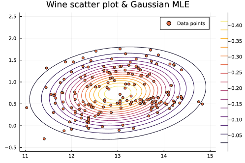
Figure 5: Multivariate Gaussian MLE over $(x_{1},x_{2})$ of the wine data

D.2 Non-parametric density estimation

Assuming a multivariate Gaussian distribution might be considered a too strong assumption, a kernel density estimator can be used on the same data:

⬇

julia> wine_kde = KernelDensity.kde((alcohol, log_malic_acid))

julia> cont_kde(x1, x2) = pdf(wine_kde, x1, x2)

julia> p = Plots.contour(11.0:0.05:15.0, -0.5:0.05:2.5, cont_kde)

julia> Plots.scatter!(p, alcohol, log_malic_acid, group=wine_labels)

julia> Plots.title!(p, "Wine scatter plot & Kernel Density Estimation")

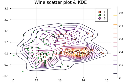
Figure 6: KDE over $(x_{1},x_{2})$ of the wine data

The resulting kernel density estimation is shown Figure 6. The level curves highlight the centers of the three classes of the dataset.

D.3 Product distribution model

Given that a logarithmic transform was used for $x_{2}$, a shifted log-normal distribution can be fitted: $X_{2}-0.73\sim LogNormal(\mu,\sigma)$. The maximum likelihood estimator could be computed as in section D.1. Instead, we will demonstrate the simplicity of building new constructs and optimize over them. A Product distribution is implemented in Distributions.jl, defining a Cartesian product of the two variables, thus assuming their independence:

$$X=(X_{1},X_{2})$$ (1)

Assuming $X_{1}$ follows a normal distribution, given a vector of 4 parameters $\left[\mu_{1},\sigma_{1},\mu_{2},\sigma_{2}\right]$, the distribution can be constructed:

⬇

julia> function build_product_distribution(p)

return product_distribution([

Normal(p[1], p[2]),

LogNormal(p[3], p[4]),

])

end

Computing the log-likelihood of a product distribution boils down to the sum of the individual log-likelihood. The gradient could be computed analytically but automatic differentiation will be leveraged here using ForwardDiff.jl (Revels et al., 2016):

⬇

julia> function loglike(p)

d = build_product_distribution(p)

return loglikelihood(d.v[1], wine_quant[:,1]) +

loglikelihood(d.v[2], wine_quant[:,2] .- 0.73)

end

julia> $\nabla$L(p) = ForwardDiff.gradient(loglike, p)

Once the gradient obtained, first-order optimization methods can be applied. To keep everything self-contained, a gradient descent with decreasing step will be applied:

$$x_{k+1}=x_{k}+\rho_{k}\nabla\mathcal{L}(x_{k})$$ (2)

$$\rho_{k+1}=\rho_{0}/(k+m)$$ (3)

With $(\rho_{0},m)$ constants.

⬇

julia> p = [10.0 + 3.0 * rand(), rand()+1, 2.0 + 3.0*rand(), rand()+1]

julia> iter = 1

julia> maxiter = 5000

julia> while iter <= maxiter && sum(abs.($\nabla$L(p))) >= 10^-6

p = p + 0.05 * inv(iter+5) * $\nabla$L(p)

p[2] = p[2] < 0 ? -p[2] : p[2]

p[4] = p[4] < 0 ? -p[4] : p[4]

iter += 1

end

julia> d = build_product_distribution(p)

Without further code or method tuning, the optimization takes about $590\mu s$ and few iterations to converge as shown Figure 8. For more complex use cases, users would look at more sophisticated techniques as developed in JuliaSmoothOptimizers (Orban and Siqueira, 2019) or Optim.jl (Mogensen and Riseth, 2018). Figure 7 highlights the resulting marginal and joint distributions.

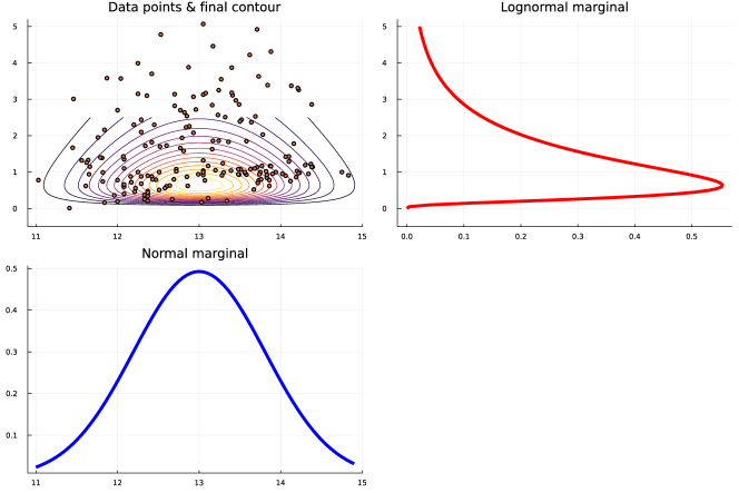
Figure 7: Resulting inferred joint and marginal distribution for $(X_{1},X_{2})$

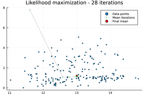
Figure 8: Illustration of the likelihood maximization convergence

D.4 Implementation of an Expectation-Maximization algorithm

In this section, we highlight how Julia dispatch mechanism and Distributions.jl type hierarchy can help users define algorithms in a generic fashion, leveraging specific structure but allowing their extension. We know that the observations from the wine data set are split into different classes $Z$. We will consider only the two first variables, with the second at a log-scale: $X=(x_{1},log(x2))$.

The expectation step computes the probability for each observation $i$ to belong to each label $k$:

⬇

julia> function expectation_step(X, dists, prior)

n = size(X, 1)

Z = Matrix{Float64}(undef, n, length(prior))

for k in eachindex(prior)

for i in 1:n

Z[i,k] = prior[k] * pdf(dists[k], X[i,:]) /

sum(

prior[j] * pdf(dists[j], X[i,:])

for j in eachindex(prior)

)

end

end

return Z

end

dists is a vector of distributions, note that no assumption is needed on these distributions, other than the standard interface. The only computation applied is indeed the computation of the pdf for each of these.

The operation for which the specific structure of the distribution is required is the maximization step. For many distributions, a closed-form solution of the maximum-likelihood estimator is known, avoiding expensive optimization schemes as developed in D.3. In the case of the Normal distribution, the maximum likelihood estimator is given by the empirical mean and covariance matrix. We define the function maximization_step to take a distribution type, the data X and current label estimates $Z$, computing both the prior probabilities of each of the classes $\pi_{k}$ and the corresponding conditional distribution $D_{k}$, it returns the pair of vectors $(D,\pi)$.

⬇

julia> function maximization_step(::Type{<:MvNormal}, X, Z)

n = size(X, 1)

Nk = size(Z, 2)

$\mu$ = map(1:Nk) do k

num = sum(Z[i,k] .* X[i,:] for i in 1:n)

den = sum(Z[i,k] for i in 1:n)

num / den

end

$\Sigma$ = map(1:Nk) do k

num = zeros(size(X, 2), size(X, 2))

for i in 1:n

r = X[i,:] .- $\mu$[k]

num .= num .+ Z[i,k] .* (r * r')

end

den = sum(Z[i,k] for i in 1:n)

num ./ den

end

prior = [inv(n) * sum(Z[i,k] for i in 1:n)

for k in 1:Nk

]

dists = map(1:Nk) do k

MvNormal($\mu$[k], $\Sigma$[k] + 10e-7I)

end

return (dists, prior)

end

The final block is a function alternatively computing $Z$ and $(D,\pi)$ until convergence:

⬇

julia> function expectation_maximization(

D::Type{<:Distribution},

X, Nk,

maxiter = 500,

loglike_diff = 10e-5)

# initialize classes

n = size(X,1)

Z = zeros(n, Nk)

for i in 1:n

j0 = mod(i,Nk)+1

j1 = j0 > 1 ? j0-1 : 2

Z[i,j0] = 0.75

Z[i,j1] = 0.25

end

(dists, prior) = maximization_step(D, X, Z)

l = loglike_mixture(X, dists, prior)

lprev = 0.0

iter = 0

# EM iterations

while iter < maxiter && abs(lprev-l) > loglike_diff

Z = expectation_step(X, dists, prior)

(dists, prior) = maximization_step(D, X, Z)

lprev = l

l = loglike_mixture(X, dists, prior)

iter += 1

end

return (dists, prior, Z, l, iter)

end

julia> function loglike_mixture(X, dists, prior)

l = zero(eltype(X))

n = size(X,1)

for i in 1:n

l += log(

sum(prior[k] * pdf(dists[k], X[i,:]) for k in eachindex(prior))

)

end

return l

end

Starting from an alternated affectation of observations to labels, it calls the two methods defined above for the E and M steps.

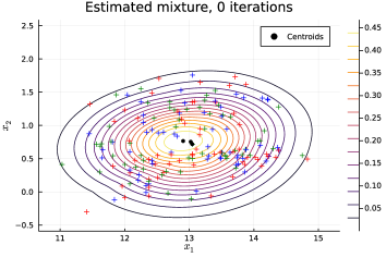
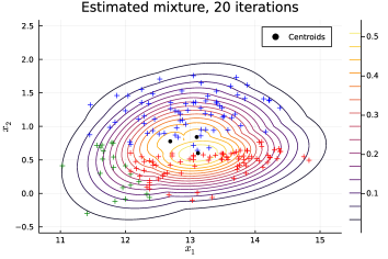
$n=0$	$n=20$
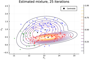
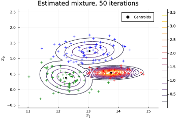
$n=25$	$n=50$

Figure 9: Convergence of the EM algorithm

The strength of this implementation is that extending it to more functions only requires to implement maximization_step(D, X, Z) for the new distribution. The rest of the structure will then work as expected.

Appendix E Benchmarks on mixture PDF evaluations

In this section, we evaluate the computation time for the PDF of mixtures of distributions, on mixture of Gaussian univariate distributions, and then on a mixture of heterogeneous distributions including normal and log-normal distributions.

⬇

julia> using BenchmarkTools: @btime

julia> distributions = [

Normal(-1.0, 0.3),

Normal(0.0, 0.5),

Normal(3.0, 1.0),

]

julia> priors = [0.25, 0.25, 0.5]

julia> gmm_normal = MixtureModel(distributions, priors)

julia> x = rand()

julia> @btime pdf($gmm_normal, $x)

julia> large_normals = [Normal(rand(), rand()) for _ in 1:1000]

julia> large_probs = [rand() for _ in 1:1000]

julia> large_probs .= large_probs ./ sum(large_probs)

julia> gmm_large = MixtureModel(large_normals, large_probs)

@btime pdf($gmm_large, $x)

julia> large_h = append!(

ContinuousUnivariateDistribution[Normal(rand(), rand()) for _ in 1:1000],

ContinuousUnivariateDistribution[LogNormal(rand(), rand()) for _ in 1:1000],

)

julia> large_h_probs = [rand() for _ in 1:2000]

julia> large_h_probs .= large_h_probs ./ sum(large_h_probs)

julia> gmm_h = MixtureModel(large_h, large_h_probs)

julia> @btime pdf($gmm_h, $x)

The PDF computation on the small, large and heterogeneous mixture take on average $332ns$, $105\mu s$ and $259\mu s$ respectively. We also compare the computation time with the manual computation of the mixture evaluated as such:

⬇

julia> function manual_computation(mixture, x)

v = zero(eltype(mixture))

p = probs(mixture)

d = components(mixture)

for i in 1:ncomponents(mixture)

if p[i] > 0

v += p[i] * pdf(d[i], x)

end

end

return v

end

The PDF computation currently in the library is faster than the manual one, the sum over weighted PDF of the components being performed without branching. The ratio of manual time over the implementation of Distributions.jl being on average 1.24, 5.88 and 1.28 respectively. The greatest acceleration is observed for large mixtures with homogeneous component types. The slow-down for heterogeneous component types is due to the compiler not able to infer the type of each element of the mixture, thus replacing static with dynamic dispatch. The Distributions.jl package also contains a /perf folder containing experiments on performance to track possible regressions and compare different implementations.

References

- Aeberhard et al. (1994) Aeberhard S, Coomans D, De Vel O (1994). ‘‘Comparative Analysis of Statistical Pattern Recognition Methods in High Dimensional Settings.’’ Pattern Recognition, 27(8), 1065--1077. 10.1016/0031-3203(94)90145-7.
- Ahrens and Dieter (1982) Ahrens JH, Dieter U (1982). ‘‘Computer Generation of Poisson Deviates from Modified Normal Distributions.’’ ACM Transactions on Mathematical Software, 8(2), 163--179. 10.1145/355993.355997.
- Aldrich (1997) Aldrich J (1997). ‘‘R.A. Fisher and the Making of Maximum Likelihood 1912--1922.’’ Statistical Science, 12(3), 162--176. 10.1214/ss/1030037906.
- Bezanson et al. (2018) Bezanson J, Chen J, Chung B, Karpinski S, Shah VB, Vitek J, Zoubritzky L (2018). ‘‘\proglangJulia: Dynamism and Performance Reconciled by Design.’’ Proceedings of the ACM on Programming Languages, 2(OOPSLA), 120. 10.1145/3276490.
- Bezanson et al. (2017) Bezanson J, Edelman A, Karpinski S, Shah V (2017). ‘‘\proglangJulia: A Fresh Approach to Numerical Computing.’’ SIAM Review, 59(1), 65--98. 10.1137/141000671.
- Bingham et al. (2019) Bingham E, Chen JP, Jankowiak M, Obermeyer F, Pradhan N, Karaletsos T, Singh R, Szerlip P, Horsfall P, Goodman ND (2019). ‘‘\pkgPyro: Deep Universal Probabilistic Programming.’’ The Journal of Machine Learning Research, 20(1), 973--978.
- \pkgBoost Developers (2018) \pkgBoost Developers (2018). ‘‘\pkgBoost \proglangC++ Libraries.’’ URL https://www.boost.org/.
- Carpenter et al. (2017) Carpenter B, Gelman A, Hoffman MD, Lee D, Goodrich B, Betancourt M, Brubaker M, Guo J, Li P, Riddell A (2017). ‘‘\proglangStan: A Probabilistic Programming Language.’’ Journal of Statistical Software, 76(1), 1--32. 10.18637/jss.v076.i01.
- Devroye (1986) Devroye L (1986). Non-Uniform Random Variate Generation. Springer-Verlag, New York.
- Duncan (2020) Duncan J (2020). ‘‘Model building of golf putting with \proglangTuring.jl.’’ URL https://web.archive.org/web/20210611145623/https://jduncstats.com/posts/2019-11-02-golf-turing/.
- Erwig and Kollmansberger (2006) Erwig M, Kollmansberger S (2006). ‘‘Functional Pearls: Probabilistic Functional Programming in \proglangHaskell.’’ Journal of Functional Programming, 16(1), 21--34. 10.1017/s0956796805005721.
- Federal Reserve Bank Of New York (2019) Federal Reserve Bank Of New York (2019). ‘‘\pkgDSGE.jl: Solve and Estimate Dynamic Stochastic General Equilibrium Models (Including the New York Fed DSGE).’’ URL https://github.com/FRBNY-DSGE/DSGE.jl.
- Feldt (2017) Feldt R (2017). ‘‘\pkgBlackBoxOptim.jl.’’ URL https://github.com/robertfeldt/BlackBoxOptim.jl.
- Fowler (2010) Fowler M (2010). Domain-Specific Languages. Pearson Education.
- Ge et al. (2018) Ge H, Xu K, Ghahramani Z (2018). ‘‘\proglangTuring: Composable Inference for Probabilistic Programming.’’ In Proceedings of the Twenty-First International Conference on Artificial Intelligence and Statistics, pp. 1682--1690. URL http://proceedings.mlr.press/v84/ge18b.html.
- Gelman (2019) Gelman A (2019). ‘‘Model Building and Expansion for Golf Putting (accessed June 2021).’’ URL https://mc-stan.org/users/documentation/case-studies/golf.html.
- Gordon et al. (2014) Gordon AD, Henzinger TA, Nori AV, Rajamani SK (2014). ‘‘Probabilistic Programming.’’ In Proceedings of the on Future of Software Engineering, pp. 167--181. ACM.
- Innes (2019) Innes M (2019). ‘‘\pkgPoirot.jl.’’ Version 0.1, URL https://github.com/MikeInnes/Poirot.jl.
- JuliaStats (2019) JuliaStats (2019). ‘‘\pkgDistributions.jl.’’ 10.5281/zenodo.2647458.
- Kiselyov and Shan (2009) Kiselyov O, Shan CC (2009). ‘‘Embedded Probabilistic Programming.’’ In WM Taha (ed.), Domain-Specific Languages, pp. 360--384. Springer-Verlag, Berlin.
- Kochurov et al. (2019) Kochurov M, Carroll C, Wiecki T, Lao J (2019). ‘‘\pkgPyMC4: Exploiting Coroutines for Implementing a Probabilistic Programming Framework.’’ URL https://openreview.net/forum?id=rkgzj5Za8H.
- Le Goc and Donzé (2015) Le Goc Y, Donzé A (2015). ‘‘\pkgEVL: A Framework for Multi-Methods in \proglangC++.’’ Science of Computer Programming, 98, 531--550. ISSN 0167-6423. 10.1016/j.scico.2014.08.003.
- Lyon et al. (2017) Lyon S, Sargent TJ, Stachurski J (2017). ‘‘\pkgQuantEcon.jl.’’ URL https://github.com/QuantEcon/QuantEcon.jl.
- Matsumoto and Nishimura (1998) Matsumoto M, Nishimura T (1998). ‘‘Mersenne Twister: A 623-Dimensionally Equidistributed Uniform Pseudo-Random Number Generator.’’ ACM Transactions on Modeling and Computer Simulation, 8(1), 3--30. 10.1145/272991.272995.
- Mogensen and Riseth (2018) Mogensen PK, Riseth AN (2018). ‘‘\pkgOptim: A Mathematical Optimization Package for \proglangJulia.’’ Journal of Open Source Software, 3(24), 615. 10.21105/joss.00615.
- Orban and Siqueira (2019) Orban D, Siqueira AS (2019). ‘‘\pkgJuliaSmoothOptimizers: Infrastructure and Solvers for Continuous Optimization in \proglangJulia.’’ 10.5281/zenodo.2655082.
- Parzen (1962) Parzen E (1962). ‘‘On Estimation of a Probability Density Function and Mode.’’ The Annals of Mathematical Statistics, 33(3), 1065--1076. 10.1214/aoms/1177704472.
- Patil et al. (2010) Patil A, Huard D, Fonnesbeck C (2010). ‘‘\pkgPyMC: Bayesian Stochastic Modelling in \proglangPython.’’ Journal of Statistical Software, 35(4), 1--81. 10.18637/jss.v035.i04.
- Pham and Garat (1997) Pham DT, Garat P (1997). ‘‘Blind Separation of Mixture of Independent Sources through a Quasi-Maximum Likelihood Approach.’’ IEEE Transactions on Signal Processing, 45(7), 1712--1725. 10.1109/78.599941.
- Pirkelbauer et al. (2010) Pirkelbauer P, Solodkyy Y, Stroustrup B (2010). ‘‘Design and Evaluation of \proglangC++ Open Multi-Methods.’’ Science of Computer Programming, 75(7), 638--667. 10.1016/j.scico.2009.06.002. Generative Programming and Component Engineering (GPCE 2007).
- \pkgPyMC (2019) \pkgPyMC (2019). ‘‘Model building and expansion for golf putting.’’ URL http://web.archive.org/web/20191210110708/https://nbviewer.jupyter.org/github/pymc-devs/pymc3/blob/master/docs/source/notebooks/putting_workflow.ipynb.
- Revels et al. (2016) Revels J, Lubin M, Papamarkou T (2016). ‘‘Forward-Mode Automatic Differentiation in \proglangJulia.’’ arXiv 1607.07892, arXiv.org E-Print Archive. URL https://arxiv.org/abs/1607.07892.
- Rosenblatt (1956) Rosenblatt M (1956). ‘‘Remarks on Some Nonparametric Estimates of a Density Function.’’ The Annals of Mathematical Statistics, 27(3), 832--837. 10.1214/aoms/1177728190.
- Ruckdeschel et al. (2006) Ruckdeschel P, Kohl M, Stabla T, Camphausen F (2006). ‘‘\proglangS4 Classes for Distributions.’’ \proglangR News, 6(2), 2--6.
- Schauer (2018) Schauer M (2018). ‘‘\pkgBridge.jl: a Statistical Toolbox for Diffusion Processes and Stochastic Differential Equations.’’ 10.5281/zenodo.891230. Version 0.9.
- Scherrer (2019) Scherrer C (2019). ‘‘\pkgSoss.jl: Probabilistic Programming via Source Rewriting.’’ Version 0.1, URL https://github.com/cscherrer/Soss.jl.
- Ścibior et al. (2015) Ścibior A, Ghahramani Z, Gordon AD (2015). ‘‘Practical Probabilistic Programming with Monads.’’ ACM SIGPLAN Notices, 50(12), 165--176. 10.1145/2887747.2804317.
- Ścibior et al. (2017) Ścibior A, Kammar O, Vákár M, Staton S, Yang H, Cai Y, Ostermann K, Moss SK, Heunen C, Ghahramani Z (2017). ‘‘Denotational Validation of Higher-Order Bayesian Inference.’’ Proceedings of the ACM on Programming Languages, 2, 60. 10.1145/3158148.
- Silverman (2018) Silverman BW (2018). Density Estimation for Statistics and Data Analysis. Routledge.
- Smith (2018) Smith BJ (2018). ‘‘\pkgMamba.jl: Markov Chain Monte Carlo (MCMC) for Bayesian Analysis in \proglangJulia.’’ Version 0.12, URL https://github.com/brian-j-smith/Mamba.jl.
- Tavares (2018) Tavares Z (2018). ‘‘\pkgOmega.jl: Causal, Higher-Order, Probabilistic Programming.’’ Version 0.1, URL https://github.com/zenna/Omega.jl.
- Tran et al. (2016) Tran D, Kucukelbir A, Dieng AB, Rudolph M, Liang D, Blei DM (2016). ‘‘\pkgEdward: A Library for Probabilistic Modeling, Inference, and Criticism.’’ arXiv 1610.09787, arXiv.org E-Print Archive. URL https://arxiv.org/abs/1610.09787.
- Vákár et al. (2019) Vákár M, Kammar O, Staton S (2019). ‘‘A Domain Theory for Statistical Probabilistic Programming.’’ Proceedings of the ACM on Programming Languages, 3(POPL), 36. 10.1145/3290349.
- Van de Meent et al. (2018) Van de Meent JW, Paige B, Yang H, Wood F (2018). ‘‘An Introduction to Probabilistic Programming.’’ arXiv 1809.10756, arXiv.org E-Print Archive. URL https://arxiv.org/abs/1809.10756.
- Virtanen et al. (2020) Virtanen P, Gommers R, Oliphant TE, Haberland M, Reddy T, Cournapeau D, Burovski E, Peterson P, Weckesser W, Bright J, van der Walt SJ, Brett M, Wilson J, Millman KJ, Mayorov N, Nelson ARJ, Jones E, Kern R, Larson E, Carey CJ, Polat İ, Feng Y, Moore EW, VanderPlas J, Laxalde D, Perktold J, Cimrman R, Henriksen I, Quintero EA, Harris CR, Archibald AM, Ribeiro AH, Pedregosa F, van Mulbregt P, SciPy 10 Contributors (2020). ‘‘\pkgSciPy 1.0: Fundamental Algorithms for Scientific Computing in \proglangPython.’’ Nature Methods, 17, 261--272. 10.1038/s41592-019-0686-2.
- Wilks (1938) Wilks SS (1938). ‘‘The Large-Sample Distribution of the Likelihood Ratio for Testing Composite Hypotheses.’’ The Annals of Mathematical Statistics, 9(1), 60--62. 10.1214/aoms/1177732360.
- Zappa Nardelli et al. (2018) Zappa Nardelli F, Belyakova J, Pelenitsyn A, Chung B, Bezanson J, Vitek J (2018). ‘‘\proglangJulia Subtyping: A Rational Reconstruction.’’ Proceedings of the ACM on Programming Languages, 2(OOPSLA), 113. 10.1145/3276483.