Parallel Algorithms for Butterfly Computations

Abstract

Butterflies are the smallest non-trivial subgraph in bipartite graphs, and therefore having efficient computations for analyzing them is crucial to improving the quality of certain applications on bipartite graphs. In this paper, we design a framework called ParButterfly that contains new parallel algorithms for the following problems on processing butterflies: global counting, per-vertex counting, per-edge counting, tip decomposition (vertex peeling), and wing decomposition (edge peeling). The main component of these algorithms is aggregating wedges incident on subsets of vertices, and our framework supports different methods for wedge aggregation, including sorting, hashing, histogramming, and batching. In addition, ParButterfly supports different ways of ranking the vertices to speed up counting, including side ordering, approximate and exact degree ordering, and approximate and exact complement coreness ordering. For counting, ParButterfly also supports both exact computation as well as approximate computation via graph sparsification. We prove strong theoretical guarantees on the work and span of the algorithms in ParButterfly.

We perform a comprehensive evaluation of all of the algorithms in ParButterfly on a collection of real-world bipartite graphs using a 48-core machine. Our counting algorithms obtain significant parallel speedup, outperforming the fastest sequential algorithms by up to 13.6x with a self-relative speedup of up to 38.5x. Compared to general subgraph counting solutions, we are orders of magnitude faster. Our peeling algorithms achieve self-relative speedups of up to 10.7x and outperform the fastest sequential baseline by up to several orders of magnitude.

This is an extended version of the paper of the same name that appeared in the SIAM Symposium on Algorithmic Principles of Computer Systems, 2020 [56].

1 Introduction

A fundamental problem in large-scale network analysis is finding and enumerating basic graph motifs. Graph motifs that represent the building blocks of certain networks can reveal the underlying structures of these networks. Importantly, triangles are core substructures in unipartite graphs, and indeed, triangle counting is a key metric that is widely applicable in areas including social network analysis [45], spam and fraud detection [8], and link classification and recommendation [62]. However, many real-world graphs are bipartite and model the affiliations between two groups. For example, bipartite graphs are used to represent peer-to-peer exchange networks (linking peers to the data they request), group membership networks (e.g., linking actors to movies they acted in), recommendation systems (linking users to items they rated), factor graphs for error-correcting codes, and hypergraphs [12, 39]. Bipartite graphs contain no triangles; the smallest non-trivial subgraph is a butterfly (also known as rectangles), which is a $(2,2)$-biclique (containing two vertices on each side and all four possible edges among them), and thus having efficient algorithms for counting butterflies is crucial for applications on bipartite graphs [64, 5, 53]. Notably, butterfly counting has applications in link spam detection [24] and document clustering [18]. Moreover, butterfly counting naturally lends itself to finding dense subgraph structures in bipartite networks. Zou [71] and Sariyüce and Pinar [54] developed peeling algorithms to hierarchically discover dense subgraphs, similar to the $k$-core decomposition for unipartite graphs [55, 43]. An example bipartite graph and its butterflies is shown in Figure 1.

There has been recent work on designing efficient sequential algorithms for butterfly counting and peeling [14, 64, 70, 71, 53, 54, 66]. However, given the high computational requirements of butterfly computations, it is natural to study whether we can obtain performance improvements using parallel machines. This paper presents a framework for butterfly computations, called ParButterfly, that enables us to obtain new parallel algorithms for butterfly counting and peeling. ParButterfly is a modular framework that enables us to easily experiment with many variations of our algorithms. We not only show that our algorithms are efficient in practice, but also prove strong theoretical bounds on their work and span. Given that all real-world bipartite graphs fit on a multicore machine, we design parallel algorithms for this setting.

Figure 1: The butterflies in this graph are $\{u_{1},v_{1},u_{2},v_{2}\}$, $\{u_{1},v_{1},u_{2},v_{3}\}$, and $\{u_{1},v_{2},u_{2},v_{3}\}$. The red, blue, and green edges each produce a wedge ($\{u_{1},v_{1},u_{2}\}$, $\{u_{1},v_{2},u_{2}\}$, and $\{u_{1},v_{3},u_{2}\}$). Note that these wedges all share the same endpoints, namely $u_{1}$ and $u_{2}$. Thus, any combination of two of these wedges forms a butterfly. For example, $\{u_{1},v_{1},u_{2}\}$ and $\{u_{1},v_{2},u_{2}\}$ combine to form a butterfly $\{u_{1},v_{1},u_{2},v_{2}\}$. However, the dashed edges produce another wedge, $\{u_{2},v_{3},u_{3}\}$, which has different endpoints, namely $u_{2}$ and $u_{3}$. This wedge cannot be combined with any of the previous wedges to form a butterfly.

For butterfly counting, the main procedure involves finding wedges ($2$-paths) and combining them to count butterflies. See Figure 1 for an example of wedges. In particular, we want to find all wedges originating from each vertex, and then aggregate the counts of wedges incident to every distinct pair of vertices forming the endpoints of the wedge. With these counts, we can obtain global, per-vertex, and per-edge butterfly counts. The ParButterfly framework provides different ways to aggregate wedges in parallel, including sorting, hashing, histogramming, and batching. Also, we can speed up butterfly counting by ranking vertices and only considering wedges formed by a particular ordering of the vertices. ParButterfly supports different parallel ranking methods, including side-ordering, approximate and exact degree-ordering, and approximate and exact complement-coreness ordering. These orderings can be used with any of the aggregation methods. To further speed up computations on large graphs, ParButterfly also supports parallel approximate butterfly counting via graph sparsification based on ideas by Sanei-Mehri et al. [53] for the sequential setting. Furthermore, we integrate into ParButterfly a recently proposed cache optimization for butterfly counting by Wang et al. [65].

In addition, ParButterfly provides parallel algorithms for peeling bipartite networks based on sequential dense subgraph discovery algorithms developed by Zou [71] and Sariyüce and Pinar [54]. Our peeling algorithms iteratively remove the vertices (tip decomposition) or edges (wing decomposition) with the lowest butterfly count until the graph is empty. Each iteration removes vertices (edges) from the graph in parallel and updates the butterfly counts of neighboring vertices (edges) using the parallel wedge aggregation techniques that we developed for counting. We use a parallel bucketing data structure by Dhulipala et al. [19] and a new parallel Fibonacci heap to efficiently maintain the butterfly counts.

We prove theoretical bounds showing that some variants of our counting and peeling algorithms are highly parallel and match the work of the best sequential algorithm. For a graph $G(V,E)$ with $m$ edges and arboricity $\alpha$, ParButterfly gives a counting algorithm that takes $\operatorname{O}\bigl{(}\alpha m\bigr{)}$ expected work, $\operatorname{O}\bigl{(}\log m\bigr{)}$ span with high probability (w.h.p.), and $\operatorname{O}\bigl{(}\min(n^{2},\alpha m)\bigr{)}$ additional space. Moreover, we design a parallel Fibonacci heap that improves upon the work bounds for vertex-peeling from Sariyüce and Pinar’s sequential algorithms, which take work proportional to the maximum number of per-vertex butterflies. ParButterfly gives a vertex-peeling algorithm that takes $\operatorname{O}\bigl{(}\min({\text{max-b}}_{v},\allowbreak\rho_{v}\log n)+\allowbreak\sum_{v\in V}\text{deg}(v)^{2}\bigr{)}$ expected work, $\operatorname{O}\bigl{(}\rho_{v}\log^{2}n\bigr{)}$ span w.h.p., and $\operatorname{O}\bigl{(}n^{2}+\allowbreak{\text{max-b}}_{v}\bigr{)}$ additional space, and an edge-peeling algorithm that takes $\operatorname{O}\bigl{(}\min({\text{max-b}}_{e},\allowbreak\rho_{e}\log n)+\sum_{(u,v)\in E}\sum_{u^{\prime}\in N(v)}\min(\text{deg}(u),\allowbreak\text{deg}(u^{\prime}))\bigr{)}$ expected work, $\operatorname{O}\bigl{(}\rho_{e}\log^{2}m\bigr{)}$ span w.h.p., and $\operatorname{O}\bigl{(}m+\allowbreak{\text{max-b}}_{e}\bigr{)}$ additional space, where $\text{max-b}_{v}$ and $\text{max-b}_{e}$ are the maximum number of per-vertex and per-edge butterflies and $\rho_{v}$ and $\rho_{e}$ are the number of vertex and edge peeling iterations required to remove the entire graph. Additionally, given a slightly relaxed work bound, we can improve the space bounds in both algorithms; specifically, we have a vertex-peeling algorithm that takes $\operatorname{O}\bigl{(}\rho_{v}\log n+\allowbreak\sum_{v\in V}\text{deg}(v)^{2}\bigr{)}$ expected work, $\operatorname{O}\bigl{(}\rho_{v}\log^{2}n\bigr{)}$ span w.h.p., and $\operatorname{O}\bigl{(}n^{2}\bigr{)}$ additional space, and we have an edge-peeling algorithm that takes $\operatorname{O}\bigl{(}\rho_{e}\log n+\sum_{(u,v)\in E}\sum_{u^{\prime}\in N(v)}\min(\text{deg}(u),\allowbreak\text{deg}(u^{\prime}))\bigr{)}$ expected work, $\operatorname{O}\bigl{(}\rho_{e}\log^{2}m\bigr{)}$ span w.h.p., and $\operatorname{O}\bigl{(}m\bigr{)}$ additional space.

Moreover, we demonstrate further work-space tradeoffs with a vertex-peeling algorithm that takes $\operatorname{O}\bigl{(}\rho_{v}\log n\allowbreak+b\bigr{)}$ expected work, $\operatorname{O}\bigl{(}\rho_{v}\log^{2}n\bigr{)}$ span w.h.p., and $\operatorname{O}\bigl{(}\alpha m\bigr{)}$ additional space, where $b$ is the total number of butterflies. Similarly, we give an edge-peeling algorithm that takes $\operatorname{O}\bigl{(}\rho_{e}\log n\allowbreak+b\bigr{)}$ expected work, $\operatorname{O}\bigl{(}\rho_{e}\log^{2}n\bigr{)}$ span w.h.p., and $\operatorname{O}\bigl{(}\alpha m\bigr{)}$ additional space. We can improve the work complexities to $\operatorname{O}\bigl{(}b\bigr{)}$ expected work by allowing $\operatorname{O}\bigl{(}\alpha m+\allowbreak{\text{max-b}}_{v}\bigr{)}$ and $\operatorname{O}\bigl{(}\alpha m+\allowbreak{\text{max-b}}_{e}\bigr{)}$ additional space for vertex-peeling and edge-peeling respectively.

We present a comprehensive experimental evaluation of all of the different variants of counting and peeling algorithms in the ParButterfly framework. On a 48-core machine, our counting algorithms achieve self-relative speedups of up to 38.5x and outperform the fastest sequential baseline by up to 13.6x. Our peeling algorithms achieve self-relative speedups of up to 10.7x and due to their improved work complexities, outperform the fastest sequential baseline by up to several orders of magnitude. Compared to PGD [2], a state-of-the-art parallel subgraph counting solution that can be used for butterfly counting as a special case, we are 349.6–5169x faster. We find that although the sorting, hashing, and histogramming aggregation approaches achieve better theoretical complexity, batching usually performs the best in practice due to lower overheads.

In summary, the contributions of this paper are as follows.

1. New parallel algorithms for butterfly counting and peeling.

2. A framework ParButterfly with different ranking and wedge aggregation schemes that can be used for parallel butterfly counting and peeling.

3. Strong theoretical bounds on algorithms obtained using ParButterfly.

4. A comprehensive experimental evaluation on a 48-core machine demonstrating high parallel scalability and fast running times compared to the best sequential baselines, as well as significant speedups over the state-of-the-art parallel subgraph counting solution.

The ParButterfly code can be found at https://github.com/jeshi96/parbutterfly.

2 Preliminaries

Graph Notation. We take every bipartite graph $G=(U,V,E)$ to be simple and undirected. For any vertex $v\in U\cup V$, let $N(v)$ denote the neighborhood of $v$, let $N_{2}(v)$ denote the 2-hop neighborhood of $v$ (the set of all vertices reachable from $v$ by a path of length $2$), and let $\text{deg}(v)$ denote the degree of $v$. For added clarity when working with multiple graphs, we let $N^{G}(v)$ denote the neighborhood of $v$ in graph $G$ and let $N^{G}_{2}(v)$ denote the 2-hop neighborhood of $v$ in graph $G$. Also, we use $n=|U|+|V|$ to denote the number of vertices in $G$, and $m=|E|$ to denote the number of edges in $G$.

A butterfly is a set of four vertices $u_{1},u_{2}\in U$ and $v_{1},v_{2}\in V$ with edges $(u_{1},v_{1})$, $(u_{1},v_{2})$, $(u_{2},v_{1})$, $(u_{2},v_{2})\in E$. A wedge is a set of three vertices $u_{1},u_{2}\in U$ and $v\in V$, with edges $(u_{1},v),(u_{2},v)\in E$. We call the vertices $u_{1},u_{2}$ endpoints and the vertex $v$ the center. Symmetrically, a wedge can also consist of vertices $v_{1},v_{2}\in V$ and $u\in U$, with edges $(v_{1},u),(v_{2},u)\in E$. We call the vertices $v_{1},v_{2}$ endpoints and the vertex $u$ the center. We can decompose a butterfly into two wedges that share the same endpoints but have distinct centers.

The arboricity $\alpha$ of a graph is the minimum number of spanning forests needed to cover the graph. In general, $\alpha$ is upper bounded by $\operatorname{O}\bigl{(}\sqrt{m}\bigr{)}$ and lower bounded by $\operatorname{\Omega}\bigl{(}1\bigr{)}$ [14]. Importantly, $\sum_{(u,v)\in E}\text{min}(\text{deg}(u),\text{deg}(v))=\operatorname{O}\bigl{(}\alpha m\bigr{)}$.

We store our graphs in compressed sparse row (CSR) format, which requires $\operatorname{O}\bigl{(}m+n\bigr{)}$ space. We initially maintain separate offset and edge arrays for each vertex partition $U$ and $V$, and we assume that all arrays are stored consecutively in memory.

Model of Computation. In this paper, we use the work-span model of parallel computation, with arbitrary forking, to analyze our algorithms. The work of an algorithm is defined to be the total number of instructions, and the span is defined to be the longest dependency path [35, 16]. We aim for algorithms to be work-efficient, that is, a work complexity that matches the best-known sequential time complexity. We assume concurrent reads and writes and atomic adds are supported in $\operatorname{O}\bigl{(}1\bigr{)}$ work and span.

Parallel primitives. We use the following parallel primitives in this paper. Prefix sum takes as input a sequence $A$ of length $n$, an identity element $\varepsilon$, and an associative binary operator $\oplus$, and returns the sequence $B$ of length $n$ where $B[i]=\bigoplus_{j<i}A[j]\oplus\varepsilon$. Filter takes as input a sequence $A$ of length $n$ and a predicate function $f$, and returns the sequence $B$ containing elements $a\in A$ such that $f(a)$ is true, in the same order that these elements appeared in $A$. Note that filter can be implemented using prefix sum. Both of these algorithms take $\operatorname{O}\bigl{(}n\bigr{)}$ work and $\operatorname{O}\bigl{(}\log n\bigr{)}$ span [35].

We also use several parallel primitives in our algorithms for aggregating equal keys together. Semisort groups together equal keys but makes no guarantee on total order. For a sequence of length $n$, parallel semisort takes $\operatorname{O}\bigl{(}n\bigr{)}$ expected work and $\operatorname{O}\bigl{(}\log n\bigr{)}$ span with high probability [29]. Additionally, we use parallel hash tables and histograms for aggregation, which have the same bounds as semisort [25, 19, 20, 57].

3 ParButterfly Framework

In this section, we describe the ParButterfly framework and its components. Section 3.1 describes the procedures for counting butterflies and Section 3.2 describes the butterfly peeling procedures. Section 4 goes into more detail on the parallel algorithms that can be plugged into the framework, as well as their analysis.

3.1 Counting Framework

Figure 2: ParButterfly Framework for Counting

Figure 3: We execute butterfly counting per vertex on the graph in Figure 1. In Step 1, we rank vertices in decreasing order of degree. In Step 2, for each vertex $v$ in order, we retrieve all wedges where $v$ is an endpoint and where the other two vertices have higher rank (the wedges are represented as $((x,z),y)$ where $x$ and $z$ are endpoints and $y$ is the center). In Step 3, we aggregate wedges by their endpoints, and this produces the butterfly counts for Step 4. Note that if we have $w$ wedges that share the same endpoint, this produces ${w\choose 2}$ butterflies for each of the two endpoints and $w-1$ butterflies for each of the centers of the $w$ wedges.

Figure 2 shows the high-level structure of the ParButterfly framework. Step 1 assigns a global ordering to the vertices, which helps reduce the overall work of the algorithm. Step 2 retrieves all the wedges in the graph, but only where the second and third vertices of the wedge have higher rank than the first. Step 3 counts for every pair of vertices the number of wedges that share those vertices as endpoints. Step 4 uses the wedge counts to obtain global, per-vertex, or per-edge butterfly counts. For each step, there are several options with respect to implementation, each of which can be independently chosen and used together. Figure 3 shows an example of executing each of the steps. The options within each step of ParButterfly are described in the rest of this section.

3.1.1 Ranking

The ordering of vertices when we retrieve wedges is significant since it affects the number of wedges that we process. As we discuss in Section 4.1, Sanei-Mehri et al. [53] order all vertices from one bipartition of the graph first, depending on which bipartition produces the least number of wedges, giving them practical speedups in their serial implementation. We refer to this ordering as side order. Chiba and Nishizeki [14] achieve a lower work complexity for counting by ordering vertices in decreasing order of degree, which we refer to as degree order.

For practical speedups, we also introduce approximate degree order, which orders vertices in decreasing order of the logarithm of their degree (log-degree). Since the ordering of vertices in many real-world graphs have good locality, approximate degree order preserves the locality among vertices with equal log-degree. We show in Section 4.5 that the work of butterfly counting using approximate degree order is the same as that of using degree order.

Degeneracy order, also known as the ordering given by vertex coreness, is a well-studied ordering of vertices given by repeatedly finding and removing vertices of smallest degree [55, 43]. This ordering can be obtained serially in linear time using a $k$-core decomposition algorithm [43], and in parallel in linear work by repeatedly removing (peeling) all vertices with the smallest degree from the graph in parallel [19]. The span of peeling is proportional to the number of peeling rounds needed to reduce the graph to an empty graph. We define complement degeneracy order to be the ordering given by repeatedly removing vertices of largest degree. This mirrors the idea of decreasing order of degree, but encapsulates more structural information about the graph.

However, using complement degeneracy order is not efficient. The span of finding complement degeneracy order is limited by the number of rounds needed to reduce a graph to an empty graph, where each round deletes all maximum degree vertices of the graph. As such, we define approximate complement degeneracy order, which repeatedly removes vertices of largest log-degree. This reduces the number of rounds needed and closely approximates the number of wedges that must be processed using complement degeneracy order. We implement both of these using the parallel bucketing structure of Dhulipala et al. [19].

We show in Section 4.6 that using complement degeneracy order and approximate complement degeneracy order give the same work-efficient bounds as using degree order. We show in Section 6 that empirically, the same number or fewer wedges must be processed (compared to both side and degree order) if we consider vertices in complement degeneracy order or approximate complement degeneracy order.

In total, the options for ranking are side order, degree order, approximate degree order, complement degeneracy order, and approximate complement degeneracy order.

3.1.2 Wedge aggregation

We obtain wedge counts by aggregating wedges by endpoints. ParButterfly implements fully-parallel methods for aggregation including sorting, hashing, and histogramming, as well as a partially-parallel batching method.

We can aggregate the wedges by semisorting key-value pairs where the key is the two endpoints and the value is the center. Then, all elements with the same key are grouped together, and the size of each group is the number of wedges shared by the two endpoints. We implemented this approach using parallel sample sort from the Problem Based Benchmark Suite (PBBS) [10, 58] due to its better cache-efficiency over parallel semisort.

We can also use a parallel hash table to store key-value pairs where the key is two endpoints and the value is a count. We insert the endpoints of all wedges into the table with value $1$, and sum the values on duplicate keys. The value associated with each key then represents the number of wedges that the two endpoints share. We use a parallel hash table based on linear probing with an atomic addition combining function [57].

Another option is to insert the key-value pairs into a parallel histogramming structure which counts the number of occurrences of each distinct key. The parallel histogramming structure that we use is implemented using a combination of semisorting and hashing [19].

Finally, in our partially-parallel batching method we process a batch of vertices in parallel and find the wedges incident on these vertices. Each vertex aggregates its wedges serially, using an array large enough to contain all possible second endpoints. The simple setting in our framework fixes the number of vertices in a batch as a constant based on the space available, while the wedge-aware setting determines the number of vertices dynamically based on the number of wedges that each vertex processes.

In total, the options for combining wedges are sorting, hashing, histogramming, simple batching, and wedge-aware batching.

3.1.3 Butterfly aggregation

There are two main methods to translate wedge counts into butterfly counts, per-vertex or per-edge. One method is to make use of atomic adds, and add the obtained butterfly count for the given vertex/edge directly into an array, allowing us to obtain butterfly counts without explicit re-aggregation.

The second method is to reuse the aggregation method chosen for the wedge counting step and use sorting, hashing, or histogramming to combine the butterfly counts per-vertex or per-edge.

3.1.4 Other options

There are a few other options for butterfly counting in ParButterfly. First, butterfly counts can be computed per vertex, per edge, or in total. For wedge aggregation methods apart from batching, since the number of wedges can be quadratic in the size of the original graph, it may not be possible to fit all wedges in memory at once; a parameter in our framework takes into account the number of wedges that can be handled in memory and processes subsets of wedges using the chosen aggregation method until they are all processed. Similarly, for wedge aggregation by batching, a parameter takes into account the available space and appropriately determines the number of vertices per batch.

ParButterfly also implements both edge and colorful sparsification as described by Sanei-Mehri et al. [53] to obtain approximate total butterfly counts. For approximate counting, the sub-sampled graph is simply passed to the framework shown in Figure 2 using any of the aggregation and ranking choices, and the final result is scaled appropriately. Note that this can only be used for total counts.

Finally, Wang et al. [65] independently describe an algorithm for butterfly counting using degree ordering, as done in Chiba and Nishizeki [14], and also propose a cache optimization for wedge retrieval. Their cache optimization involves retrieving precisely the wedges given by Chiba and Nishizeki’s algorithm, but instead of retrieving wedges by iterating through the lower ranked endpoint (for every $v$, retrieve wedges $(v,w,u)$ where $w,u$ have higher rank than $v$), they retrieve wedges by iterating through the higher ranked endpoint (for every $u$, retrieve wedges $(v,w,u)$ where $w,u$ have higher rank than $v$). Inspired by their work, we have augmented ParButterfly to include this cache optimization for all of our orderings.

3.2 Peeling Framework

Butterfly peeling classifies induced subgraphs by the number of butterflies that they contain. Formally, a vertex induced subgraph is a k-tip if it is a maximal induced subgraph such that for a bipartition, every vertex in that bipartition is contained in at least $k$ butterflies and every pair of vertices in that bipartition is connected by a sequence of butterflies. Similarly, an edge induced subgraph is a k-wing if it is a maximal induced subgraph such that every edge is contained within at least $k$ butterflies and every pair of edges is connected by a sequence of butterflies.

The tip number of a vertex $v$ is the maximum $k$ such that there exists a $k$-tip containing $v$, and the wing number of an edge $(u,v)$ is the maximum $k$ such that there exists a $k$-wing containing $(u,v)$. Vertex peeling, or tip decomposition, involves finding all tip numbers of vertices in one of the bipartitions, and edge peeling, or wing decomposition, involves finding all wing numbers of edges.

The sequential algorithms for vertex peeling and edge peeling involve finding butterfly counts and in every round, removing the vertex or edge contained within the fewest number of butterflies, respectively. In parallel, instead of removing a single vertex or edge per round, we remove all vertices or edges that have the minimum number of butterflies.

The peeling framework is shown in Figure 4, and supports vertex peeling (tip decomposition) and edge peeling (wing decomposition). Because it also involves iterating over wedges and aggregating wedges by endpoint, it contains similar parameters to those in the counting framework. However, there are a few key differences between counting and peeling.

Figure 4: ParButterfly Framework for Peeling

First, ranking is irrelevant, because all wedges containing a peeled vertex must be accounted for regardless of order. Also, using atomic add operations to update butterfly counts is not work-efficient with respect to our peeling data structure (see Section 4.3), so we do not have this as an option in our implementation. Finally, vertex or edge peeling can only be performed if the counting framework produces per-vertex or per-edge butterfly counts, respectively.

Thus, the main parameter for the peeling framework is the choice of method for wedge aggregation: sorting, hashing, histogramming, simple batching, or wedge-aware batching. These are precisely the same options described in Section 3.1.2.

4 ParButterfly Algorithms

We describe here our parallel algorithms for butterfly counting and peeling in more detail. Our theoretically-efficient parallel algorithms are based on the work-efficient sequential butterfly listing algorithm, introduced by Chiba and Nishizeki [14].

Note that Wang et al. [64] proposed the first algorithm for butterfly counting, but their algorithm is not work-efficient. They also give a simple parallelization of their counting algorithm that is similarly not work-efficient. Moreover, Sanei-Mehri et al. [53] and Sariyüce and Pinar [54] give sequential butterfly counting and peeling algorithms respectively, but neither are work-efficient.

4.1 Preprocessing

The main subroutine in butterfly counting involves processing a subset of wedges of the graph; previous work differ in the way in which they choose wedges to process. As mentioned in Section 3.1.1, Chiba and Nishizeki [14] choose wedges by first ordering vertices by decreasing order of degree and then for each vertex in order, extracting all wedges with said vertex as an endpoint and deleting the processed vertex from the graph. Note that the ordering of vertices does not affect the correctness of the algorithm – in fact, Sanei-Mehri et al. [53] use this precise algorithm but with all vertices from one bipartition of the graph ordered before all vertices from the other bipartition. Importantly, Chiba and Nishizeki’s [14] original decreasing degree ordering gives the work-efficient bounds $\operatorname{O}\bigl{(}\alpha m\bigr{)}$ on butterfly counting.

Throughout this section, we use decreasing degree ordering to obtain the same work-efficient bounds in our parallel algorithms. However, note that using approximate degree ordering, complement degeneracy ordering, and approximate complement degeneracy ordering also gives us these work-efficient bounds; we prove the work-efficiency of these orderings in Sections 4.5 and 4.6. Furthermore, our exact and approximate counting algorithms work for any ordering; only the theoretical analysis depends on the ordering.

We use rank to denote the index of a vertex in some ordering, in cases where the ordering that we are using is clear or need not be specified. We define a modified degree, $\text{deg}_{y}(x)$, to be the number of neighbors $z\in N(x)$ such that ${\small\textsf{rank}(z)}>{\small\textsf{rank}(y)}$. We also define a modified neighborhood, $N_{y}(x)$, to be the set of neighbors $z\in N(x)$ such that ${\small\textsf{rank}(z)}>{\small\textsf{rank}(y)}$.

Algorithm 1 Preprocessing

1:procedure PREPROCESS($G=(U,V,E),f$)

2:    $X\leftarrow$ sort($U\cup V,f$) $\triangleright$ Sort vertices in increasing order of rank according to function $f$

3:    Let $x$’s rank $R[x]$ be its index in $X$

4:    $E^{\prime}\leftarrow\{(R[u],R[v])\mid(u,v)\in E\}$ $\triangleright$ Rename all vertices to their rank

5:    $G^{\prime}=(X,E^{\prime})$

6:    parfor $x\in X$ do

7:        $N^{G^{\prime}}(x)\leftarrow$ sort($\{y\mid(x,y)\in E^{\prime}\}$) $\triangleright$ Sort neighbors by decreasing order of rank

8:        Store $\text{deg}_{x}(x)$ and $\text{deg}_{y}(x)$ for all $(x,y)\in E^{\prime}$     

9:    return $G^{\prime}$

We give a preprocessing algorithm, preprocess (Algorithm 1), which takes as input a bipartite graph and a ranking function $f$, and renames vertices by their rank in the ordering. The output is a general graph (we discard bipartite information in our renaming). preprocess also sorts neighbors by decreasing order of rank.

preprocess begins by sorting vertices in increasing order of rank. Assuming that $f$ returns an integer in the range $[0,n-1]$, which is true in all of the orderings provided in ParButterfly, this can be done in $\operatorname{O}\bigl{(}n\bigr{)}$ expected work and $\operatorname{O}\bigl{(}\log n\bigr{)}$ span w.h.p. with parallel integer sort [51]. Renaming our graph based on vertex rank takes $\operatorname{O}\bigl{(}m\bigr{)}$ work and $\operatorname{O}\bigl{(}1\bigr{)}$ span (to retrieve the relevant ranks). Finally, sorting the neighbors of our renamed graph and the modified degrees takes $\operatorname{O}\bigl{(}m\bigr{)}$ expected work and $\operatorname{O}\bigl{(}\log m\bigr{)}$ span w.h.p. (since these ranks are in the range $[0,n-1]$). All steps can be done in linear space. The following lemma summarizes the complexity of preprocessing.

Lemma 4.1.

Preprocessing can be implemented in $\operatorname{O}\bigl{(}m\bigr{)}$ expected work, $\operatorname{O}\bigl{(}\log m\bigr{)}$ span w.h.p., and $\operatorname{O}\bigl{(}m\bigr{)}$ space.

4.2 Counting algorithms

In this section, we describe and analyze our parallel algorithms for butterfly counting.

The following equations describe the number of butterflies per vertex and per edge. Sanei-Mehri et al. [53] derived and proved the per-vertex equation, as based on Wang et al.’s [64] equation for the total number of butterflies. We give a short proof of the per-edge equation.

Lemma 4.2.

For a bipartite graph $G=(U,V,E)$, the number of butterflies containing a vertex $u$ is given by

$$\sum_{u^{\prime}\in N_{2}(u)}{|N(u)\cap N(u^{\prime})|\choose 2}.$$ (1)

The number of butterflies containing an edge $(u,v)\in E$ is given by

$$\sum_{u^{\prime}\in N(v)\setminus\{u\}}(|N(u)\cap N(u^{\prime})|-1).$$ (2)

Proof.

The proof for the number of butterflies per vertex is given by Sanei-Mehri et al. [53]. For the number of butterflies per edge, we note that given an edge $(u,v)\in E$, each butterfly that $(u,v)$ is contained within has additional vertices $u^{\prime}\in U,v^{\prime}\in V$ and additional edges $(u^{\prime},v),(u,v^{\prime}),(u^{\prime},v^{\prime})\in E$. Thus, iterating over all $u^{\prime}\in N(v)$ (where $u^{\prime}\neq u$), it suffices to count the number of vertices $v^{\prime}\neq v$ such that $v^{\prime}$ is adjacent to $u$ and to $u^{\prime}$. In other words, it suffices to count $v^{\prime}\in N(u)\cap N(u^{\prime})\setminus\{v\}$. This gives us precisely $\sum_{u^{\prime}\in N(v)\setminus\{u\}}(|N(u)\cap N(u^{\prime})|-1)$ as the number of butterflies containing $(u,v)$. ∎

Note that in both equations given by Lemma 4.2, we iterate over wedges with endpoints $u$ and $u^{\prime}$ to obtain our desired counts (Step 4 of Figure 2). We now describe how to retrieve the wedges (Step 2 of Figure 2).

4.2.1 Wedge retrieval

Algorithm 2 Parallel wedge retrieval

1:procedure GET-WEDGES($G=(V,E),f$)

2:    parfor $x_{1}\in V$ do

3:        parfor $i\leftarrow 0$ to $\text{deg}_{x_{1}}(x_{1})$ do

4:           $y\leftarrow N(x_{1})[i]$ $\triangleright$ $y=i^{\text{th}}$ neighbor of $x_{1}$

5:           parfor $j\leftarrow 0$ to $\text{deg}_{x_{1}}(y)$ do

6:               $x_{2}\leftarrow N(y)[j]$ $\triangleright$ $x_{2}=j^{\text{th}}$ neighbor of $y$

7:               $f((x_{1},x_{2}),y)$ $\triangleright$ $(x_{1},x_{2})$ are the endpoints, $y$ is the center of the wedge                        

8:    return $W$

There is a subtle point to make in retrieving all wedges. Once we have retrieved all wedges with endpoint $x$, Equation (1) dictates the number of butterflies that $x$ contributes to the second endpoints of these wedges, and Equation (2) dictates the number of butterflies that $x$ contributes to the centers of these wedges. As such, given the wedges with endpoint $x$, we can count not only the number of butterflies on $x$, but also the number of butterflies that $x$ contributes to other vertices of our graph. Thus, after processing these wedges, there is no need to reconsider wedges containing $x$ (importantly, there is no need to consider wedges with center $x$).

From Chiba and Nishizeki’s [14] work, to minimize the total number of wedges that we process, we must retrieve all wedges considering endpoints $x$ in decreasing order of degree, and then delete said vertex from the graph (i.e., do not consider any other wedge containing $x$).

We introduce here a parallel wedge retrieval algorithm, get-wedges (Algorithm 2), that takes $\operatorname{O}\bigl{(}\alpha m\bigr{)}$ work and $\operatorname{O}\bigl{(}\log m\bigr{)}$ span. We assume that get-wedges takes as input a preprocessed (ranked) graph and a function to apply on each wedge (either for storage or for processing). The algorithm iterates through all vertices $x_{1}$ and retrieves all wedges with endpoint $x_{1}$ such that the center and second endpoint both have rank greater than $x_{1}$ (Lines 3–7). This is equivalent to Chiba and Nishizeki’s algorithm which deletes vertices from the graph, but the advantage is that since we do not modify the graph, all wedges can be processed in parallel. We process exactly the set of wedges that Chiba and Nishizeki process, and they prove that there are $\operatorname{O}\bigl{(}\alpha m\bigr{)}$ such wedges.

Since the adjacency lists are sorted in decreasing order of rank, we can obtain the end index of the loops on Line 5 using an exponential search in $\operatorname{O}\bigl{(}\text{deg}_{x_{1}}(y)\bigr{)}$ work and $\operatorname{O}\bigl{(}\log(\text{deg}_{x_{1}}(y))\bigr{)}$ span. Then, iterating over all wedges takes $\operatorname{O}\bigl{(}\alpha m\bigr{)}$ work and $\operatorname{O}\bigl{(}1\bigr{)}$ span. In total, we have $\operatorname{O}\bigl{(}\alpha m\bigr{)}$ work and $\operatorname{O}\bigl{(}\log m\bigr{)}$ span.

After retrieving wedges, we have to group together the wedges sharing the same endpoints, and compute the size of each group. We define a subroutine get-freq that takes as input a function that retrieves wedges, and produces a hash table containing endpoint pairs with their corresponding wedge frequencies. This can be implemented using an additive parallel hash table, that increments the count per endpoint pair. Note that parallel semisorting or histogramming could also be used, as discussed in Section 3.1. For an input of length $n$, get-freq takes $\operatorname{O}\bigl{(}n\bigr{)}$ expected work and $\operatorname{O}\bigl{(}\log n\bigr{)}$ span w.h.p. using any of the three aggregation methods as proven in prior work [29, 25, 19]. However, semisorting and histogramming require $\operatorname{O}\bigl{(}n\bigr{)}$ space, while hashing requires space proportional to the number of unique endpoint pairs. In the case of aggregating all wedges, this is $\operatorname{O}\bigl{(}\min(n^{2},\alpha m)\bigr{)}$ space.

The following lemma summarizes the complexity of wedge retrieval and aggregation.

Lemma 4.3.

Iterating over all wedges can be implemented in $\operatorname{O}\bigl{(}\alpha m\bigr{)}$ expected work, $\operatorname{O}\bigl{(}\log m\bigr{)}$ span w.h.p., and $\operatorname{O}\bigl{(}\min(n^{2},\alpha m)\bigr{)}$ space.

Note that this is a better worst-case work bound than the work bound of $\operatorname{O}\bigl{(}\sum_{v\in V}\text{deg}(v)^{2}\bigr{)}$ using side order. In the worst-case $\operatorname{O}\bigl{(}\alpha m\bigr{)}=\operatorname{O}\bigl{(}m^{1.5}\bigr{)}$ while $\operatorname{O}\bigl{(}\sum_{v\in V}\text{deg}(v)^{2}\bigr{)}=\operatorname{O}\bigl{(}mn\bigr{)}$. We have that $mn=\operatorname{\Omega}\bigl{(}m^{1.5}\bigr{)}$, since $n=\operatorname{\Omega}\bigl{(}m^{0.5}\bigr{)}$.

4.2.2 Per vertex

Algorithm 3 Parallel work-efficient butterfly counting per vertex

1:procedure COUNT-V-WEDGES(get-wedges-func)

2:    Initialize $B$ to be an additive parallel hash table that stores butterfly counts per vertex

3:    $R\leftarrow$ get-freq(get-wedges-func) $\triangleright$ Aggregate wedges by wedge endpoints

4:    parfor $((x_{1},x_{2}),d)$ in $R$ do

5:        Insert $(x_{1},{d\choose 2})$ and $(x_{2},{d\choose 2})$ in $B$ $\triangleright$ Store butterfly counts per endpoint     

6:    $f:((x_{1},x_{2}),y)\rightarrow$ Insert $(y,R(x_{1},x_{2})-1)$ in $B$

7:    $\triangleright$ Function to store butterfly counts per center

8:    get-wedges-func($f$) $\triangleright$ Iterate over wedges to store butterfly counts per center

9:    return $B$

10:procedure COUNT-V($G=(U,V,E)$)

11:    $G^{\prime}=(X,E^{\prime})\leftarrow$ preprocess($G$)

12:    return count-v-wedges(get-wedges($G^{\prime}$))

We now describe the full butterfly counting per vertex algorithm, which is given as count-v in Algorithm 3. As described previously, we implement preprocessing in Line 10, and we implement wedge retrieval and aggregation by endpoint pairs in Line 3.

We note that following Line 3, by counting the frequency of wedges by endpoints, for each fixed vertex $x_{1}$ we have obtained in $R$ a list of all possible endpoints $(x_{1},x_{2})\in X\times X$ with the size of their intersection $|N(x_{1})\cap N(x_{2})|$. Thus, by Lemma 4.2, for each endpoint $x_{2}$, $x_{1}$ contributes ${|N(x_{1})\cap N(x_{2})|\choose 2}$ butterflies, and for each center $y$ (as given in $W$), $x_{1}$ contributes $|N(x_{1})\cap N(x_{2})|-1$ butterflies. As such, we compute the per-vertex counts by iterating through $R$ to add the requisite count to each endpoint (Line 5) and iterating through all wedges using get-wedges to add the requisite count to each center (Lines 6–8).

Extracting the butterfly counts from our wedges takes $\operatorname{O}\bigl{(}\alpha m\bigr{)}$ work (since we are iterating through all wedges) and $\operatorname{O}\bigl{(}1\bigr{)}$ span, and as discussed earlier, get-freq takes $\operatorname{O}\bigl{(}\alpha m\bigr{)}$ expected work, $\operatorname{O}\bigl{(}\log m\bigr{)}$ span w.h.p., and $\operatorname{O}\bigl{(}\min(n^{2},\alpha m)\bigr{)}$ space. The total complexity of butterfly counting per vertex is given as follows.

Theorem 4.4.

Butterfly counting per vertex can be performed in $\operatorname{O}\bigl{(}\alpha m\bigr{)}$ expected work, $\operatorname{O}\bigl{(}\log m\bigr{)}$ span w.h.p., and $\operatorname{O}\bigl{(}\min(n^{2},\alpha m)\bigr{)}$ space.

4.2.3 Per edge

Algorithm 4 Parallel work-efficient butterfly counting per edge

1:procedure COUNT-E-WEDGES(get-wedges-func)

2:    Initialize $B$ to be an additive parallel hash table that stores butterfly counts per edge

3:    $R\leftarrow$ get-freq(get-wedges-func) $\triangleright$ Aggregate wedges by wedge endpoints

4:    $f:((x_{1},x_{2}),y)\rightarrow$ Insert $((x_{1},y),R(x_{1},x_{2})-1)$ and $((x_{2},y),R(x_{1},x_{2})-1)$ in $B$

5:    $\triangleright$ Function to store butterfly counts per edge

6:    get-wedges-func($f$) $\triangleright$ Iterate over wedges to store butterfly counts per edge

7:    return $B$

8:procedure COUNT-E($G=(U,V,E)$)

9:    $G^{\prime}=(X,E^{\prime})\leftarrow$ preprocess($G$)

10:    return count-e-wedges(get-wedges($G^{\prime}$))

We now describe the full butterfly counting per edge algorithm, which is given as count-e in Algorithm 4. We implement preprocessing and wedge retrieval as described previously, in Line 9 and Line 3, respectively.

As we discussed in Section 4.2.2, following Step 3 for each fixed vertex $x_{1}$ we have in $R$ a list of all possible endpoints $(x_{1},x_{2})\in X\times X$ with the size of their intersection $|N(x_{1})\cap N(x_{2})|$. Thus, by Lemma 4.2, we compute per-edge counts by iterating through all of our wedge counts and adding $|N(x_{1})\cap N(x_{2})|-1$ to our butterfly counts for the edges contained in the wedges with endpoints $x_{1}$ and $x_{2}$. As such, we use get-wedges to iterate through all wedges, look up in $R$ the corresponding count $|N(x_{1})\cap N(x_{2})|-1$ on the endpoints, and add this count to the corresponding edges.

Extracting the butterfly counts from our wedges takes $\operatorname{O}\bigl{(}\alpha m\bigr{)}$ work (since we are essentially iterating through $W$) and $\operatorname{O}\bigl{(}1\bigr{)}$ span. get-freq takes $\operatorname{O}\bigl{(}\alpha m\bigr{)}$ expected work, $\operatorname{O}\bigl{(}\log m\bigr{)}$ span w.h.p., and $\operatorname{O}\bigl{(}\min(n^{2},\alpha m)\bigr{)}$ space. The total complexity of butterfly counting per edge is given as follows.

Theorem 4.5.

Butterfly counting per edge can be performed in $\operatorname{O}\bigl{(}\alpha m\bigr{)}$ expected work, $\operatorname{O}\bigl{(}\log m\bigr{)}$ span w.h.p., and $\operatorname{O}\bigl{(}\min(n^{2},\alpha m)\bigr{)}$ space.

4.3 Peeling algorithms

We now describe and analyze our parallel algorithms for butterfly peeling. In the analysis, we assume that the relevant per-vertex and per-edge butterfly counts are already given by the counting algorithms. The sequential algorithm for butterfly peeling [54] is precisely the sequential algorithm for $k$-core [55, 43], except that instead of computing and updating the number of neighbors removed from each vertex per round, we compute and update the number of butterflies removed from each vertex or edge per round. Thus, we base our parallel butterfly peeling algorithm on the parallel bucketing-based algorithm for $k$-core in Julienne [19]. In parallel, our butterfly peeling algorithm removes (peels) all vertices or edges with the minimum butterfly count in each round, and repeats until the entire graph has been peeled.

Zou [71] give a sequential butterfly peeling per edge algorithm that they claim takes $\operatorname{O}\bigl{(}m^{2}\bigr{)}$ work. However, their algorithm repeatedly scans the edge list up to the maximum number of butterflies per edge iterations, so their algorithm actually takes $\operatorname{O}\bigl{(}m^{2}+m\cdot\text{max-b}_{e}\bigr{)}$ work, where $\text{max-b}_{e}$ is the maximum number of butterflies per edge. This is improved by Sariyüce and Pinar’s [54] work; Sariyüce and Pinar state that their sequential butterfly peeling algorithms per vertex and per edge take $\operatorname{O}\bigl{(}\sum_{u\in U}\text{deg}(u)^{2}\bigr{)}$ work and $\operatorname{O}\bigl{(}\sum_{u\in U}\sum_{v_{1},v_{2}\in N(u)}\text{max}(\text{deg}(v_{1}),\text{deg}(v_{2}))\bigr{)}$ work, respectively. They account for the time to update butterfly counts, but do not discuss how to extract the vertex or edge with the minimum butterfly count per round. In their implementation, their bucketing structure is an array of size equal to the number of butterflies, and they sequentially scan this array to find vertices to peel. They scan through empty buckets, and so the time complexity and additional space for their butterfly peeling implementations is on the order of the maximum number of butterflies per vertex or per edge.

We design a more efficient bucketing structure, which stores non-empty buckets in a Fibonacci heap [23], keyed by the number of butterflies. We have an added $\operatorname{O}\bigl{(}\log n\bigr{)}$ factor to extract the bucket containing vertices with the minimum butterfly count. Note that insertion and updating keys in Fibonacci heaps take $\operatorname{O}\bigl{(}1\bigr{)}$ amortized time per key, which does not contribute more to our work. To use this in our parallel peeling algorithms, we need to ensure that batch insertions, decrease-keys, and deletions in the Fibonacci are work-efficient and have low span. We present a parallel Fibonacci heap and prove its bounds in Section 5. We show that a batch of $k$ insertions takes $\operatorname{O}\bigl{(}k\bigr{)}$ amortized expected work and $\operatorname{O}\bigl{(}\log n\bigr{)}$ span w.h.p., a batch of $k$ decrease-key operations takes $\operatorname{O}\bigl{(}k\bigr{)}$ amortized expected work and $\operatorname{O}\bigl{(}\log^{2}n\bigr{)}$ span w.h.p., and a parallel delete-min operation takes $\operatorname{O}\bigl{(}\log n\bigr{)}$ amortized expected work and $\operatorname{O}\bigl{(}\log n\bigr{)}$ span w.h.p.

A standard sequential Fibonacci heap gives work-efficient bounds for sequential butterfly peeling, and our parallel Fibonacci heap gives work-efficient bounds for parallel butterfly peeling. The work of our parallel vertex-peeling algorithm improves over the sequential algorithm of Sariyüce and Pinar [54].

Our actual implementation uses the bucketing structure from Julienne [19], which is not work-efficient in the context of butterfly peeling, but is fast in practice. Julienne materializes only 128 buckets at a time, and when all of the materialized buckets become empty, Julienne will materialize the next 128 buckets. To avoid processing many empty buckets, we use an optimization to skip ahead to the next range of 128 non-empty buckets during materialization.

Finally, we show alternate vertex and edge peeling algorithms that store all of the wedges obtained while counting, which demonstrate different work-space tradeoffs.

Algorithm 5 Parallel vertex peeling (tip decomposition)

1:procedure GET-V-WEDGES($G$, $A$, $f$) $\triangleright$ $f$ is a function used to apply over all wedges without storing said wedges; count-v-wedges passes $f$ in when it aggregates wedges for butterfly computations

2:    parfor $u_{1}\in A$ do

3:        parfor $v\in N(u_{1})$ where $v$ has not been previously peeled do

4:           parfor $u_{2}\in N(v)$ where $u_{2}\neq u_{1}$ and $u_{2}$ has not been previously peeled do

5:               $f((u_{1},u_{2}),v)$                        

6:procedure UPDATE-V($G=(U,V,E),B,A$)

7:    $B^{\prime}\leftarrow$ count-v-wedges(get-v-wedges($G$, $A$))

8:    Subtract corresponding counts $B^{\prime}$ from $B$

9:    return $B$

10:procedure PEEL-V($G=(U,V,E),B$) $\triangleright$ $B$ is an array of butterfly counts per vertex

11:    Let $K$ be a bucketing structure mapping $U$ to buckets based on # of butterflies

12:    $f\leftarrow 0$

13:    while $f<|U|$ do

14:        $A\leftarrow$ all vertices in next bucket (to be peeled)

15:        $f\leftarrow f+|A|$

16:        $B\leftarrow$update-v$(G,B,A)$ $\triangleright$ Update # butterflies

17:        Update the buckets of changed vertices in $B$     

18:    return $K$

4.3.1 Per vertex

The parallel vertex peeling (tip decomposition) algorithm is given in peel-v (Algorithm 5). Note that we peel vertices considering only the bipartition of the graph that produces the fewest number of wedges (considering the vertices in that bipartition as endpoints), which mirrors Sariyüce and Pinar’s [54] sequential algorithm and gives us work-efficient bounds for peeling; more concretely, we consider the bipartition $X$ such that $\sum_{v\in X}{\text{deg}(v)\choose 2}$ is minimized. Without loss of generality, let $U$ be this bipartition.

Vertex peeling takes as input the per-vertex butterfly counts from the ParButterfly counting framework. We create a bucketing structure mapping vertices in $U$ to buckets based on their butterfly count (Line 11). While not all vertices have been peeled, we retrieve the bucket containing vertices with the lowest butterfly count (Line 16), peel them from the graph, and compute the wedges removed due to peeling (Line 16). Finally, we update the buckets of the remaining vertices whose butterfly count was affected due to the peeling (Line 17).

The main subroutine in peel-v is update-v (Lines 6–9), which returns a set of vertices whose butterfly counts have changed after peeling a set of vertices. To compute updated butterfly counts, we use the equations in Lemma 4.2 and precisely the same overall steps as in our counting algorithms: wedge retrieval, wedge counting, and butterfly counting. Importantly, in wedge retrieval, for every peeled vertex $u_{1}$, we must gather all wedges with an endpoint $u_{1}$, to account for all butterflies containing $u_{1}$ (from Equation (1)). We process all peeled vertices $u_{1}$ in parallel (Line 2), and for each one we find all vertices $u_{2}$ in its 2-hop neighborhood, each of which contributes a wedge (Lines 3–5). Note that there is a subtle point to make here, where we may double-count butterflies if we include wedges containing previously peeled vertices or other vertices in the process of being peeled. We can use a separate array to mark such vertices, and break ties among vertices in the process of being peeled by rank. Then, we ignore these vertices when we iterate over the corresponding wedges in Lines 3 and 4, so these vertices are not included when we compute the butterfly contributions of each vertex.

Finally, we aggregate the number of deleted butterflies per vertex (Line 7), and update the butterfly counts (Line 8). The wedge aggregation and butterfly counting steps are precisely as given in our vertex counting algorithm (Algorithm 3).

The work of peel-v is dominated by the total work spent in the update-v subroutine. Since update-v will eventually process in the subsets $A$ all vertices in $U$, the total work in wedge retrieval is precisely the number of wedges with endpoints in $U$, or $\operatorname{O}\bigl{(}\sum_{u\in U}\text{deg}(u)^{2}\bigr{)}$. The work analysis for count-v-wedges then follows from a similar analysis as in Section 4.2.2. Using our parallel Fibonacci heap, extracting the next bucket on Line 14 takes $\operatorname{O}\bigl{(}\log n\bigr{)}$ amortized work and updating the buckets on Line 17 is upper bounded by the number of wedges.

Additionally, the space complexity is bounded above by the space complexity of count-v-wedges, which uses a hash table keyed by endpoint pairs. Thus, the space complexity is given by $\operatorname{O}\bigl{(}n^{2}\bigr{)}$.

To analyze the span of peel-v, we define $\rho_{v}$ to be the vertex peeling complexity of the graph, or the number of rounds needed to completely peel the graph where in each round, all vertices with the minimum butterfly count are peeled. Then, since the span of each call of update-v is bounded by $\operatorname{O}\bigl{(}\log m\bigr{)}$ w.h.p. as discussed in Section 4.2.2, and since the span of updating buckets is bounded by $\operatorname{O}\bigl{(}\log^{2}m\bigr{)}$ w.h.p., the overall span of peel-v is $\operatorname{O}\bigl{(}\rho_{v}\log^{2}m\bigr{)}$ w.h.p.

If the maximum number of per-vertex butterflies is $\operatorname{\Omega}\bigl{(}\rho_{v}\log n\bigr{)}$, which is likely true in practice, then the work of the algorithm described above is faster than Sariyüce and Pinar’s [54] sequential algorithm, which takes $\operatorname{O}\bigl{(}\text{max-b}_{v}+\sum_{u\in U}\text{deg}(u)^{2}\bigr{)}$ work, where $\text{max-b}_{v}$ is the maximum number of butterflies per-vertex.

We must now handle the case where $\text{max-b}_{v}$ is $\operatorname{O}\bigl{(}\rho_{v}\log n\bigr{)}$. Note that in order to achieve work-efficiency in this case, we must relax the space complexity to $\operatorname{O}\bigl{(}n^{2}+\text{max-b}_{v}\bigr{)}$, since we use $\operatorname{O}\bigl{(}\text{max-b}_{v}\bigr{)}$ space to maintain a different bucketing structure. More specifically, while we do not know $\rho_{v}$ at the beginning of the algorithm, we can start running the algorithm as stated (with the Fibonacci heap), until the number of peeling rounds $q$ is equal to $\left.\text{max-b}_{v}\middle/\log n\right.$. If this occurs, then since $q\leq\rho_{v}$, we have that $\text{max-b}_{v}$ is at most $\rho_{v}\log n$ (if this does not occur, we know that $\text{max-b}_{v}$ is greater than $\rho_{v}\log n$, and we finish the algorithm as described above). Then, we terminate and restart the algorithm using the original bucketing structure of Dhulipala et al. [20], which will give an algorithm with $\operatorname{O}\bigl{(}\text{max-b}_{v}+\sum_{u\in U}\text{deg}(u)^{2}\bigr{)}$ expected work and $\operatorname{O}\bigl{(}\rho_{v}\log^{2}n\bigr{)}$ span w.h.p. The work bound matches the work bound of Sariyüce and Pinar and therefore, our algorithm is work-efficient.

The overall complexity of butterfly vertex peeling is as follows.

Theorem 4.6.

Butterfly vertex peeling can be performed in $\operatorname{O}\bigl{(}\min({\text{max-b}}_{v},\rho_{v}\log n)+\sum_{u\in U}\text{deg}(u)^{2}\bigr{)}$ expected work, $\operatorname{O}\bigl{(}\rho_{v}\log^{2}n\bigr{)}$ span w.h.p., and $\operatorname{O}\bigl{(}n^{2}+{\text{max-b}}_{v}\bigr{)}$ space, where ${\text{max-b}}_{v}$ is the maximum number of per-vertex butterflies $\rho_{v}$ is the vertex peeling complexity. Alternatively, butterfly vertex peeling can be performed in $\operatorname{O}\bigl{(}\rho_{v}\log n+\sum_{u\in U}\text{deg}(u)^{2}\bigr{)}$ expected work, $\operatorname{O}\bigl{(}\rho_{v}\log^{2}n\bigr{)}$ span w.h.p., and $\operatorname{O}\bigl{(}n^{2}\bigr{)}$ space.

Algorithm 6 Parallel edge peeling (wing decomposition)

1:procedure UPDATE-E($G=(U,V,E),B,A$)

2:    Initialize an additive parallel hash table $B^{\prime}$ to store updated butterfly counts

3:    parfor $(u_{1},v_{1})\in A$ do

4:        parfor $u_{2}\in N(v_{1})$ where $u_{2}\neq u_{1}$ and $(v_{1},u_{2})$ has not been previously peeled do

5:           $N\leftarrow$ intersect$(N(u_{1}),N(u_{2}))$, excepting previously peeled edges

6:           Insert $((u_{2},v_{1}),|N|-1)$ in $B^{\prime}$

7:           parfor $v_{2}\in N$ where $v_{2}\neq v_{1}$ do

8:               Insert $((u_{1},v_{2}),1)$ in $B^{\prime}$

9:               Insert $((u_{2},v_{2}),1)$ in $B^{\prime}$                        

10:    Subtract corresponding counts in $B^{\prime}$ from $B$

11:    return $B$

12:procedure PEEL-E($G=(U,V,E),B$) $\triangleright$ $B$ is an array of butterfly counts per edge

13:    Let $K$ be a bucketing structure mapping $E$ to buckets based on # of butterflies

14:    $f\leftarrow 0$

15:    while $f<m$ do

16:        $A\leftarrow$ all edges in next bucket (to be peeled)

17:        $f\leftarrow f+|A|$

18:        $B\leftarrow$update-e$(G,B,A)$ $\triangleright$ Update # butterflies

19:        Update the buckets of changed edges in $B$     

20:    return $K$

4.3.2 Per edge

While the bucketing structure for butterfly peeling by edge follows that for butterfly peeling by vertex, the algorithm to update butterfly counts within each round is different. Based on Lemma 4.2, in order to obtain all butterflies containing some edge $(u_{1},v_{1})$, we must consider all neighbors $u_{2}\in N(v_{1})\setminus\{u_{1}\}$ and then find the intersection $N(u_{1})\cap N(u_{2})$. Each vertex $v_{2}$ in this intersection where $v_{2}\neq v_{1}$ produces a butterfly $(u_{1},v_{1},u_{2},v_{2})$. There is no simple aggregation method using wedges in this scenario; we must find each butterfly individually in order to count contributions from each edge. This is precisely the serial update algorithm that Sariyüce and Pinar [54] use for edge peeling.

The algorithm for parallel edge peeling is given in peel-e (Algorithm 6). Edge peeling takes as input the per-edge butterfly counts from the ParButterfly counting framework. Line 13 initializes a bucketing structure mapping each edge to a bucket based on its butterfly count. While not all edges have been peeled, we retrieve the bucket containing vertices with the lowest butterfly count (Line 16), peel them from the graph and compute the wedges that were removed due to peeling (Line 18). Finally, we update the buckets of the remaining vertices whose butterfly count was affected due to the peeling (Line 19).

The main subroutine is update-e (Lines 1–11), which returns a set of edges whose butterfly counts have changed after peeling a set of edges. For each peeled edge $(u_{1},v_{1})$ in parallel (Line 3), we find all neighbors $u_{2}$ of $v_{1}$ where $u_{2}\neq u_{1}$ and compute the intersection of the neighborhoods of $u_{1}$ and $u_{2}$ (Lines 4–5). All vertices $v_{2}\neq v_{1}$ in their intersection contribute a deleted wedge, and we indicate the number of deleted wedges on the remaining edges of the butterfly $(u_{2},v_{1})$, $(u_{1},v_{2})$, and $(u_{2},v_{2})$ in an array $B^{\prime}$ (Lines 6–9). As in per-vertex peeling, we can avoid double-counting butterflies corresponding to previously peeled edges and edges in the process of being peeled using an additional array to mark these edge; we ignore these edges when we iterate over neighbors in Line 4 and perform the intersections in Line 5, so they are not included when we compute the butterfly contributions of each edge. Finally, we update the butterfly counts (Line 10).

The work of peel-e is again dominated by the total work spent in the update-e subroutine. We can optimize the intersection on Line 5 by using hash tables to store the adjacency lists of the vertices, so we only perform $\operatorname{O}\bigl{(}\min(\text{deg}(u),\allowbreak\text{deg}(u^{\prime}))\bigr{)}$ work when intersecting $N(u)$ and $N(u^{\prime})$ (by scanning through the smaller list in parallel and performing lookups in the larger list). This gives us $\operatorname{O}\bigl{(}\sum_{(u,v)\in E}\allowbreak\sum_{u^{\prime}\in N(v)}\allowbreak\min(\text{deg}(u),\allowbreak\text{deg}(u^{\prime}))\bigr{)}$ expected work.

Additionally, the space complexity is bounded by storing the updated butterfly counts; note that we do not store wedges or aggregate counts per endpoints. Thus, the space complexity is given by $\operatorname{O}\bigl{(}m\bigr{)}$.

As in vertex peeling, to analyze the span of peel-e, we define $\rho_{e}$ to be the edge peeling complexity of the graph, or the number of rounds needed to completely peel the graph where in each round, all edges with the minimum butterfly count are peeled. The span of update-e is bounded by the span of updating buckets, giving us $\operatorname{O}\bigl{(}\log^{2}m\bigr{)}$ span w.h.p. Thus, the overall span of peel-e is $\operatorname{O}\bigl{(}\rho_{e}\log^{2}m\bigr{)}$ w.h.p.

Similar to vertex peeling, if the maximum number of per-edge butterflies is $\operatorname{\Omega}\bigl{(}\rho_{e}\log m\bigr{)}$, which is likely true in practice, then the work of our algorithm is faster than the sequential algorithm by Sariyüce and Pinar [54]. The work of their algorithm is $\operatorname{O}\bigl{(}\text{max-b}_{e}+\sum_{(u,v)\in E}\sum_{u^{\prime}\in N(v)}\allowbreak\min(\text{deg}(u),\allowbreak\text{deg}(u^{\prime}))\bigr{)}$, where $\text{max-b}_{e}$ is the maximum number of butterflies per-edge (assuming that their intersection is optimized).

To deal with the case where the maximum number of butterflies per-edge is small, in order to achieve work-efficiency in this case, we must relax the space complexity to $\operatorname{O}\bigl{(}m+\text{max-b}_{e}\bigr{)}$, since we use $\operatorname{O}\bigl{(}\text{max-b}_{e}\bigr{)}$ space to maintain a different bucketing structure. More specifically, we can start running the algorithm as stated (with the Fibonacci heap), until the number of peeling rounds $q$ is equal to $\left.\text{max-b}_{e}\middle/\log m\right.$. If this occurs, then since $q\leq\rho_{e}$, we have that $\text{max-b}_{e}$ is at most $\rho_{e}\log m$ (if this does not occur, we know that $\text{max-b}_{e}$ is greater than $\rho_{e}\log m$, and we finish the algorithm as described above). Then, we terminate and restart the algorithm using the original bucketing structure of Dhulipala et al. [20], which will give an algorithm with $\operatorname{O}\bigl{(}\text{max-b}_{e}+\sum_{(u,v)\in E}\sum_{u^{\prime}\in N(v)}\allowbreak\min(\text{deg}(u),\allowbreak\text{deg}(u^{\prime}))\bigr{)}$ expected work and $\operatorname{O}\bigl{(}\rho_{e}\log^{2}m\bigr{)}$ span w.h.p. Our work bound matches the work bound of Sariyüce and Pinar and therefore, our algorithm is work-efficient.

The overall complexity of butterfly edge peeling is as follows.

Theorem 4.7.

Butterfly edge peeling can be performed in $\operatorname{O}\bigl{(}\min({\mbox{max-b}}_{e},\rho_{e}\log m)+\sum_{(u,v)\in E}\sum_{u^{\prime}\in N(v)}\min(\text{deg}(u),\allowbreak\text{deg}(u^{\prime}))\bigr{)}$ expected work, $\operatorname{O}\bigl{(}\rho_{e}\log^{2}m\bigr{)}$ span w.h.p., and $\operatorname{O}\bigl{(}m+{\text{max-b}}_{e}\bigr{)}$ space, where ${\text{max-b}}_{e}$ is the maximum number of per-edge butterflies and $\rho_{e}$ is the edge peeling complexity. Alternatively, butterfly edge peeling can be performed in $\operatorname{O}\bigl{(}\rho_{e}\log m+\sum_{(u,v)\in E}\sum_{u^{\prime}\in N(v)}\min(\text{deg}(u),\allowbreak\text{deg}(u^{\prime}))\bigr{)}$ expected work, $\operatorname{O}\bigl{(}\rho_{e}\log^{2}m\bigr{)}$ span w.h.p., and $\operatorname{O}\bigl{(}m\bigr{)}$ space.

Algorithm 7 Parallel vertex peeling (tip decomposition)

1:procedure WUPDATE-V($B,A,W_{e},W_{c}$)

2:    Initialize an additive parallel hash table $B^{\prime}$ to store updated butterfly counts

3:    parfor $x$ in $A$ do

4:        parfor $(y_{1},y_{2})$ in $W_{c}(x)$ do $\triangleright$ $y_{1}$ and $y_{2}$ are endpoints

5:           parfor $z$ in $(W_{e}(y_{1}))(y_{2})$ where $z\neq x$ and $z$ has not been previously peeled do $\triangleright$ $z$ is the center

6:               Insert $(z,1)$ in $B^{\prime}$ $\triangleright$ Update butterfly counts per center                    

7:        parfor $(y,C)$ in $W_{e}(x)$ where $y$ has not been previously peeled do

8:           $\triangleright$ $y$ is the second endpoint, and $C$ is the list of centers

9:           Insert $(y,{|C|\choose 2})$ in $B^{\prime}$ $\triangleright$ Update butterfly counts per endpoint             

10:    Subtract corresponding counts $B^{\prime}$ from $B$

11:    return $B$

12:procedure WPEEL-V($G=(U,V,E),B$) $\triangleright$ $B$ is an array of butterfly counts per vertex

13:    $G^{\prime}=(X,E^{\prime})\leftarrow$ preprocess($G$)

14:    Let $W_{e}$ be a nested parallel hash table with endpoints as keys and parallel hash tables as values, which are each keyed by the second endpoint and contains lists of centers as values

15:    Let $W_{c}$ be a parallel hash table with centers as keys and lists of endpoint pairs as values

16:    $g:((u_{1},u_{2}),v)\rightarrow$ Insert $(u_{1},(u_{2},v))$ and $(u_{2},(u_{1},v))$ in $W_{e}$, and $(v,(u_{1},u_{2}))$ in $W_{c}$

17:    get-wedges($G^{\prime}$, $g$) $\triangleright$ Store all wedges in $W_{e}$ and $W_{c}$

18:    Let $K$ be a bucketing structure mapping $U$ to buckets based on # of butterflies

19:    $f\leftarrow 0$

20:    while $f<|U|$ do

21:        $A\leftarrow$ all vertices in next bucket (to be peeled)

22:        $f\leftarrow f+|A|$

23:        $B\leftarrow$wupdate-v$(B,A,W_{e},W_{c})$ $\triangleright$ Update # butterflies

24:        Update the buckets of changed vertices in $B$     

25:    return $K$

4.3.3 Per vertex storing all wedges

We now give an alternate parallel vertex peeling algorithm that stores all wedges. The algorithm is given in wpeel-v (Algorithm 7). As in Section 4.3.1, we peel vertices considering only the bipartition of the graph that produces the fewest number of wedges (considering the vertices in that bipartition as endpoints), which we take to be $U$, without loss of generality.

The overall framework of wpeel-v is similar to that of peel-v; we take as input the per-vertex butterfly counts from the ParButterfly counting framework, and use a bucketing structure to maintain butterfly counts and peel vertices (Lines 18–24). The main difference between wpeel-v and peel-v is in computing updated butterfly counts after peeling vertices (Line 23).

wpeel-v stores the wedges upfront, keyed by each endpoint and by each center, in $W_{e}$ and $W_{c}$ respectively (Lines 14–17). Then, in the main subroutine wupdate-v (Lines 2–11), instead of iterating through the two-hop neighborhood of each vertex $x$ to obtain the requisite wedges, we retrieve all wedges containing $x$ by looking $x$ up in $W_{e}$ and $W_{c}$. Then, to compute updated butterfly counts, we use the equations in Lemma 4.2 as before. More precisely, we have two scenarios: wedges in which $x$ is a center and wedges in which $x$ is an endpoint. In the first case, we retrieve such wedges from $W_{c}$ (Lines 4–6), and $x$ contributes precisely one butterfly to other wedges that share the same endpoints. In the second case, we retrieve such wedges from $W_{e}$ (Lines 7–9), and Equation (1) dictates the number of butterflies that $x$ contributes to the second endpoint of the wedge.

Note that we do not need to update butterfly counts on any vertex that is not in the same bipartition as $x$. For example, we do not update butterfly counts on $y_{1}$ and $y_{2}$ from Line 4 because they are not in the same bipartition as $x$.

Again, we avoid double-counting butterflies by using a separate array to mark previously peeled vertices and other vertices in the process of being peeled, the details of which are omitted in the pseudocode. We filter these vertices out in Lines 5 and 7. Note that there is no need to check $y_{1}$ and $y_{2}$ in Line 4, and the vertices in $C$ in Line 7, because these vertices are not in the same bipartition as $x$ and by construction are not peeled.

The work of wpeel-v is dominated by the total work spent in the wupdate-v subroutine. The work of wupdate-v over all calls is given by the total number of butterflies $b$. Essentially, iterating over wedges that share the same endpoints in Line 5 amounts to iterating over butterflies, and although we do not remove previously peeled vertices from $W_{c}$ and $W_{e}$, this does not affect the work bound because each butterfly can be found at most a constant number of times.

Additionally, the space complexity is given by the space needed to store all wedges in $W_{e}$ and $W_{c}$, or $\operatorname{O}\bigl{(}\alpha m\bigr{)}$.

Finally, the span of our algorithm follows from the span of peel-v. Note that as for peel-v, we have two scenarios to consider. In the first scenario, we use no additional space (to the $\operatorname{O}\bigl{(}\alpha m\bigr{)}$ space already accounted for), and we use our Fibonacci heap as the bucketing structure, adding $\operatorname{O}\bigl{(}\rho_{v}\log m\bigr{)}$ to our work complexity. In the second scenario, we use the original bucketing structure of Dhulipala et al. [20] (note that there is no need to start with the Fibonacci heap and switch to Dhulipala et al.’s bucketing structure here, because of the $\operatorname{O}\bigl{(}b\bigr{)}$ in our work complexity). Then, the span improves to $\operatorname{O}\bigl{(}\rho_{v}\log n\bigr{)}$ w.h.p. and we add $\text{max-b}_{v}$ to the space complexity.

The overall complexity of butterfly vertex peeling is as follows.

Theorem 4.8.

Butterfly vertex peeling can be performed in $\operatorname{O}\bigl{(}\rho_{v}\log m+b\bigr{)}$ expected work, $\operatorname{O}\bigl{(}\rho_{v}\log^{2}n\bigr{)}$ span w.h.p., and $\operatorname{O}\bigl{(}\alpha m\bigr{)}$ space, where $b$ is the total number of butterflies and $\rho_{v}$ is the vertex peeling complexity. Alternatively, butterfly vertex peeling can be performed in $\operatorname{O}\bigl{(}b\bigr{)}$ expected work, $\operatorname{O}\bigl{(}\rho_{v}\log n\bigr{)}$ span w.h.p., and $\operatorname{O}\bigl{(}\alpha m+\allowbreak{\text{max-b}}_{v}\bigr{)}$ space, where ${\text{max-b}}_{v}$ is the maximum number of per-vertex butterflies.

Algorithm 8 Parallel edge peeling (wing decomposition)

1:procedure WUPDATE-E($G=(U,V,E),B,A,W_{e},W$)

2:    Initialize an additive parallel hash table $B^{\prime}$ to store updated butterfly counts

3:    parfor $(x,y)$ in $A$ do

4:        parfor $z$ in $W(x,y)$ where $(y,z)$ has not been previously peeled do $\triangleright$ $z$ is the second endpoint

5:           parfor $w$ in $(W_{e}(x))(z)$ where $w\neq y$, and $(x,w)$ and $(w,z)$ have not been previously peeled do

6:               $\triangleright$ $w$ is the center

7:               Insert $((x,w),1)$, $((w,z),1)$, and $((y,z),1)$ in $B^{\prime}$ $\triangleright$ Update butterfly counts per edge                    

8:        parfor $z$ in $W(y,x)$ where $(x,z)$ has not been previously peeled do $\triangleright$ $z$ is the second endpoint

9:           parfor $w$ in $(W_{e}(y))(z)$ where $w\neq x$, and $(y,w)$ and $(w,z)$ have not been previously peeled do

10:               $\triangleright$ $w$ is the center

11:               Insert $((y,w),1)$, $((w,z),1)$, and $((x,z),1)$ in $B^{\prime}$ $\triangleright$ Update butterfly counts per edge                        

12:    Subtract corresponding counts $B^{\prime}$ from $B$

13:    return $B$

14:procedure WPEEL-E($G=(U,V,E),B$) $\triangleright$ $B$ is an array of butterfly counts per edge

15:    $G^{\prime}=(X,E^{\prime})\leftarrow$ preprocess($G$)

16:    Let $W_{e}$ be a nested parallel hash table with endpoints as keys and parallel hash tables as values, which are each keyed by the second endpoint and contains lists of centers as values

17:    Let $W$ be a parallel hash table with edges as keys and lists of second endpoints as values

18:    $g:((u_{1},u_{2}),v)\rightarrow$ Insert $(u_{1},(u_{2},v))$ and $(u_{2},(u_{1},v))$ in $W_{e}$, and $((u_{1},v),u_{2})$ and $((u_{2},v),u_{1})$ in $W$

19:    get-wedges($G^{\prime}$, $g$) $\triangleright$ Store all wedges in $W_{e}$ and $W$

20:    Let $K$ be a bucketing structure mapping $U$ to buckets based on # of butterflies

21:    $f\leftarrow 0$

22:    while $f<|U|$ do

23:        $A\leftarrow$ all edges in next bucket (to be peeled)

24:        $f\leftarrow f+|A|$

25:        $B\leftarrow$wupdate-e$(G,B,A,W_{e},W)$ $\triangleright$ Update # butterflies

26:        Update the buckets of changed edges in $B$     

27:    return $K$

4.3.4 Per edge storing all wedges

We now give an alternate parallel edge peeling algorithm that stores all wedges; this algorithm is based on the sequential algorithm given by Wang et al. [66], which takes $\operatorname{O}\bigl{(}b\bigr{)}$ work and $\operatorname{O}\bigl{(}\alpha m\bigr{)}$ additional space. The algorithm is given in wpeel-e (Algorithm 8), and it largely follows wpeel-v.

Again, the overall framework of wpeel-e is similar to that of peel-e, where we take as input the per-edge butterfly counts from the ParButterfly counting framework, and use a bucketing structure to maintain butterfly counts and peel edges (Lines 20–26).

Like wpeel-v, wpeel-e stores the wedges upfront, keyed by each endpoint in $W_{e}$ and keyed by the edges in $W$ (Lines 15–19). Then, in the main subroutine wupdate-e (Lines 2–13), we retrieve all wedges containing each edge $(x,y)$ by looking up the edge in $W$. We first consider the case where $x$ is an endpoint and $y$ is a center (Lines 4–7), and we find each butterfly that shares that wedge (Line 5). Then, we consider the case where $x$ is a center and $y$ is an endpoint (Lines 8–11), and we repeat this process.

Again, we avoid double-counting butterflies by using a separate array to mark previously peeled edges and other edges in the process of being peeled, the details of which are omitted in the pseudocode. We filter these edges out in Lines 4, 5, 8, and 9.

The work of wpeel-e is dominated by the total work spent in the wupdate-e subroutine. The work of wupdate-e over all calls is given by the total number of butterflies $b$. Essentially, we find each butterfly individually in Line 7 and 11, and although we do not remove previously peeled edges from $W_{e}$ and $W$, this does not affect the work bound because each butterfly can be found at most a constant number of times.

Additionally, the space complexity is given by the space needed to store all wedges in $W_{e}$ and $W$, or $\operatorname{O}\bigl{(}\alpha m\bigr{)}$.

Finally, the span of our algorithm follows from the span of peel-e. Note that as for peel-e, we have two scenarios to consider. In the first scenario, we use no additional space (to the $\operatorname{O}\bigl{(}\alpha m\bigr{)}$ space already accounted for), and we use our Fibonacci heap as the bucketing structure, adding $\operatorname{O}\bigl{(}\rho_{e}\log m\bigr{)}$ to our work complexity. In the second scenario, we use the original bucketing structure of Dhulipala et al. [20] (note that there is no need to start with the Fibonacci heap and switch to Dhulipala et al.’s bucketing structure here, because of the $\operatorname{O}\bigl{(}b\bigr{)}$ in our work complexity). Then, the span improves to $\operatorname{O}\bigl{(}\rho_{e}\log n\bigr{)}$ w.h.p. and we add $\text{max-b}_{e}$ to the space complexity.

The overall complexity of butterfly edge peeling is as follows.

Theorem 4.9.

Butterfly edge peeling can be performed in $\operatorname{O}\bigl{(}\rho_{e}\log m+b\bigr{)}$ expected work, $\operatorname{O}\bigl{(}\rho_{e}\log^{2}n\bigr{)}$ span w.h.p., and $\operatorname{O}\bigl{(}\alpha m\bigr{)}$ space, where $b$ is the total number of butterflies and $\rho_{e}$ is the edge peeling complexity. Alternatively, butterfly edge peeling can be performed in $\operatorname{O}\bigl{(}b\bigr{)}$ expected work, $\operatorname{O}\bigl{(}\rho_{e}\log n\bigr{)}$ span w.h.p., and $\operatorname{O}\bigl{(}\alpha m+\allowbreak{\text{max-b}}_{e}\bigr{)}$ space, where ${\text{max-b}}_{e}$ is the maximum number of per-edge butterflies.

4.4 Approximate counting

Sanei-Mehri et al. [53] describe for computing approximate total butterfly counts based on sampling and graph sparsification. Their sparsification methods are shown to have better performance, and so we focus on parallelizing these methods. The methods are based on creating a sparsified graph, running an exact counting algorithm on the sparsified graph, and scaling up the count returned to obtain an unbiased estimate of the total butterfly count.

The edge sparsification method sparsifies the graph by keeping each edge independently with probability $p$. The butterfly count of the sparsified graph is divided by $p^{4}$ to obtain an unbiased estimate (since each butterfly remains in the sparsified graph with probability $p^{4}$). Our parallel algorithm simply applies a filter over the adjacency lists of the graph, keeping an edge with probability $p$. This takes $\operatorname{O}\bigl{(}m\bigr{)}$ work, $\operatorname{O}\bigl{(}\log m\bigr{)}$ span, and $\operatorname{O}\bigl{(}m\bigr{)}$ space.

The colorful sparsification method sparsifies the graph by assigning a random color in $[1,\ldots,\lceil 1/p\rceil]$ to each vertex and keeping an edge if the colors of its two endpoints match. Sanei-Mehri et al. [53] show that each butterfly is kept with probability $p^{3}$, and so the butterfly count on the sparsified graph is divided by $p^{3}$ to obtain an unbiased estimate. Our parallel algorithm uses a hash function to map each vertex to a color, and then applies a filter over the adjacency lists of the graph, keeping an edge if its two endpoints have the same color. This takes $\operatorname{O}\bigl{(}m\bigr{)}$ work, $\operatorname{O}\bigl{(}\log m\bigr{)}$ span, and $\operatorname{O}\bigl{(}m\bigr{)}$ space.

The variance bounds of our estimates are the same as shown by Sanei-Mehri et al. [53], and we refer the reader to their paper for details. The expected number of edges in both methods is $pm$, and by plugging this into the bounds for exact butterfly counting, and including the cost of sparsification, we obtain the following theorem.

Theorem 4.10.

Approximate butterfly counting with sampling rate $p$ can be performed in $\operatorname{O}\bigl{(}(1+\alpha^{\prime}p)m\bigr{)}$ expected work and $\operatorname{O}\bigl{(}\log m\bigr{)}$ span w.h.p., and $\operatorname{O}\bigl{(}\min(n^{2},(1+\alpha^{\prime}p)m\bigr{)}$ space, where $\alpha^{\prime}$ is the arboricity of the sparsified graph.

4.5 Approximate degree ordering

We show now that using approximate degree ordering in our preprocessing step also gives work-efficient bounds for butterfly counting. The proof for this closely follows Chiba and Nishizeki’s [14] proof for degree ordering; notably, Chiba and Nishizeki prove that $\operatorname{O}\bigl{(}\sum_{(u,v)\in E}\min(\text{deg}(u),\allowbreak\text{deg}(v))\bigr{)}=\allowbreak\operatorname{O}\bigl{(}\alpha m\bigr{)}$.

Theorem 4.11.

Butterfly counting per vertex and per edge using approximate degree ordering is work-efficient.

Proof.

The total work of our counting algorithms, as discussed in Sections 4.2.2 and 4.2.3, is given precisely by the number of wedges that we must process, or for a preprocessed graph $G^{\prime}=(X,E^{\prime})$, $\operatorname{O}\bigl{(}\sum_{x\in X}\sum_{y\in N_{x}(x)}\text{deg}_{x}(y)\bigr{)}$.

We must have that $\text{deg}_{x}(y)\leq\text{deg}(y)\leq 2\cdot\text{deg}(x)$; otherwise, $y$ would appear before $x$ in approximate degree order. Moreover, in our double summation, each edge appears precisely once by virtue of our ordering; thus, our bound becomes $\operatorname{O}\bigl{(}\sum_{(x,y)\in E}(2\cdot\min(\text{deg}(x),\allowbreak\text{deg}(y)))\bigr{)}=\allowbreak\operatorname{O}\bigl{(}\alpha m\bigr{)}$, as desired. ∎

4.6 Complement degeneracy ordering

We also show that using complement degeneracy ordering and approximate complement degeneracy ordering in our preprocessing step similarly gives work-efficient bounds for butterfly counting. As before, the proof for this closely follows from Chiba and Nishizeki’s [14] proof for degree ordering.

Theorem 4.12.

Butterfly counting per vertex and per edge using complement degeneracy ordering is work-efficient.

Proof.

The total work of our counting algorithms, as discussed in Sections 4.2.2 and 4.2.3, is given precisely by the number of wedges that we must process, or for a preprocessed graph $G^{\prime}=(X,E^{\prime})$, $\operatorname{O}\bigl{(}\sum_{x\in X}\sum_{y\in N_{x}(x)}\text{deg}_{x}(y)\bigr{)}$.

It is clear that $\text{deg}_{x}(y)\leq\text{deg}(y)$ by construction. We would like to show that $\text{deg}_{x}(y)\leq\text{deg}(x)$ as well.

Consider the sequential complement $k$-core algorithm. For every round $r$, let $\text{deg}^{r}(x)$ denote the degree of $x$ considering only the induced subgraph on unpeeled vertices. When we peel a vertex $x$ in round $r$, we have for all neighbors $y$ of $x$, $\text{deg}^{r}(y)\leq\text{deg}^{r}(y)$. By our ordering construction, we have $\text{deg}_{x}(y)=\text{deg}^{r}(y)$, and trivially, $\text{deg}^{r}(x)\leq\text{deg}(x)$. Thus, $\text{deg}_{x}(y)\leq\text{deg}(x)$, as desired.

Thus, the number of wedges that we must process is bounded by $\operatorname{O}\bigl{(}\sum_{x\in X}\allowbreak\sum_{y\in N_{x}(x)}\min(\text{deg}(x),\allowbreak\text{deg}(y))\bigr{)}$. Each edge appears precisely once in this double summation by virtue of our ordering. Therefore, our bound becomes $\operatorname{O}\bigl{(}\sum_{(x,y)\in E}\allowbreak\min(\text{deg}(x),\allowbreak\text{deg}(y))\bigr{)}=\allowbreak\operatorname{O}\bigl{(}\alpha m\bigr{)}$, as desired. ∎

Theorem 4.13.

Butterfly counting per vertex and per edge using approximate complement degeneracy ordering is work-efficient.

Proof.

This follows from the proof of Theorem 4.12, except that in each round $r$, when we peel a vertex $u$, we have for all neighbors $y$ of $x$, $\text{deg}^{r}(y)\leq 2\cdot\text{deg}^{r}(x)$. Thus, $\text{deg}_{x}(y)\leq 2\cdot\text{deg}(x)$, and so the number of wedges that we must process is bounded by $\operatorname{O}\bigl{(}\sum_{(x,y)\in E}(2\cdot\min(\text{deg}(x),\allowbreak\text{deg}(y)))\bigr{)}=\allowbreak\operatorname{O}\bigl{(}\alpha m\bigr{)}$. ∎

5 Parallel Fibonacci heap

Fibonacci heaps were first introduced by Fredman and Tarjan [23]. In this section, we show that we can parallelize batches of insertion and decrease-key operations work-efficiently, with logarithmic span. Also, we show that a single work-efficient parallel delete-min can be performed with logarithmic span, which is sufficient for our purposes.

Previous work has also explored parallelism in Fibonacci heaps. Driscoll et al. [21] present relaxed heaps, which achieve the same bounds as Fibonacci heaps, but can be used to obtain a parallel implementation of Dijkstra’s algorithm; however their data structures do not support batch-parallel insertions or decrease-key operations. Huang and Weihl [33] and Bhattarai [9] present implementations of parallel Fibonacci heaps by relaxing the semantics of delete-min, although no theoretical bounds are given.

A Fibonacci heap $H$ consists of heap-ordered trees (maintained using a root list, which is a doubly linked list), with certain nodes marked and a pointer to the minimum element. Each node in $H$ is a key-value pair. Let $n$ denote the number of elements in our Fibonacci heap. The rank of a node $x$ is the number of children that $x$ contains, and the rank of a heap is the maximum rank of any node in the heap. Note that the rank of a Fibonacci heap is bounded by $\operatorname{O}\bigl{(}\log n\bigr{)}$. We also define $t(H)$ to be the number of trees in $H$, and we define $m(H)$ to be the number of marked nodes in $H$.

We begin by giving a brief overview of the sequential Fibonacci heap operations:

• Insert ($\operatorname{O}\bigl{(}1\bigr{)}$ work): To insert node $x$, we add $x$ to the root list as a new singleton tree and update the minimum pointer if needed.

• Delete-min ($\operatorname{O}\bigl{(}\log n\bigr{)}$ amortized work): We delete the minimum node as given by the minimum pointer, and add all of its children to the root list. We update the minimum pointer if needed. We then merge trees until no two trees have the same rank; a merge occurs by taking two trees of the same rank, and assigning the larger root as a child of the smaller root.

• Decrease-key ($\operatorname{O}\bigl{(}1\bigr{)}$ amortized work): To decrease the key of a node $x$, we first check if decreasing the key would violate heap order. If not, we simply decrease the key. Otherwise, we cut the node $x$ and its subtree from its parent, and add it to the root list. If the parent of $x$ was unmarked, we mark the parent. Otherwise, we cut the parent, add it to the root list, and unmark it; we recurse in the same manner on its parent. Finally, we update the minimum pointer if needed

The potential function for the amortized analysis is $\Phi(H)=t(H)+2\cdot m(H)$.

In our parallel Fibonacci heap, instead of keeping marks on nodes as boolean values, each node stores an integer number of marks that it accumulates. Furthermore, instead of maintaining the root list as a doubly-linked list, we use a parallel hash table [25] so that we can retrieve all roots efficiently in parallel. Our parallel Fibonacci heap requires linear space to store, just as in the sequential version.

5.1 Batch insertion

For parallel batch insertion, let $K$ denote the set of key-value pairs that we are adding to our heap. Let $k=|K|$, and $n$ be the size of our heap before insertion. For each key in $K$, we create a singleton tree. We resize our parallel hash table if necessary to make space for the new singleton trees, and then add all new singleton trees to the root list. Finally, we update the minimum pointer.

Creating new singleton trees takes $\operatorname{O}\bigl{(}k\bigr{)}$ work and constant span. Resizing the hash table takes $\operatorname{O}\bigl{(}k\bigr{)}$ amortized expected work and $\operatorname{O}\bigl{(}\log(n+k)\bigr{)}$ span w.h.p. To update the minimum pointer, we use a prefix sum between the newly added nodes and the previous minimum of the heap, which takes $\operatorname{O}\bigl{(}k\bigr{)}$ work and $\operatorname{O}\bigl{(}\log k\bigr{)}$ span.

The total complexity of batch insertion is given as follows.

Lemma 5.1.

Parallel batch insertion of $k$ elements into a Fibonacci heap with $n$ elements takes $\operatorname{O}\bigl{(}k\bigr{)}$ amortized expected work and $\operatorname{O}\bigl{(}\log(n+k)\bigr{)}$ span w.h.p.

5.2 Delete-min

The amortized work of delete-min is $\operatorname{O}\bigl{(}\log n\bigr{)}$, but we describe how to parallelize delete-min in order to get a high probability bound for the span. The parallel delete-min algorithm is given in Algorithm 9. We first delete the minimum node and add all of its children to the root list in parallel (Line 2). Then, the main component of our parallel delete-min operation involves consolidating trees such that no two trees share the same rank (Lines 3–10). We place each tree into a group based on its rank (Line 3), and then merge pairs of trees with the same rank in every round (Lines 7–9) until there are no longer trees with the same rank. The final step in our algorithm is updating the minimum pointer using a prefix sum (Line 11).

Algorithm 9 Parallel delete-min

1:procedure PAR-DELETE-MIN($H$)

2:    Delete the minimum node and add all children to root list

3:    Initialize $C$ such that $C[i]$ contains all roots with rank $i$

4:    while $\exists$ a group in $C$ with $>1$ root do

5:        Initialize $C^{\prime}$ to hold updated trees

6:        parfor $i\leftarrow 0$ to $|C|$ do

7:           Partition the roots in $C[i]$ into pairs

8:           If a root is leftover, insert it into $C^{\prime}[i]$

9:           Merge the trees in every pair and insert the new roots into $C^{\prime}[i+1]$         

10:        $C\leftarrow C^{\prime}$     

11:    Use prefix sum among the root nodes to update the minimum pointer

12:    return $H$

After $\operatorname{O}\bigl{(}\log n\bigr{)}$ rounds, each group will necessarily contain at most one tree, which can be shown inductively. If we assume that after round $i$, all groups $\leq i$ each contain at most one tree, we see that when we process round $i+1$, no merged tree can be added to group $\leq i+1$ (since the rank of merged trees can only increase). Moreover, group $i+1$ contains at most one leftover root, and all other roots have been merged and inserted into group $i+2$. Thus, the number of rounds needed to complete our consolidation step is bounded above by the rank of $H$, which is $\operatorname{O}\bigl{(}\log n\bigr{)}$.

We use dynamic arrays to represent each group, which allow the insertion of $x$ elements in $\operatorname{O}\bigl{(}x\bigr{)}$ amortized work and $\operatorname{O}\bigl{(}1\bigr{)}$ span. The amortized work of our parallel delete-min operation is asymptotically equal to the amortized work of the sequential delete-min operation. Their actual costs are the same, except for the hash table and dynamic array operations in the parallel version. Our actual cost for merging trees and dynamic array operations is $\operatorname{O}\bigl{(}t(H)\bigr{)}$. If we let $H^{\prime}$ represent our heap after performing par-delete-min, the change in potential is $\Delta\Phi\leq\allowbreak t(H^{\prime})-t(H)\leq\allowbreak\text{rank}(H^{\prime})+1-t(H)=\allowbreak\operatorname{O}\bigl{(}\log n-t(H)\bigr{)}$, because no two trees have the same rank after performing our consolidations. Thus, the amortized work for merging trees and dynamic array operations is $\operatorname{O}\bigl{(}\log n\bigr{)}$. The amortized expected work for adding the children of the minimum node to the root list is $\operatorname{O}\bigl{(}\log n\bigr{)}$ due to hash table insertions. Updating the minimum pointer also takes $\operatorname{O}\bigl{(}\log n\bigr{)}$ work, and thus the total amortized expected work is $\operatorname{O}\bigl{(}\log n\bigr{)}$, as desired.

Algorithm 10 Parallel batch decrease-key

1:procedure BATCH-DECREASE-KEY($H$, $K$)

2:    $\triangleright$ $K$ is an array of triples, holding the key-value pair to be decreased and the updated key

3:    Let $M$ be an empty array (to later store marked nodes)

4:    parfor $(k,\_,k^{\prime})\in K$ do

5:        if changing the key to $k^{\prime}$ violates heap order then

6:           Cut $k$ and add to root list with key $k^{\prime}$

7:           Add a mark to the original parent of $k$ and add the parent to $M$

8:        else

9:           Change the key to $k^{\prime}$             

10:    $M\leftarrow$ nodes in $M$ with $>1$ marks

11:    while $M$ is nonempty do

12:        Let $M^{\prime}$ be an empty array (to later store marked nodes)

13:        parfor $p\in M$ do

14:           Cut $p$ and add to root list

15:           Set $\#$ marks on $p$ to $0$ if $\#$ marks on $p$ is even, and $1$ otherwise

16:           Add a mark to $p$’s original parent and add the parent to $M^{\prime}$         

17:        $M\leftarrow$ nodes in $M^{\prime}$ with $>1$ marks     

18:    return $H$

The span of our algorithm is dominated by the span of the while loop. In particular, note that every iteration of our while loop has $\operatorname{O}\bigl{(}1\bigr{)}$ span, because we can perform the pairwise merges fully in parallel. As we previously discussed, we have at most $\operatorname{O}\bigl{(}\log n\bigr{)}$ iterations of our while loop. Inserting the children of the minimum node to the hash table representing the root list takes $\operatorname{O}\bigl{(}\log n\bigr{)}$ span w.h.p. Therefore, the span of parallel delete-min is $\operatorname{O}\bigl{(}\log n\bigr{)}$ w.h.p. The total complexity of parallel delete-min is as follows.

Lemma 5.2.

Parallel delete-min for a Fibonacci heap takes $\operatorname{O}\bigl{(}\log n\bigr{)}$ amortized expected work and $\operatorname{O}\bigl{(}\log n\bigr{)}$ span w.h.p.

5.3 Batch decrease-key

The parallel batch decrease-key operation is given in batch-decrease-key (Algorithm 10).

For each decrease key, we check if these decreases violate heap order (Line 5). If not, we can directly decrease the key (Line 9). Otherwise, we cut these nodes from their trees and mark their parents (Lines 6–7). Then, we recursively cut all parents that have been marked more than once, mark their parents, and repeat (Lines 10–17).

We can maintain the arrays $M$ and $M^{\prime}$ using a parallel filter in work proportional to the size of our batch and the total number of cuts and $\operatorname{O}\bigl{(}\log n\bigr{)}$ span per iteration of the while-loop on Line 11.

On Lines 7 and 16, we record in an array when we would like to mark a parent. Then, we can semisort the array and use prefix sum to obtain the number of marks to be added to each parent. This maintains our work bounds, and has $\operatorname{O}\bigl{(}\log n\bigr{)}$ w.h.p. per iteration of the while-loop on Line 11.

We now focus on the amortized work analysis. Let $k$ denote the number of keys in $K$ and let $c$ be the total number of cuts that we perform in this algorithm. Note that decreasing our keys takes $\operatorname{O}\bigl{(}k\bigr{)}$ total work, and the rest of the work is given by the total number of cuts, or $\operatorname{O}\bigl{(}c\bigr{)}$.

Recall that our potential function is $\Phi(H)=t(H)+2\cdot m(H)$. Let $H^{\prime}$ represent our heap after performing batch-decrease-key. The change in the number of trees is given by $t(H^{\prime})-t(H)=c$, since every new cut produces a new tree.

The change in the number of marks is $m(H^{\prime})-m(H)\leq k-(c-k)=2k-c$. The argument for this is similar to the sequential argument.

For each parent node $p$ that is cut, we arbitrarily set a key in $K$ as having propagated the cut as follows. Let $c(p)$ denote the key that propagated the cut to parent $p$, and let $M(p)$ denote the set of all nodes that marked $p$ in the round immediately before $p$ was cut. Then, we set $c(x)=x$ for each key $x$ in $K$, and we set $c(p)$ to be an arbitrary key in $C(p)=\{c(p^{\prime})\mid p^{\prime}\in M(p)\}$; in other words, $c(p)$ is one of the keys that propagated a node that marked $p$ in the round immediately before $p$ was cut.

Each key $x$ then has a well-defined propagation path, which is the maximal path of nodes that $x$ has propagated. The last node $\ell$ of the propagation path must either be a root node or a node whose parent $x$ has not propagated the cut to. Note that $x$ may mark $\ell$’s parent without cutting this parent from its tree; we call this mark an allowance. In this sense, each key $x$ in $K$ has one mark in its allowance. We have $k$ marks in the total allowance of our heap.

It remains, then, to count the change in the number of marks on each propagation path. We claim that if we have already counted the $k$ allowances in the change in the number of marks $(m(H^{\prime})-m(H))$, we can now subtract a mark for each cut parent on a propagation path. There are two cases.

If a cut parent $p$ at the start of our algorithm already contained a mark, then the node that propagated the cut added a mark, canceling out the previous mark. Thus, $c(p)$ has effectively subtracted a mark from $p$.

If a cut parent $p$ had no marks at the start of our algorithm, a child node $p^{\prime}$ such that $c(p^{\prime})\neq c(p)$ must have marked $p$ within our algorithm. Necessarily, $c(p^{\prime})$ must have ended its propagation path at $p^{\prime}$, so it charged its mark allowance to $p$. Then, when the node that propagated the cut, $c(p)$, added a mark, this cancels out the mark that $p^{\prime}$ made. Since we have already counted the mark that $p^{\prime}$ made in its allowance, we can subtract a mark to account for the cancellation.

In total, we see that we can subtract a mark for each cut parent on a propagation path. The number of cut parents is at least $c-k$, so we have $m(H^{\prime})-m(H)\leq k-(c-k)=2k-c$, as desired.

As such, the change in potential is $\Phi(H^{\prime})-\Phi(H)\leq c+2(2k-c)=4k-c$. The actual work of batch-decrease-key is $\operatorname{O}\bigl{(}k+c\bigr{)}$, and the amortized work is $\operatorname{O}\bigl{(}k+c\bigr{)}+4k-c=\operatorname{O}\bigl{(}k\bigr{)}$ by scaling up the units of potential appropriately.

The span of our algorithm is again dominated by the span of the while loop. We have at most $\operatorname{O}\bigl{(}\log n\bigr{)}$ iterations of the while loop, since it is bounded by the maximum tree height of our heap, which is bounded by the rank of the heap. Each iteration of the while loop has span $\operatorname{O}\bigl{(}\log n\bigr{)}$ w.h.p. Thus, the span of our algorithm is $\operatorname{O}\bigl{(}\log^{2}n\bigr{)}$ w.h.p.

The overall complexity of parallel batch decrease-key is as follows.

Lemma 5.3.

Parallel batch decrease-key of $k$ elements in a Fibonacci heap with $n$ elements takes $\operatorname{O}\bigl{(}k\bigr{)}$ amortized work and $\operatorname{O}\bigl{(}\log^{2}n\bigr{)}$ span w.h.p.

5.4 Application to bucketing

We now discuss more specifically how to apply our batch-parallel Fibonacci heap to bucketing in butterfly peeling. Each bucket is represented as a node in the Fibonacci heap, where the key is the number of butterflies and the value is a parallel hash table [25] containing vertices/edges that contain exactly the given number of butterflies. Updates to the bucketing structure trigger certain operations on the Fibonacci heap.

Throughout the rest of this subsection, we also consider key-value pairs in the context of bucketing operations. Bucketing operations involve processing key-value pairs, where we take the key to be a given number of butterflies and the value to be a single vertex/edge. Notably, the value differs from that in the context of a Fibonacci heap; bucketing operations update single vertices/edges, and we use the heap to move sets of these vertices/edges to their correct buckets. To distinguish the key-value pairs in bucketing operations from the key-value pairs that represent nodes in the Fibonacci heap, we refer to the latter as heap key-value pairs.

Moreover, in order to ensure that all vertices/edges with the same key are aggregated into a single bucket, we also need a supplemental parallel hash table [25] that stores pointers to buckets, keyed by the corresponding number of butterflies. The combined parallel hash table $T$ and batch-parallel Fibonacci heap $H$ form our bucketing structure $B=(T,H)$. This following analysis assumes $n$ is the number of vertices or edges in the graph, which upper bounds the size of the Fibonacci heap at any time. The work bounds for our operations are amortized, but we can remove the amortization when summing across all rounds of our peeling algorithms.

5.4.1 Retrieving the minimum bucket

To retrieve the minimum bucket, we perform a delete-min operation on the Fibonacci heap, and given the heap key of the minimum, we remove the corresponding key in the supplemental hash table $T$. The delete-min operation on the Fibonacci heap dominates the complexity, and so retrieving the minimum bucket takes $\operatorname{O}\bigl{(}\log n\bigr{)}$ amortized expected work and $\operatorname{O}\bigl{(}\log n\bigr{)}$ span w.h.p.

5.4.2 Updating the bucketing structure

Updating the bucketing structure involves moving elements to new buckets based on their updated butterfly counts, which can only decrease. This involves moving elements between the hash tables of the buckets in the Fibonacci heap, decreasing the key of some buckets in the Fibonacci heap, and inserting new buckets into the Fibonacci heap. The algorithm is shown in Algorithm 11.

Algorithm 11 Bucketing Update Algorithm

1:procedure BUCKETING-UPDATE($B=(T,H)$, $K$)

2:    $\triangleright$ $K$ is an array of triples that hold key-value pairs to be decreased and their updated key

3:    Let $n_{k}$ be $\#$ times $k$ appears in a key-value pair in $K$

4:    $I=\{\}$ $\triangleright$ Array of key-value pairs to re-insert

5:    $K^{\prime}=\{\}$ $\triangleright$ Updated $K$

6:    parfor $(k,v,k^{\prime})\in K$ do

7:        if $n_{k}=$ size of $k$’s bucket and $v$ is the first element in the bucket then

8:           Add $(k,\{v\},k^{\prime})$ to $K^{\prime}$

9:        else

10:           Add $(k^{\prime},v)$ to $I$ and remove $v$ from bucket $k$             

11:    parfor $(k,\_,k^{\prime})\in K^{\prime}$ do

12:        Remove $k$ from $T$ and insert $k^{\prime}$ into $T$     

13:    batch-decrease-key($H$, $K^{\prime}$)

14:    $I^{\prime}=\{\}$ $\triangleright$ Array of heap key-value pairs to insert into $H$

15:    parfor each unique $k^{\prime}$ where $(k^{\prime},v)\in I$ do

16:        if $k^{\prime}\in T$ then

17:           Add $\{v\mid(k^{\prime},v)\in I\}$ to the hash table of bucket $k^{\prime}$

18:        else

19:           Add $(k^{\prime},V)$ to $I^{\prime}$ where $V$ contains all $v$ where $(k^{\prime},v)\in I$             

20:    parfor $(k^{\prime},V)\in I^{\prime}$ do

21:        Add $k^{\prime}$ to $T$     

22:    batch-insert($H$, $I^{\prime}$)

23:    return $B$

We must first check whether a key-value pair triggers a decrease-key operation in the Fibonacci heap. If not all values in the bucket need to be updated, then those values can simply be removed from the bucket and re-inserted with the updated heap key; the bucket holding the rest of the values can remain with the original heap key. Otherwise, if all values in the bucket need to be updated, we keep only the first element in the bucket and decrease the heap key for that element (Lines 7–8 and 13), and we keep the other values with their updated keys in an array $I$ to be re-inserted (Lines 9–10). We also also update the supplemental hash table $T$ for the buckets that we decrease the key for (Line 11–12). We can determine if all values in a bucket need to be updated by using a semisort to aggregate counts on the number of times each key appears in $K$. This takes $\operatorname{O}\bigl{(}k\bigr{)}$ expected work and $\operatorname{O}\bigl{(}\log n\bigr{)}$ span w.h.p. where $k=|K|$.

For all key-value pairs that must be reinserted, we first check for each distinct key whether it appears in our supplemental hash table $T$. For the heap keys that appear in $T$ (Lines 16–17), we simply add the corresponding set of values to their existing bucket in the heap as a batch (which is stored as a hash table, so this consists of performing insertions to the hash table corresponding to the bucket). For heap keys that do not appear in the supplemental hash table $T$, we keep them along with their heap values (a hash table containing the set of vertices/edges associated with that heap key) in an array $I^{\prime}$ (Lines 18–19). We also add these new heap keys to $T$ (Lines 20–21). Then we perform a batch insertion in the Fibonacci heap with the set of heap key-value pairs in $I^{\prime}$ (Line 22). We can perform the hash table operations and insertions into the Fibonacci heap in $\operatorname{O}\bigl{(}k\bigr{)}$ amortized expected work and $\operatorname{O}\bigl{(}\log n\bigr{)}$ span w.h.p.

The batch decrease-key operation on the Fibonacci heap dominates the complexity, and so updating the bucketing structure for $k$ elements takes $\operatorname{O}\bigl{(}k\bigr{)}$ amortized expected work and $\operatorname{O}\bigl{(}\log^{2}n\bigr{)}$ span w.h.p.

6 Experiments

6.1 Environment

We run our experiments on an m5d.24xlarge AWS EC2 instance, which consists of 48 cores (with two-way hyper-threading), with 3.1 GHz Intel Xeon Platinum 8175 processors and 384 GiB of main memory. We use Cilk Plus’s work-stealing scheduler [11, 40] and we compile our programs with g++ (version 7.3.1) using the -O3 flag. We test our algorithms on a variety of real-world bipartite graphs from the Koblenz Network Collection (KONECT) [38]. We remove self-loops and duplicate edges from the graph. Table 1 describes the properties of these graphs, including sizes, number of butterflies, and peeling complexities.

We compare our algorithms against Sanei-Mehri et al.’s [53] and Sariyüce and Pinar’s [54] work, which are the state-of-the-art sequential butterfly counting and peeling implementations, respectively.

Notationally, when discussing wedge and butterfly aggregation methods, we use the prefix “A” to refer to using atomic adds for butterfly aggregation, and we take a lack of prefix to mean that the wedge aggregation method was used for butterfly aggregation. “BatchS” is the simple version of batching and “BatchWA” is the wedge-aware version of batching that dynamically assigns tasks to workers so they have a roughly equal number of wedges to process.

6.2 Results

Table 1: These are relevant statistics for the KONECT [38] graphs that we experimented on. Note that we only tested peeling algorithms on graphs for which Sariyüce and Pinar’s [54] serial peeling algorithms completed in less than 5.5 hours. As such, there are certain graphs for which we have no available $\rho_{v}$ and $\rho_{e}$ data, and these entries are represented by a dash.

Dataset	Abbreviation	$|U|$	$|V|$	$|E|$	$\#$ butterflies	$\rho_{v}$	$\rho_{e}$
DBLP	dblp	4,000,150	1,425,813	8,649,016	21,040,464	4,806	1,853
Github	github	120,867	56,519	440,237	50,894,505	3,541	14,061
Wikipedia edits (it)	itwiki	2,225,180	137,693	12,644,802	298,492,670,057	—	—
Discogs label-style	discogs	270,771	1,754,823	5,302,276	3,261,758,502	10,676	123,859
Discogs artist-style	discogs_style	383	1,617,943	5,740,842	77,383,418,076	374	602,142
LiveJournal	livejournal	7,489,073	3,201,203	112,307,385	3,297,158,439,527	—	—
Wikipedia edits (en)	enwiki	21,416,395	3,819,691	122,075,170	2,036,443,879,822	—	—
Delicious user-item	delicious	33,778,221	833,081	101,798,957	56,892,252,403	165,850	—
Orkut	orkut	8,730,857	2,783,196	327,037,487	22,131,701,213,295	—	—
Web trackers	web	27,665,730	12,756,244	140,613,762	20,067,567,209,850	—	—

Table 2: These are best runtimes in seconds for parallel and sequential butterfly counting from ParButterfly (PB), as well as runtimes from previous work. Note that PGD [2] is parallel, while the rest of the implementations are serial. Also, for the runtimes from our framework, we have noted the ranking used; ^∗ refers to side ranking, ^# refers to approximate complement degeneracy ranking, and ^∘ refers to approximate degree ranking. The wedge aggregation method used for the parallel runtimes was simple batching, except the cases labeled with ^◆, which used wedge-aware batching.

	Total Counts					Per-Vertex Counts			Per-Edge Counts
Dataset	PB $T_{48\text{h}}$	PB $T_{1}$	Sanei-Mehri et al. [53] $T_{1}$	PGD [2] $T_{48\text{h}}$	ESCAPE [50] $T_{1}$	PB $T_{48\text{h}}$	PB $T_{1}$	Sariyüce and Pinar [54] $T_{1}$	PB $T_{48\text{h}}$	PB $T_{1}$	Sariyüce and Pinar [54] $T_{1}$
itwiki	$0.10^{*}$	$1.38^{*}$	1.63	1798.43	4.97	$0.13^{*}$	$1.43^{*}$	6.06	$0.37^{*}$	$3.24^{\circ}$	19314.87
discogs	$0.90^{\#\lozenge}$	$1.36^{\circ}$	4.12	234.48	2.08	$0.93^{\#\lozenge}$	$1.53^{\circ}$	96.09	$0.59^{\circ}$	$5.01^{*}$	1089.04
livejournal	$3.83^{*}$	$35.41^{*}$	37.80	$>$ 5.5 hrs	139.06	$5.65^{*}$	$36.22^{*}$	158.79	$10.26^{\circ}$	$105.65^{*}$	$>$ 5.5 hrs
enwiki	$8.29^{\circ}$	$68.73^{*}$	69.10	$>$ 5.5 hrs	151.63	$11.75^{\circ}$	$75.10^{*}$	608.53	$16.73^{\circ}$	$167.69^{*}$	$>$ 5.5 hrs
delicious	$13.52^{\circ}$	$165.03^{*}$	162.00	$>$ 5.5 hrs	286.86	$18.36^{\circ}$	$182.00^{*}$	1027.12	$23.58^{\circ}$	$321.02^{\circ}$	$>$ 5.5 hrs
orkut	$35.07^{*}$	$423.02^{*}$	403.46	$>$ 5.5 hrs	1321.20	$66.19^{*}$	$439.02^{*}$	2841.27	$131.07^{*\lozenge}$	$1256.83^{*}$	$>$ 5.5 hrs
web	$12.18^{\circ}$	$115.53^{\circ}$	4340	$>$ 5.5 hrs	172.77	$15.89^{\circ}$	$195.43^{\circ}$	$>$ 5.5 hrs	$17.40^{\#}$	$218.15^{\circ}$	$>$ 5.5 hrs

Figure 5: These are the parallel runtimes for butterfly counting per vertex, considering different wedge aggregation and butterfly aggregation methods. We consider the ranking that produces the fastest runtime for each graph; ^∗ refers to side ranking, ^# refers to approximate complement degeneracy ranking, and ^∘ refers to approximate degree ranking. All times are scaled by the fastest parallel time, as indicated in parentheses.

6.2.1 Butterfly counting

Figures 5, 6, and 7 show the runtimes over different aggregation methods for counting per vertex, per edge, and in total, respectively, for the seven datasets in Table 1 with sequential counting times exceeding 1 second. The times are normalized to the fastest combination of aggregation and ranking methods for each dataset. We find that simple batching and wedge-aware batching give the best runtimes for butterfly counting in general. Among the work-efficient aggregation methods, hashing and histogramming with atomic adds are often faster than sorting, particularly for larger graphs due to increased parallelism and locality, respectively. Our fastest parallel runtimes for each dataset for total, per-vertex, and per-edge counts are shown in Table 2.

We also implemented sequential algorithms for butterfly counting in ParButterfly that do not incur any of the parallelism overheads. Table 2 includes the runtimes for our sequential counting implementations, as well as runtimes for implementations from previous works, all of which we tested on the same machine. The code from Sanei-Mehri et al. and Sariyüce and Pinar [54] are serial implementations for global and local butterfly counting, respectively. PGD [2] is a parallel framework for counting subgraphs of up to size 4 and ESCAPE is a serial framework for counting subgraphs of up to size 5. We timed only the portion of the codes that counted butterflies. Our configurations achieve parallel speedups between 6.3–13.6x over the best sequential implementations for large enough graphs. We also improve upon PGD by 349.6–5169x due to having a work-efficient algorithm.

Figures 9 and 9 show our self-relative speedups on livejournal for per-vertex and per-edge counting, respectively. Across all rankings, on livejournal, we achieve self-relative speedups between 10.4–30.9x for per-vertex counting, between 9.2–38.5x for per-edge counting, and between 7.1–38.4x for in total counting.

Figure 6: These are the parallel runtimes for butterfly counting per edge, considering different wedge aggregation and butterfly aggregation methods. We consider the ranking that produces the fastest runtime for each graph; ^∗ refers to side ranking, ^# refers to approximate complement degeneracy ranking, and ^∘ refers to approximate degree ranking. All times are scaled by the fastest parallel time, as indicated in parentheses.

Figure 7: These are the parallel runtimes for butterfly counting in total, considering different wedge aggregation methods (butterfly aggregation does not apply). We consider the ranking that produces the fastest runtime for each graph; ^∗ refers to side ranking, ^# refers to approximate complement degeneracy ranking, and ^∘ refers to approximate degree ranking. All times are scaled by the fastest parallel time, as parentheses.

Figure 8: These are the runtimes for butterfly counting per vertex on livejournal using side ranking, over different numbers of threads. The self-relative speedups are between 13.7–28.3x.

Figure 9: These are the runtimes for butterfly counting per edge on livejournal using approximate degree ranking, over different numbers of threads. The self-relative speedups are between 15.9–38.0x.

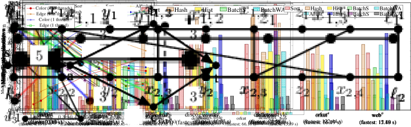
Figure 10: These are the runtimes for butterfly counting per vertex, considering different rankings. We use simple batching as our wedge aggregation method. All times are scaled by the fastest runtime, as indicated in parentheses. Moreover, the time taken to rank each graph is included in the runtimes.

6.2.2 Ranking

Figure 10 shows the runtimes for butterfly counting per vertex for different rankings using the simple batching method. The times are normalized to the time for the fastest ranking for each dataset. Side ordering outperforms the other rankings for itwiki, livejournal, and orkut, while approximate complement degeneracy, approximate degree, and degree orderings outperform side ordering for discogs, enwiki, delicious, and web.

Note that different rankings change the number of wedges that we must process; in particular, we found that complement degeneracy and approximate complement degeneracy minimizes the number of wedges that we process across all of the real-world graphs considered. However, complement degeneracy is not a feasible ordering in practice, since the time for ranking often exceeds the time for the actual counting. Moreover, side ordering often outperforms the other rankings due to better locality, especially if the number of wedges processed by the other rankings does not greatly exceed the number of wedges given by side ordering. We found that the approximate complement degeneracy, degree, and approximate degree orders perform similarly, and these orderings are all efficient to compute.

As such, we devise a metric $f$ that in general determines whether side ordering outperforms other rankings. If we let $w_{s}$ be the number of wedges processed by using side ordering and $w_{r}$ be the number of wedges processed by using another ranking, our metric is $\left.(w_{s}-w_{r})\middle/w_{s}\right.$. If this metric is below $0.1$, then side ordering will outperform or perform just as well as other rankings. Table 3 shows this metric across all of the rankings in ParButterfly. Note that this metric is fairly similar across these other rankings, and is particularly high for web, explaining the significant speedup obtained by using approximate degree ordering over side ordering for web. The $f$ metric can be computed at runtime, before actually ranking the graph, to decide which ordering to use.

6.2.3 Approximate counting

Figure 11 shows runtimes for both colorful sparsification and edge sparsification on orkut, as well as the corresponding single-threaded times. We see that over a variety of probabilities $p$ we achieve self-relative speedups between 4.9–21.4x.

Table 3: These are the fractional values $f=\left.(w_{s}-w_{r})\middle/w_{s}\right.$, where $w_{s}$ is the number of wedges that must be processed using side ordering and $w_{r}$ is the number of wedges that must be processed using the labeled ordering. Note that for itwiki, the number of wedges produced by degree ordering is precisely equal to the number of wedges produced by side ordering.

Dataset	Complement Degeneracy	Approx Complement Degeneracy	Degree	Approx Degree
itwiki	0.021	0.020	0	-0.00033
discogs	0.97	0.97	0.97	0.96
livejournal	0.035	0.033	0.011	-0.019
enwiki	0.47	0.47	0.45	0.46
delicious	0.60	0.60	0.59	0.59
orkut	0.070	0.064	0.042	0.029
web	0.95	0.95	0.95	0.95

Figure 11: These are the runtimes for colorful sparsification and edge sparsification over different probabilities $p$. We considered both the runtimes on 48 cores hyperthreaded and on a single thread. We ran these algorithms on orkut, using simple batch aggregation and side ranking.

Figure 12: These are the parallel runtimes for butterfly vertex peeling with different wedge aggregation methods (these runtimes do not include the time taken to count butterflies). All times are scaled by the fastest parallel time, as indicated in parentheses. Also, note that the runtimes for discogs_style represent single-threaded runtimes; this is because we did not see any parallel speedups for discogs_style, due to the small number of vertices that were peeled.

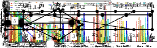
Figure 13: These are the parallel runtimes for butterfly edge peeling with different wedge aggregation methods (these runtimes do not include the time taken to count butterflies). All times are scaled by the fastest parallel time, as indicated in parentheses.

Table 4: These are runtimes in seconds for parallel and single-threaded butterfly peeling from ParButterfly (PB) and serial butterfly peeling from Sariyüce and Pinar [54]. Note that these runtimes do not include the time taken to count butterflies. For the runtimes from ParButterfly, we have noted the aggregation method used; ^∗ refers to simple batching, ^# refers to sorting and ^∘ refers to histogramming.

	Vertex Peeling			Edge Peeling
Dataset	PB $T_{48\text{h}}$	PB $T_{1}$	Sariyüce and Pinar [54] $T_{1}$	PB $T_{48\text{h}}$	PB $T_{1}$	Sariyüce and Pinar [54] $T_{1}$
dblp	$0.91^{\circ}$	$2.40^{\circ}$	2.06	$2.06^{\circ}$	$16.90^{\circ}$	6.93
github	$0.87^{\circ}$	$1.03^{\circ}$	1.15	$5.25^{*}$	$18.00^{*}$	18.82
discogs	$26^{\circ}$	$53.10^{*}$	157.14	$306^{*}$	$2160^{*}$	2149.54
discogs_style	$0.48^{*}$	$0.48^{*}$	14826.16	$2380^{\#}$	$15600^{*}$	16449.56
delicious	$853^{\circ}$	$1900^{*}$	2184.27	—	—	—

6.2.4 Butterfly peeling

Figures 12 and 13 show the runtimes over different wedge aggregation methods for vertex peeling and edge peeling, respectively (the runtimes do not include the time for counting butterflies). We only report times for the datasets for which finished within 5.5 hours. We find that for vertex peeling, aggregation by histogramming largely gives the best runtimes, while for edge peeling, all of our aggregation methods give similar results.

We compare our parallel peeling times to our single-threaded peeling times and serial peeling times from Sariyüce and Pinar’s [54] implementation, which we ran in our environment and which are shown in Table 4. Compared to Sariyüce and Pinar [54], we achieve speedups between 1.3–30696x for vertex peeling and between 3.4–7.0x for edge peeling. Our speedups are highly variable because they depend heavily on the peeling complexities and the number of empty buckets processed. Our largest speedup of 30696x occurs for vertex peeling on discogs_style where we are able to efficiently skip over many empty buckets, while the implementation of Sariyüce and Pinar sequentially iterates over the empty buckets.

Moreover, comparing our parallel peeling times to their corresponding single-threaded times, we achieve speedups between 1.0–10.7x for vertex peeling and between 2.3–10.4x for edge peeling. We did not see self-relative parallel speedups for vertex peeling on discogs_style, because the total number of vertices peeled (383) was too small.

Figure 14: These are the parallel runtimes for butterfly counting per vertex (using the cache optimization), considering different wedge aggregation and butterfly aggregation methods. We consider the ranking that produces the fastest runtime for each graph; ^∗ refers to side ranking, ^◆ refers to degree ranking, and ^∘ refers to approximate degree ranking. All times are scaled by the fastest parallel time, as indicated in parentheses.

6.3 Cache optimization for butterfly counting

We find that using Wang et al.’s [65] cache optimization for total, per-vertex, and per-edge parallel butterfly counting gives speedups of up to 1.7x of our parallel butterfly counting algorithms without the cache optimization, considering the best aggregation and ranking methods for each case. We present the butterfly counting experiments with the cache optimization enabled in this section. The trends are similar to the results without the cache optimization enabled. Note that the cache optimization does not always improve the performance of butterfly counting; for certain graphs, the best butterfly counting time is obtained without using the optimization.

6.4 Butterfly counting

Table 5: These are runtimes in seconds for sequential butterfly counting from ParButterfly (using the cache optimization), as well as runtimes from previous work. Note that PGD [2] is parallel, while the rest of the implementations are serial. Also, for the runtimes from our framework, we have noted the ranking used; ^∗ refers to side ranking, ^# refers to approximate complement degeneracy ranking, ^◆ refers to degree ranking, and ^∘ refers to approximate degree ranking. We have also noted the wedge aggregation and butterfly aggregation methods used for the parallel runtimes; ^⋆ refers to hashing with atomic adds, ^◆ refers to histogramming for both aggregation methods, and ^□ refers to wedge-aware batching. The rest of the parallel runtimes were obtained using simple batching.

	Total Counts					Per-Vertex Counts			Per-Edge Counts
Dataset	PB $T_{48\text{h}}$	PB $T_{1}$	Sanei-Mehri et al. [53] $T_{1}$	PGD [2] $T_{48\text{h}}$	ESCAPE [50] $T_{1}$	PB $T_{48\text{h}}$	PB $T_{1}$	Sariyüce and Pinar [54] $T_{1}$	PB $T_{48\text{h}}$	PB $T_{1}$	Sariyüce and Pinar [54] $T_{1}$
itwiki	$0.10^{*}$	$1.22^{\circ}$	1.63	1798.43	4.97	$0.14^{*}$	$1.46^{*}$	6.06	$0.41^{*\square}$	$4.77^{*}$	19314.87
discogs	$0.81^{\#\blacklozenge}$	$1.20^{\lozenge}$	4.12	234.48	2.08	$0.83^{\circ\star}$	$0.90^{\#}$	96.09	$0.52^{\circ}$	$2.97^{\circ}$	1089.04
livejournal	$3.83^{*}$	$35.12^{*}$	37.80	$>$ 5.5 hrs	139.06	$5.58^{*}$	$38.91^{*}$	158.79	$8.91^{\lozenge}$	$106.07^{*}$	$>$ 5.5 hrs
enwiki	$5.59^{\circ}$	$59.18^{\circ}$	69.10	$>$ 5.5 hrs	151.63	$8.31^{\circ}$	$54.71^{\circ}$	608.53	$11.58^{\circ}$	$152.92^{\circ}$	$>$ 5.5 hrs
delicious	$8.05^{\circ}$	$82.43^{\circ}$	162.00	$>$ 5.5 hrs	286.86	$11.93^{\circ}$	$96.18^{\circ}$	1027.12	$15.98^{\circ}$	$210.70^{\circ}$	$>$ 5.5 hrs
orkut	$22.47^{\#}$	$414.02^{*}$	403.46	$>$ 5.5 hrs	1321.20	$41.57^{\circ}$	$557.10^{*}$	2841.27	$89.52^{\circ}$	$1141.05^{*}$	$>$ 5.5 hrs
web	$8.08^{\circ}$	$61.68^{\circ}$	4340	$>$ 5.5 hrs	172.77	$13.63^{\lozenge}$	$77.82^{\circ}$	$>$ 5.5 hrs	$14.08^{\lozenge}$	$154.35^{\circ}$	$>$ 5.5 hrs

Figures 14, 15, and 16 show the runtimes over different aggregation methods for counting per vertex, per edge, and in total, respectively, for the seven datasets in Figure 1 with sequential counting times exceeding 1 second. The times are normalized to the fastest combination of aggregation and ranking methods for each dataset. Considering different wedge and butterfly aggregation methods, we again find that simple batching and wedge-aware batching give the best runtimes for butterfly counting in general. Of the work-efficient aggregation methods, hashing with atomic adds is often the fastest, particularly for larger graphs due to increased parallelism.

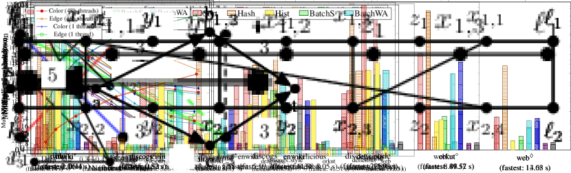
Figure 15: These are the parallel runtimes for butterfly counting per edge (using the cache optimization), considering different wedge aggregation and butterfly aggregation methods. We consider the ranking that produces the fastest runtime for each graph; ^∗ refers to side ranking, ^◆ refers to degree ranking, and ^∘ refers to approximate degree ranking. All times are scaled by the fastest parallel time, as indicated in parentheses.

Figure 16: These are the parallel runtimes for butterfly counting in total (using the cache optimization), considering different wedge aggregation methods (butterfly aggregation does not apply). We consider the ranking that produces the fastest runtime for each graph; ^∗ refers to side ranking, ^# refers to approximate complement degeneracy ranking, and ^∘ refers to approximate degree ranking. All times are scaled by the fastest parallel time, as parentheses.

Also, Figure 5 shows the runtimes for the sequential counting implementations using the cache optimization, as well as runtimes for implementations from previous works, all of which were tested on the same machine. Our configurations achieve parallel speedups of between 5.7–18.0x over the best sequential implementations for large enough graphs. We improve upon PGD [2] by 289.5–5170x.

Figure 17: These are the runtimes for butterfly counting per vertex on livejournal using side ranking and using the cache optimization, over different numbers of threads. The self-relative speedups are between 14.1–37.4x.

Figure 18: These are the runtimes for butterfly counting per edge on livejournal using approximate degree ranking and using the cache optimization, over different numbers of threads. The self-relative speedups are between 9.8–38.9x.

Figures 18 and 18 show our self-relative speedups on livejournal for per-vertex and per-edge counting, respectively, using the cache optimization. Across all rankings, on livejournal, we achieve self-relative speedups between 14.1–37.4x for per-vertex counting and between 9.8–38.9x for per-edge counting.

6.4.1 Ranking

Figure 19 shows the runtimes for butterfly counting per vertex for different rankings using the simple batching method with the cache optimization. The times are normalized to the time for the fastest ranking for each dataset. Side ordering outperforms the other rankings for itwiki and livejournal, while approximate complement degeneracy, approximate degree, and degree orderings outperform side ordering for discogs, enwiki, delicious, orkut, and web.

Figure 19: These are the parallel runtimes for butterfly counting per vertex (using the cache optimization), considering different rankings. We use simple batching as our wedge aggregation method. All times are scaled by the fastest parallel time, as indicated in parentheses. Moreover, the time taken to rank each graph is included in the runtimes.

6.4.2 Approximate counting

Figure 11 shows runtimes with the cache optimization for both colorful sparsification and edge sparsification on orkut, as well as the corresponding single-threaded times. We see that over a variety of probabilities $p$ we achieve self-relative speedups between 5.4–18.9x.

Figure 20: These are the runtimes for colorful sparsification and edge sparsification over different probabilities $p$ (using the cache optimization). We considered both the runtimes on 48 cores hyperthreaded and on a single thread. We ran these algorithms on orkut, using simple batch aggregation and side ranking.

7 Related Work

There have been several sequential algorithms designed for butterfly counting and peeling. Wang et al. [64] propose the first algorithm for butterfly counting over vertices in $\operatorname{O}\bigl{(}\sum_{v\in V}\text{deg}(v)^{2}\bigr{)}$ work, and Sanei-Mehri et al. [53] introduce a practical speedup by choosing the vertex partition with fewer wedges to iterate over. Sanei-Mehri et al. [53] also introduce approximate counting algorithms based on sampling and graph sparsification. Later, Zhu et al. [70] present a sequential algorithm for counting over vertices based on ordering vertices (although they do not specify which order) in $\operatorname{O}\bigl{(}\sum_{v\in V}\text{deg}(v)^{2}\bigr{)}$ work. They extend their algorithm to the external-memory setting and also design sampling algorithms. Chiba and Nishizeki’s [14] original work on counting $4$-cycles in general graphs applies directly to butterfly counting in bipartite graphs and has a better work complexity. Chiba and Nishizeki [14] use a ranking algorithm that counts the total number of $4$-cycles in a graph in $\operatorname{O}\bigl{(}\alpha m\bigr{)}$ work, where $\alpha$ is the arboricity of the graph. While they only give a total count in their work, their algorithm can easily be extended to obtain counts per-vertex and per-edge in the same time complexity. Butterfly counting using degree ordering was also described by Xia [68]. Sariyüce and Pinar [54] introduce algorithms for butterfly counting over edges, which similarly takes $\operatorname{O}\bigl{(}\sum_{v\in V}\text{deg}(v)^{2}\bigr{)}$ work. Zou [71] develop the first algorithm for butterfly peeling per edge, with $\operatorname{O}\bigl{(}m^{2}+m\cdot\text{max-b}_{e}\bigr{)}$ work. Sariyüce and Pinar [54] give algorithms for butterfly peeling over vertices and over edges, which take $\operatorname{O}\bigl{(}\text{max-b}_{v}+\sum_{u\in U}\text{deg}(u)^{2}\bigr{)}$ work and $\operatorname{O}\bigl{(}\text{max-b}_{e}+\sum_{u\in U}\sum_{v_{1},v_{2}\in N(u)}\allowbreak\text{max}(\text{deg}(v_{1}),\text{deg}(v_{2}))\bigr{)}$ work, respectively. Very recently, Wang et al. [66] present a sequential algorithm for butterfly edge peeling that improves over the algorithm by Sariyüce and Pinar [54] in practice, and uses an index that takes $\operatorname{O}\bigl{(}\alpha m\bigr{)}$ space.

In terms of prior work on parallelizing these algorithms, Wang et al. [64] implement a distributed algorithm using MPI that partitions the vertices across processors, and each processor sequentially counts the number of butterflies for vertices in its partition. They also implement a MapReduce algorithm, but show that it is less efficient than their MPI-based algorithm. The largest graph they report parallel times for is the deli graph with 140 million edges and $1.8\times 10^{10}$ butterflies; this is the delicious tag-item graph in KONECT [38]. On this graph, they take 110 seconds on 16 nodes, whereas on the same graph we take 5.17 seconds on 16 cores.

Very recently, and independently of our work, Wang et al. [65] describe an algorithm for butterfly counting using degree ordering, as done in Chiba and Nishizeki [14], and also propose a cache optimization for wedge retrieval. Their parallel algorithm is our parallel algorithm with simple batching for wedge aggregation, except they manually schedule the threads, while we use the Cilk scheduler. They use their algorithm to speed up approximate butterfly counting, and also propose an external-memory variant.

There has been recent work on algorithms for finding subgraphs of size 4 or 5 [31, 22, 50, 2, 17], which can be used for butterfly counting as a special case. Marcus and Shavitt [42] design a sequential algorithm for finding subgraphs of up to size 4. Hocevar and Demsar [31] present a sequential algorithm for counting subgraphs of up to size 5. Pinar et al. [50] also present an algorithm for counting subgraphs of up to size 5 based on degree ordering as done in Chiba and Nishizeki [14]. Elenberg et al. [22] present a distributed algorithm for counting subgraphs of size 4. Ahmed et al. [2] present the PGD shared-memory framework for counting subgraphs of up to size 4. The work of their algorithm for counting $4$-cycles is $\operatorname{O}\bigl{(}\sum_{(u,v)\in E}(\text{deg}(v)+\sum_{u^{\prime}\in N(v)}\text{deg}(u^{\prime}))\bigr{)}$, which is higher than that of our algorithms. Aberger et al. [1] design the EmptyHeaded framework for parallel subgraph finding based on worst-case optimal join algorithms [46]. For butterfly counting, their approach takes quadratic work. We were unable to obtain runtimes for EmptyHeaded because it ran out of memory in our environment. Dave et al. [17] present a parallel method for counting subgraphs of up to size 5 local to each edge. For counting $4$-cycles, their algorithm is the same as PGD, which we compare with. There have also been various methods for approximating subgraph counts via sampling [36, 3, 4, 67, 34, 13, 52, 44]. Finally, there has also been significant work for the past decade on parallel triangle counting algorithms (e.g., [59, 7, 60, 6, 48, 49, 15, 47, 61, 63, 41, 37, 28, 27, 32, 20, 30, 69] and papers from the annual GraphChallenge [26], among many others).

8 Conclusion

We have designed a framework ParButterfly that provides efficient parallel algorithms for butterfly counting (global, per-vertex, and per-edge) and peeling (by vertex and by edge). We have also shown strong theoretical bounds in terms of work and span for these algorithms. The ParButterfly framework is built with modular components that can be combined for practical efficiency. ParButterfly outperforms the best existing parallel butterfly counting implementations, and we outperform the fastest sequential baseline by up to 13.6x for butterfly counting and by up to several orders of magnitude for butterfly peeling.

References

- [1] Christopher R. Aberger, Andrew Lamb, Susan Tu, Andres Nötzli, Kunle Olukotun, and Christopher Ré. EmptyHeaded: A relational engine for graph processing. ACM Trans. Database Syst., 42(4):20:1–20:44, 2017.
- [2] Nesreen K. Ahmed, Jennifer Neville, Ryan A. Rossi, Nick G. Duffield, and Theodore L. Willke. Graphlet decomposition: framework, algorithms, and applications. Knowl. Inf. Syst., 50(3):689–722, 2017.
- [3] Nesreen K. Ahmed, Theodore L. Willke, and Ryan A. Rossi. Estimation of local subgraph counts. In IEEE International Conference on Big Data, pages 586–595, 2016.
- [4] Nesreen K. Ahmed, Theodore L. Willke, and Ryan A. Rossi. Exact and estimation of local edge-centric graphlet counts. In International Workshop on Big Data, Streams and Heterogeneous Source Mining: Algorithms, Systems, Programming Models and Applications, pages 1–17, 2016.
- [5] Sinan G. Aksoy, Tamara G. Kolda, and Ali Pinar. Measuring and modeling bipartite graphs with community structure. J. Complex Networks, 5:581–603, 2017.
- [6] Shaikh Arifuzzaman, Maleq Khan, and Madhav Marathe. PATRIC: A parallel algorithm for counting triangles in massive networks. In ACM Conference on Information and Knowledge Management (CIKM), pages 529–538, 2013.
- [7] A. Azad, A. Buluç, and J. Gilbert. Parallel triangle counting and enumeration using matrix algebra. In IEEE International Parallel and Distributed Processing Symposium Workshop, pages 804–811, 2015.
- [8] Luca Becchetti, Paolo Boldi, Carlos Castillo, and Aristides Gionis. Efficient semi-streaming algorithms for local triangle counting in massive graphs. In ACM SIGKDD International Conference on Knowledge Discovery and Data Mining, pages 16–24, 2008.
- [9] Divya Bhattarai. Towards scalable parallel fibonacci heap implementation. Master’s thesis, St. Cloud State University, 2018.
- [10] Guy E. Blelloch, Phillip B. Gibbons, and Harsha Vardhan Simhadri. Low depth cache-oblivious algorithms. In ACM Symposium on Parallelism in Algorithms and Architectures (SPAA), pages 189–199, 2010.
- [11] Robert D. Blumofe and Charles E. Leiserson. Scheduling multithreaded computations by work stealing. J. ACM, 46(5):720–748, September 1999.
- [12] Stephen P. Borgatti and Martin G. Everett. Network analysis of 2-mode data. Social Networks, 19(3):243 – 269, 1997.
- [13] Marco Bressan, Flavio Chierichetti, Ravi Kumar, Stefano Leucci, and Alessandro Panconesi. Motif counting beyond five nodes. TKDD, 12(4):48:1–48:25, 2018.
- [14] Norishige Chiba and Takao Nishizeki. Arboricity and subgraph listing algorithms. SIAM J. Comput., 14(1):210–223, February 1985.
- [15] Jonathan Cohen. Graph twiddling in a MapReduce world. Computing in Science and Eng., 11(4):29–41, July 2009.
- [16] Thomas H. Cormen, Charles E. Leiserson, Ronald L. Rivest, and Clifford Stein. Introduction to Algorithms (3. ed.). MIT Press, 2009.
- [17] V. S. Dave, N. K. Ahmed, and M. Hasan. PE-CLoG: Counting edge-centric local graphlets. In IEEE International Conference on Big Data, pages 586–595, 2017.
- [18] Inderjit S. Dhillon. Co-clustering documents and words using bipartite spectral graph partitioning. In ACM SIGKDD International Conference on Knowledge Discovery and Data Mining, pages 269–274, 2001.
- [19] Laxman Dhulipala, Guy Blelloch, and Julian Shun. Julienne: A framework for parallel graph algorithms using work-efficient bucketing. In ACM Symposium on Parallelism in Algorithms and Architectures (SPAA), pages 293–304, 2017.
- [20] Laxman Dhulipala, Guy E. Blelloch, and Julian Shun. Theoretically efficient parallel graph algorithms can be fast and scalable. In ACM Symposium on Parallelism in Algorithms and Architectures (SPAA), pages 393–404, 2018.
- [21] James R. Driscoll, Harold N. Gabow, Ruth Shrairman, and Robert E. Tarjan. Relaxed heaps: An alternative to fibonacci heaps with applications to parallel computation. Commun. ACM, 31(11):1343–1354, November 1988.
- [22] Ethan R. Elenberg, Karthikeyan Shanmugam, Michael Borokhovich, and Alexandros G. Dimakis. Distributed estimation of graph 4-profiles. In International Conference on World Wide Web (WWW), pages 483–493, 2016.
- [23] Michael L. Fredman and Robert Endre Tarjan. Fibonacci heaps and their uses in improved network optimization algorithms. J. ACM, 34(3):596–615, July 1987.
- [24] David Gibson, Ravi Kumar, and Andrew Tomkins. Discovering large dense subgraphs in massive graphs. In Proceedings of the 31st International Conference on Very Large Data Bases, pages 721–732. VLDB Endowment, 2005.
- [25] J. Gil, Y. Matias, and U. Vishkin. Towards a theory of nearly constant time parallel algorithms. In IEEE Symposium on Foundations of Computer Science (FOCS), pages 698–710, 1991.
- [26] GraphChallenge. http://graphchallenge.mit.edu/.
- [27] Oded Green, Luis M. Munguia, and David A. Bader. Load balanced clustering coefficients. In Workshop on Parallel Programming for Analytics Applications, pages 3–10, 2014.
- [28] Oded Green, Pavan Yalamanchili, and Luis M. Munguia. Fast triangle counting on the GPU. In Workshop on Irregular Applications: Architectures and Algorithms, pages 1–8, 2015.
- [29] Yan Gu, Julian Shun, Yihan Sun, and Guy E. Blelloch. A top-down parallel semisort. In ACM Symposium on Parallelism in Algorithms and Architectures (SPAA), pages 24–34, 2015.
- [30] Shuo Han, Lei Zou, and Jeffrey Xu Yu. Speeding up set intersections in graph algorithms using simd instructions. In ACM SIGMOD International Conference on Management of Data, pages 1587–1602, 2018.
- [31] Tomaz Hocevar and Janez Demsar. A combinatorial approach to graphlet counting. Bioinformatics, pages 559–65, 2014.
- [32] Yang Hu, Hang Liu, and H. Howie Huang. TriCore: Parallel triangle counting on gpus. In International Conference for High Performance Computing, Networking, Storage, and Analysis (SC), pages 14:1–14:12, 2018.
- [33] Qin Huang and W. E. Weihl. An evaluation of concurrent priority queue algorithms. In IEEE Symposium on Parallel and Distributed Processing, pages 518–525, 1991.
- [34] Shweta Jain and C. Seshadhri. A fast and provable method for estimating clique counts using Turán’s theorem. In International Conference on World Wide Web (WWW), pages 441–449, 2017.
- [35] J. Jaja. Introduction to Parallel Algorithms. Addison-Wesley Professional, 1992.
- [36] Madhav Jha, C. Seshadhri, and Ali Pinar. Path sampling: A fast and provable method for estimating 4-vertex subgraph counts. In International Conference on World Wide Web (WWW), pages 495–505, 2015.
- [37] Tamara G. Kolda, Ali Pinar, Todd Plantenga, C. Seshadhri, and Christine Task. Counting triangles in massive graphs with MapReduce. SIAM Journal on Scientific Computing, 36(5):S48–S77, 2014.
- [38] Jérôme Kunegis. KONECT: the Koblenz network collection. pages 1343–1350, 05 2013.
- [39] Matthieu Latapy, Clémence Magnien, and Nathalie Del Vecchio. Basic notions for the analysis of large two-mode networks. Social Networks, 30(1):31 – 48, 2008.
- [40] Charles E. Leiserson. The Cilk++ concurrency platform. The Journal of Supercomputing, 51(3), 2010.
- [41] D. Makkar, D. A. Bader, and O. Green. Exact and parallel triangle counting in dynamic graphs. In IEEE International Conference on High Performance Computing (HiPC), pages 2–12, 2017.
- [42] D. Marcus and Y. Shavitt. Efficient counting of network motifs. In IEEE International Conference on Distributed Computing Systems Workshops, pages 92–98, 2010.
- [43] David W. Matula and Leland L. Beck. Smallest-last ordering and clustering and graph coloring algorithms. J. ACM, 30(3):417–427, July 1983.
- [44] D. Mawhirter, B. Wu, D. Mehta, and C. Ai. ApproxG: Fast approximate parallel graphlet counting through accuracy control. In IEEE/ACM International Symposium on Cluster, Cloud and Grid Computing (CCGRID), pages 533–542, 2018.
- [45] M. E. J. Newman. The structure and function of complex networks. SIAM Review, 45:167–256, 2003.
- [46] Hung Q. Ngo, Ely Porat, Christopher Ré, and Atri Rudra. Worst-case optimal join algorithms. J. ACM, 65(3):16:1–16:40, March 2018.
- [47] Rasmus Pagh and Charalampos E. Tsourakakis. Colorful triangle counting and a MapReduce implementation. Inf. Process. Lett., 112(7):277–281, March 2012.
- [48] Ha-Myung Park and Chin-Wan Chung. An efficient MapReduce algorithm for counting triangles in a very large graph. In ACM Conference on Information and Knowledge Management (CIKM), pages 539–548, 2013.
- [49] Ha-Myung Park, Francesco Silvestri, U Kang, and Rasmus Pagh. MapReduce triangle enumeration with guarantees. In ACM Conference on Information and Knowledge Management (CIKM), pages 1739–1748, 2014.
- [50] Ali Pinar, C. Seshadhri, and Vaidyanathan Vishal. ESCAPE: Efficiently counting all 5-vertex subgraphs. In International Conference on World Wide Web (WWW), pages 1431–1440, 2017.
- [51] S. Rajasekaran and J. H. Reif. Optimal and sublogarithmic time randomized parallel sorting algorithms. SIAM J. Comput., 18(3):594–607, June 1989.
- [52] Ryan A. Rossi, Rong Zhou, and Nesreen K. Ahmed. Estimation of graphlet counts in massive networks. IEEE Trans. Neural Netw. Learning Syst., 30(1):44–57, 2019.
- [53] Seyed-Vahid Sanei-Mehri, Ahmet Erdem Sariyuce, and Srikanta Tirthapura. Butterfly counting in bipartite networks. In ACM SIGKDD International Conference on Knowledge Discovery and Data Mining, pages 2150–2159, 2018.
- [54] Ahmet Erdem Sariyüce and Ali Pinar. Peeling bipartite networks for dense subgraph discovery. In ACM International Conference on Web Search and Data Mining (WSDM), pages 504–512, 2018.
- [55] Stephen B. Seidman. Network structure and minimum degree. Social Networks, 5(3):269 – 287, 1983.
- [56] Jessica Shi and Julian Shun. Parallel algorithms for butterfly computations. In SIAM Symposium on Algorithmic Principles of Computer Systems, pages 16–30, 2020.
- [57] Julian Shun and Guy E. Blelloch. Phase-concurrent hash tables for determinism. In ACM Symposium on Parallelism in Algorithms and Architectures (SPAA), pages 96–107, 2014.
- [58] Julian Shun, Guy E. Blelloch, Jeremy T. Fineman, Phillip B. Gibbons, Aapo Kyrola, Harsha Vardhan Simhadri, and Kanat Tangwongsan. Brief announcement: The Problem Based Benchmark Suite. In ACM Symposium on Parallelism in Algorithms and Architectures (SPAA), pages 68–70, 2012.
- [59] Julian Shun and Kanat Tangwongsan. Multicore triangle computations without tuning. In IEEE International Conference on Data Engineering (ICDE), pages 149–160, 2015.
- [60] Siddharth Suri and Sergei Vassilvitskii. Counting triangles and the curse of the last reducer. In International World Wide Web Conference (WWW), pages 607–614, 2011.
- [61] Kanat Tangwongsan, A. Pavan, and Srikanta Tirthapura. Parallel triangle counting in massive streaming graphs. In ACM Conference on Information and Knowledge Management (CIKM), pages 781–786, 2013.
- [62] Charalampos E. Tsourakakis, Petros Drineas, Eirinaios Michelakis, Ioannis Koutis, and Christos Faloutsos. Spectral counting of triangles via element-wise sparsification and triangle-based link recommendation. Social Network Analysis and Mining, 1(2):75–81, Apr 2011.
- [63] Charalampos E. Tsourakakis, U. Kang, Gary L. Miller, and Christos Faloutsos. DOULION: Counting triangles in massive graphs with a coin. In ACM SIGKDD Conference on Knowledge Discovery and Data Mining, pages 837–846, 2009.
- [64] Jia Wang, Ada Wai-Chee Fu, and James Cheng. Rectangle counting in large bipartite graphs. In IEEE International Congress on Big Data, pages 17–24, 2014.
- [65] Kai Wang, Xuemin Lin, Lu Qin, Wenjie Zhang, and Ying Zhang. Vertex priority based butterfly counting for large-scale bipartite networks. PVLDB, 12(10), June 2019.
- [66] Kai Wang, Xuemin Lin, Lu Qin, Wenjie Zhang, and Ying Zhang. Efficient bitruss decomposition for large-scale bipartite graphs. In IEEE International Conference on Data Engineering (ICDE), 2020.
- [67] P. Wang, J. Zhao, X. Zhang, Z. Li, J. Cheng, J. C. S. Lui, D. Towsley, J. Tao, and X. Guan. MOSS-5: A fast method of approximating counts of 5-node graphlets in large graphs. IEEE Transactions on Knowledge and Data Engineering, 30(1):73–86, Jan 2018.
- [68] Xiangzhou Xia. Efficient and scalable listing of four-vertex subgraphs. Master’s thesis, Texas A&M University, 2016.
- [69] Y. Zhang, H. Jiang, F. Wang, Y. Hua, D. Feng, and X. Xu. LiteTE: Lightweight, communication-efficient distributed-memory triangle enumerating. IEEE Access, 7:26294–26306, 2019.
- [70] R. Zhu, Z. Zou, and J. Li. Fast rectangle counting on massive networks. In IEEE International Conference on Data Mining (ICDM), pages 847–856, 2018.
- [71] Zhaonian Zou. Bitruss decomposition of bipartite graphs. In Database Systems for Advanced Applications, pages 218–233, 2016.