Real-time evolution and quantized charge pumping in magnetic Weyl semimetals

Abstract

Real-time evolution and charge pumping in magnetic Weyl semimetals are studied by solving the time-dependent Schrödinger equations. In the adiabatic limit of the real-time evolution, we show that the total pumped charge is quantized in the magnetic Weyl semimetals as in the quantum Hall system although the Weyl semimetal has no bulk gap. We examine how the disorder affects the charge pumping. As a result, we show that the quantized pumped charge is robust against the small disorder and find that the pumped charge increases in the intermediate disorder region. We also examine the doping effects on the charge pumping and show that the remnant of the quantized pumped charge at zero doping can be detected. Our results show that the real-time evolution is a useful technique for detecting the topological properties of the systems with no bulk gap and/or disorders.

I Introduction

Immediately after the discovery of the integer quantum Hall effects Klitzing et al. (1980), Laughlin presented the simple and important gedanken experiment for explaining the quantized Hall conductivity Laughlin (1981). In the Laughlin’s gedanken experiment, by adiabatically introducing the magnetic flux $\Phi$ from 0 to $\Phi=\Phi_{0}=e/h$ into the quantum Hall system on a cylinder, the electrons move from one edge to opposite side of edge as schematically shown in Fig. 1. Due to the invariance of the wave functions under the gauge transformation by the flux $\Phi$, it is shown that the total pumped charge should be quantized when $\Phi=\Phi_{0}$.

In a similar way, Thouless argued the charge pumping in the one-dimensional systems with the slow time-dependent periodic potentials Thouless (1983). By solving the time-dependent Schrödinger equations, Thouless shows that the pumped charge is quantized and it is related with the topological invariant. The charge pumping caused by introducing the external flux is called the Thouless pumping and the Laughlin’s argument can be regarded as the adiabatic limit of the Thouless pumping. Although the realization of the Thouless pumping in experiment is difficult because introducing the magnetic flux or adiabatically controlling the periodic potential are difficult, recent experiments show that the Thouless pumping can be realized in the ultra cold atoms Nakajima et al. (2016); Lohse et al. (2016).

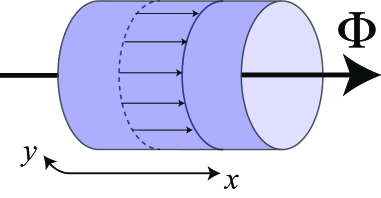
Figure 1: (color online) Schematic picture for the Laughlin’s gedanken experiment in the quantum Hall system. By introducing flux $\Phi$ (equivalently introducing electric field in $y$ direction), charge pumping occurs in $x$ direction.

In a theoretical point of view, the Thouless pumping is a useful theoretical technique for detecting the topological invariant. In the previous studies, the Thouless pumping in the quantum Hall system is numerically studied and it is shown that the charge pumping continuously occurs from $t=0$ ($t$ represents time) and it reaches the quantized value at $t=T$ ($T$ is the time interval during which the magnetization increases by $\Phi_{0}$) in the adiabatic limit Maruyama and Hatsugai (2009); Hatsugai and Fukui (2016). In the quantum Hall systems, the total charge pumping is expressed by the topological invariant as follows Thouless et al. (1982); Kohmoto (1985):

$$\Delta N(t=T)=N_{\rm L}(t=T)-N_{\rm R}(t=T)=2\times\mathcal{C},$$ (1)

where $N_{\rm L}(t)$ ($N_{\rm R}(t)$) denotes the number of electrons distributed in left side (right side) of the system and $\mathcal{C}$ is the topological invariant called the Chern number that takes integers ($\mathcal{C}=0,\pm 1,\pm 2,\cdots$).

In the conventional ways for calculating the topological invariants, it is necessary to define the Bloch wave functions Ryu et al. (2010). Although such definitions are useful for non-interacting systems with translational invariance, they are not directly used for non-periodic systems such as the disordered systems. In the Thouless pumping, by solving the time-dependent Schrödinger equations, it is easy to calculate the topological invariant even for disordered systems through the quantized charge pumping. We note that Thouless pumping may be useful for detecting the topological invariant in the correlated electron systems Nakagawa et al. (2018).

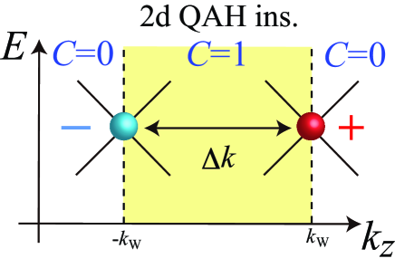
Figure 2: (color online) Schematic picture of the Weyl points in the momentum space. The positions of the Weyl points are denoted by $\pm k_{\rm W}$. Signs of monopole charges Hirayama et al. (2015) at the Weyl points are represented by $+$ and $-$. Inside the Weyl point ($-k_{\rm W}\leq k_{z}\leq k_{\rm W}$), the Chern number is non trivial ($\mathcal{C}=1$) while it is trivial outside the Weyl points ($\mathcal{C}=0$). The Hall conductivity in the Weyl semimetal is given by $\sigma_{xy}=\frac{e^{2}}{h}\frac{\Delta k}{2\pi}$.

In this paper, by using the real-time evolution, we apply the Thouless pumping to the Weyl semimetals where the quantized charge pumping also occurs Shindou and Nagaosa (2001); Murakami (2007); Wan et al. (2011); Burkov and Balents (2011); Burkov (2018). We note that, Weyl semimetals have been recently found in inversion symmetry broken systems such as TaAs Xu et al. (2015); Lv et al. (2015a, b); Yang et al. (2015) and time-reversal symmetry broken systems (magnetic Weyl semimetals) such as Mn₃Sn Kuroda et al. (2017); Ito and Nomura (2017), Heusller alloys Wang et al. (2016); Chang et al. (2016), Co₃Sn₂S₂ Liu et al. (2018); Xu et al. (2018); Wang et al. (2018); Ozawa and Nomura , and Sr_1-yMn_1-zSb₂ Liu et al. (2017). Because the magnetic Weyl semimetals can be constructed by stacking the two-dimensional quantum anomalous Hall (QAH) systems (see Fig.2), it is shown that the Hall conductivity is quantized as follows:

$$\sigma_{xy} =\frac{e^{2}}{h}\frac{\Delta k}{2\pi},$$ (2)

where $\Delta k$ is the distance between two Weyl points. By performing the Thouless pumping in the Weyl semimetal, it is expected that the charge pumping is also quantized as follows:

$$\Delta N =2\Delta k\times\frac{L_{z}}{2\pi},$$ (3)

where $L_{z}$ is the length of the system in $z$ direction. In the Weyl semimetals, however, the charge gap is zero and it is non-trivial whether the Thouless pumping gives the quantized charge pumping for gapless systems or not. In this work, we show that the quantized charge pumping occurs in the adiabatic limit. This result indicates that the Thouless pumping is useful even when the bulk charge gap is absent.

We also examine the effects of the disorder on the Thouless pumping and find that the charge pumping is robust against the small disorder and it increases in the intermediate disorder region. These behaviors are consistent with the previous studies Chen et al. (2015); Shapourian and Hughes (2016); Takane (2016). This indicates that the Thouless pumping also works well for disordered systems.

This paper is organized as follows: In Sec.2.A, we introduce model Hamiltonians for describing the Weyl semimetal and explain the algorithms for solving the time-dependent Schrödinger equation in Sec.2.B. Although the algorithms are explained in the literature Suzuki (1990, 1993, 1994); Nakanishi et al. (1997), to make our paper self contained, we detail how to efficiently solve the time-dependent Schrödinger equations. In Section 3.A, we show the results of the Thouless pumping for clean limit and at zero doping. Then, we examine the disorder effects in Sec. 3.B. We also examine the doping effects in Sec.3.C and show that the Thouless pumping occurs for the finite doping case, i.e., remnant of the quantization can be detected. Finally, Section 4 is devoted to the summary.

II Model and Method

II.1 Lattice Model for Weyl semimetals

The Hamiltonian used in this study is given by

$$H_{\rm W}=\sum_{\nu=x,y,z}H_{\nu}+H_{\rm diag},$$ (4)

$$H_{\nu}=\sum_{j}h_{\nu,j},$$ (5)

$${h_{\nu,j}=c_{j+\boldsymbol{e}_{\nu}}^{\dagger}T_{\nu}c_{j}+{\rm H.c.}},$$ (6)

$$H_{\rm diag}=(2{t_{\rm hop}}-m)\sum_{j}c_{j}^{\dagger}\sigma_{z}c_{j}+\sum_{j}\epsilon_{j}c_{j}^{\dagger}\sigma_{0}c_{j},$$ (7)

$$\epsilon_{j}\in[-W/2,W/2].$$ (8)

where $c_{j}^{\dagger}$ ($c_{j}$) represents the two-component fermion creation (annihilation) operator defined on a site $j$ on the three dimensional cubic lattice spanned by three orthogonal unit vectors $\boldsymbol{e}_{\nu=x,y,z}$. The matrices $T_{\nu}$ are defined as

$$T_{x} ={t_{\rm hop}}(-\sigma_{z}+{\rm i}\sigma_{x})/2,$$ (9)

$$T_{y} ={t_{\rm hop}}(-\sigma_{z}+{\rm i}\sigma_{y})/2,$$ (10)

$$T_{z} =-{t_{\rm hop}}\sigma_{z}/2,$$ (11)

where

$$\sigma_{x}=\begin{pmatrix}0&~{}1\\ 1&~{}0\\ \end{pmatrix},\sigma_{y}=\begin{pmatrix}0&~{}-{\rm i}\\ {\rm i}&~{}0\\ \end{pmatrix},\sigma_{z}=\begin{pmatrix}1&~{}0\\ 0&~{}-1\\ \end{pmatrix}.$$ (12)

Throughout this paper, we take the amplitude of the hopping transfer $t_{\rm hop}=1$ as a unit of the energy scale.

The band structure of the Hamiltonian is given by

$${E_{\rm W}}={\pm}[(\sin{k_{x}})^{2}+(\sin{k_{y}})^{2}$$

$$+(2-m-\cos{k_{x}}-\cos{k_{y}}-\cos{k_{z}})^{2}]^{1/2}$$ (13)

From this band structure, we can show that the Weyl points are located at $(0,0,k_{\rm W}=\pm\cos^{-1}(-m))$ for $|m|<1$. Around the Weyl points, the dispersions are given as

$${E_{\rm W}}\sim\pm(k_{x}^{2}+k_{y}^{2}+\tilde{k}_{z}^{2})^{1/2},$$ (14)

where $\tilde{k}_{z}=\sqrt{1-m^{2}}(k_{z}-\cos^{-1}(-m))$. We note that the Weyl semimetal is constructed by stacking the two dimensional QAH insulators. As shown in Fig. 2, the Chern number becomes nontrivial inside between the two Weyl points and it becomes trivial outside the Weyl points. Thus, the quantized Hall conductivity is proportional to $\Delta k=2k_{\rm W}$.

To perform the Thouless pumping, we introduce the time-dependent vector potentials as follows:

$$T_{y}(t)=e^{{\rm i}A_{y}(t)}\times T_{y},$$ (15)

$$A_{y}(t)=\frac{2\pi t}{L_{y}T}.$$ (16)

By introducing $A_{y}(t)$ in $y$ direction, the charge pumping in $x$ directions occurs if the Hall conductivity is finite.

II.2 Method for solving the time-dependent Schrödinger equations

To perform the Thouless pumping, we explicitly solve the time-dependent Schrödinger equation defined as

$${\rm i}\frac{\partial\ket{\phi(t)}}{\partial t}=H_{\rm W}\ket{\phi(t)}.$$ (17)

Here, $\ket{\phi(t)}$ is a single Slater determinant given by

$$\ket{\phi(t)}=\prod_{n=1}^{N_{\rm e}}\Big{(}\sum_{i=0}^{N_{\rm s}-1}\Phi_{ni}(t){c}_{i}^{\dagger}\Big{)}\ket{0},$$ (18)

where $N_{\rm e}$ is number of particles, $N_{\rm s}$ is number of sites, and $\Phi_{ni}(t)$ denotes the coefficient of the Slater determinant. By discretizing the time and multiplying the time-evolution operator $U(t+\Delta t,t)$ to the wave functions at each discretized time step, we can solve the time-dependent Schrödinger equations as follows:

$$\ket{\phi(t+\Delta t)} =U(t+\Delta t,t)\ket{\phi(t)},$$ (19)

$$U(t+\Delta t,t) =\mathcal{T}\Big{(}\exp{\Big{[}-{\rm i}\int_{t}^{t+\Delta t}H_{W}(s){\rm d}s]}\Big{)},$$ (20)

where $\mathcal{T}$ it the time ordering operator.

One simple way to solve the time-dependent Schrödinger equation is given by

$$|\phi(t+\Delta t)\rangle\sim\exp{(-{\rm i}\Delta tH_{W}(t))}|\phi(t)\rangle.$$ (21)

Here, we approximate $U(t+\Delta,t)$ as $\exp{(-{\rm i}\Delta tH_{W}(t))}$ and we denote the coefficients of the Hamiltonian as $\tilde{H}_{W}$, i.e., $H_{W}(t)={c}^{\dagger}\tilde{H}_{W}(t){c}$. By diagonalizing $\tilde{H}_{W}(t)$ at each time step, we obtain the solutions as follows:

$${e^{-{\rm i}\Delta t\cdot{c}^{\dagger}\tilde{H}_{W}(t){c}}\ket{\phi(t)}} =\prod_{n=1}^{N_{\rm e}}\Big{(}\sum_{i=0}^{N_{\rm s}-1}{\Phi}_{ni}(t+\Delta t){c}_{i}^{\dagger}\Big{)}\ket{0},$$ (22)

$${\Phi}_{ni}(t+\Delta t) ={\sum_{\alpha j}{\Phi_{nj}(t)}e^{-{\rm i}\Delta t\lambda_{\alpha}}(V^{\dagger})_{\alpha j}V_{i\alpha}},$$ (23)

$$V^{\dagger}{\tilde{H}_{W}(t)}V ={\rm diag}(\lambda_{0},\lambda_{1},\dots,{\lambda_{2N_{\rm s}-1}}).$$ (24)

Because this method requires the diagonalization of the Hamiltonian at each step, the computational costs are large. To reduce the costs, we decompose the time-evolution operator by using the Suzuki-Trotter decomposition Suzuki (1990, 1993, 1994). In this method, because the diagonalization of the full Hamiltonian is necessary only for preparing the initial wave functions, computational cost is drastically reduced.

From here, we explain outline of the method. Since the cubic lattice is bipartite, we decompose the nearest-neighbor-hopping terms in the Hamiltonian into two parts as follows:

$${H}_{\nu} ={H}_{\nu,e}+{H}_{\nu,o},$$ (25)

$${H}_{\nu,e} ={h}_{\nu,0}+{h}_{\nu,2}+\cdots,$$ (26)

$${H}_{\nu,o} ={h}_{\nu,1}+{h}_{\nu,3}+\cdots,$$ (27)

where $h_{\nu,2n~{}(2n+1)}$ contains hopping terms between sites on $\nu=2n~{}(2n+1)$ and those on $\nu=2n+1~{}(2n+2)$ for $\nu=x,y,z$. We note that each component of the Hamiltonian can be described as

$$h_{\nu,i}=\begin{pmatrix}{c}_{i}^{\dagger}&~{}{c}_{i+{\boldsymbol{e}_{\nu}}}^{\dagger}\end{pmatrix}K_{\nu}\begin{pmatrix}{c}_{i}\\ {c}_{i+{\boldsymbol{e}_{\nu}}}\end{pmatrix}.$$ (28)

For example, $K_{x}$ is given by

$$K_{x}=\frac{1}{2}\begin{pmatrix}0&~{}0&~{}-1&~{}-{\rm i}\\ 0&~{}0&~{}-{\rm i}&~{}1\\ -1&~{}{\rm i}&~{}0&~{}0\\ {\rm i}&~{}1&~{}0&~{}0\\ \end{pmatrix}.$$ (29)

Because $h_{\nu,2j}$ is commutable each other ($h_{\nu,2j+1}$ is also commutable each other), it is easy to decompose $e^{{H}_{\nu,e}}$ and $e^{{H}_{\nu,o}}$ as follows:

$$e^{{H}_{\nu,e}} =e^{{h}_{\nu,0}}\times e^{{h}_{\nu,2}}\times\cdots,$$ (30)

$$e^{{H}_{\nu,o}} =e^{{h}_{\nu,1}}\times e^{{h}_{\nu,3}}\times\cdots.$$ (31)

From this relation, by just diagonalizing ${h}_{\nu,i}$ whose matrix size is $4\times 4$, we can perform the real-time evolutions.

Because $H_{\nu,e}$ and $H_{\nu,o}$ are not commutable, we use the fourth-order Suzuki-Trotter decomposition Suzuki (1990), whose general form is by

$$e^{\eta({A}_{1}+\dots+{A}_{q})}=S(\eta p)S(\eta(1-2p))S(\eta p)+O(\eta^{5}),$$ (32)

$$S(\eta)=e^{\eta{A}_{1}/2}e^{\eta{A}_{2}/2}\cdots e^{\eta{A}_{q-1}/2}e^{\eta{A}_{q}}$$

$$\times e^{\eta{A}_{q-1}/2}\cdots e^{\eta{A}_{1}/2},$$ (33)

$$p=(2-2^{1/3})^{-1},$$ (34)

where $\eta$ is c-number and $A_{q}$ denotes the matrix. By using the formula, we can decompose $e^{\eta H_{\rm W}}$ as follows:

$$e^{\eta{H}_{\rm W}} =S(\eta p)S(\eta(1-2p))S(\eta p),$$ (35)

$$S(\eta) =S_{0}(\eta)e^{\eta{H}_{\rm diag}}S_{1}(\eta),$$ (36)

$$S_{0}(\eta) =e^{\eta{H}_{x,e}/2}e^{\eta{H}_{x,o}/2}e^{\eta{H}_{y,e}/2}e^{\eta{H}_{y,o}/2}$$

$$\times e^{\eta{H}_{z,e}/2}e^{\eta{H}_{i}n{z,o}/2}$$

$$S_{1}(\eta) =e^{\eta{H}_{z,o}/2}e^{\eta{H}_{z,e}/2}e^{\eta{H}_{y,o}/2}e^{\eta{H}_{y,e}/2}$$

$$\times e^{\eta{H}_{x,o}/2}e^{\eta{H}_{x,e}/2}.$$ (37)

If the Hamiltonian is not time-dependent one, this formula has fourth-order precision. For the time-dependent Hamiltonian, the time-evolution operator is defined by using the super operator $\tilde{\mathcal{T}}$ as follows Suzuki (1993, 1994):

$$U(t+\Delta t,t) =\exp{\Big{[}\Delta t(-{\rm i}H(t)+\tilde{\mathcal{T})}\Big{]}},$$ (38)

$$F(t)e^{\Delta t\tilde{\mathcal{T}}}G(t) =F(t+\Delta t)G(t).$$ (39)

Here, $F$ and $G$ are arbitrary functions. We note that the super operator $\tilde{\mathcal{T}}$ only acts on the operators on its left. By using this formula, we decompose $U$ as follows:

$$U(t+\Delta t,t)=S(-{\rm i}\Delta tp,t+(1-p/2)\Delta t)$$

$$\times S(-{\rm i}\Delta t(1-2p),t+p\Delta t/2)$$

$$\times S(-{\rm i}\Delta tp,t+p\Delta t/2)+O(\Delta t^{5}),$$ (40)

where time-dependent $S$ is defined as

$$S(\eta,t) =S_{0}(\eta,t)e^{\eta{H}_{\rm diag}}S_{1}(\eta,t),$$ (41)

$$S_{0}(\eta,t) =e^{\eta{H}_{x,e}/2}e^{\eta{H}_{x,o}/2}e^{\eta{H}_{y,e}(t)/2}$$

$$\times e^{\eta{H}_{y,o}(t)/2}e^{\eta{H}_{z,e}/2}e^{\eta{H}_{z,o}/2}$$

$$S_{1}(\eta,t) =e^{\eta{H}_{z,o}/2}e^{\eta{H}_{z,e}/2}e^{\eta{H}_{y,o}(t)/2}$$

$$\times e^{\eta{H}_{y,e}(t)/2}e^{\eta{H}_{x,o}/2}e^{\eta{H}_{x,e}/2}.$$ (42)

We note that super operator $\tilde{\mathcal{T}}$ operates all the left side operators. By using Eq. (40), we perform the real-time evolution.

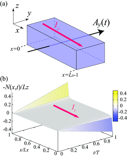
Figure 3: (color online)  (a) Schematic illustration of the geometry used in this study. We take open boundary condition in $x$ direction and the periodic boundary conditions in $y$ and $z$ direction. Employed geometry is given by $L=L_{x}=2L_{y}=2L_{z}$. We introduce the $A_{y}(t)$ in $y$ direction and charge pumping occurs in $x$ direction. (b) Time-dependence of the charge distribution $N(x,t)$ in $x$ direction. We take $m=0$, $T=20$, $W=0$, and $L=44$. The charge pumping occurs around the edges in $x$ direction by introducing $A_{y}(t)$.

III Results

III.1 Thouless pumping in the Weyl semimetals

In Fig. 3(a), we show a setup of Thouless pumping for the Weyl semimetal. The system size is given by $N_{s}=L_{x}\times L_{y}\times L_{z}$ and we employ the rectangle geometry given by $L=L_{x}=2L_{y}=2L_{z}$. In $x$ ($y$ and $z$) direction, we employ the open (periodic) boundary condition. By applying the vector potentials in $y$ direction (Eq. (16)), it is expected that the quantized charge pumping in $x$ direction occurs. We take $\Delta t=0.02$ and $m=0$ in this paper.

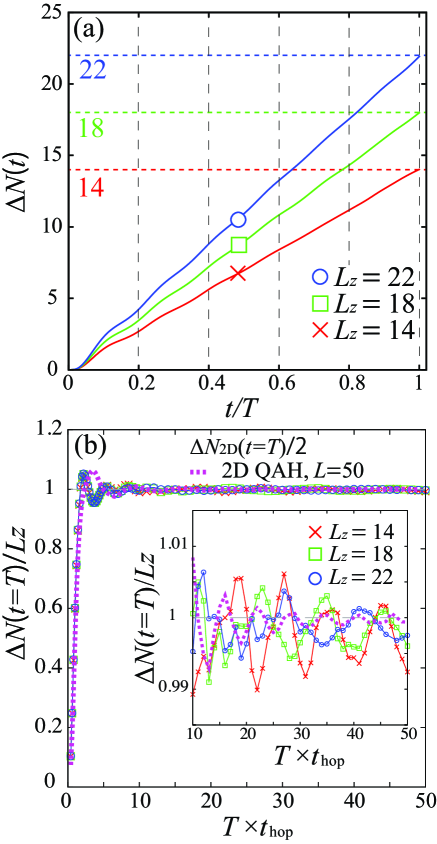
Figure 4: (color online) (a)System size dependence of the charge pumping as a function of time. We take $T=20$, $W=0$ and $m=0$. The charge pumping $t=T$ is quantized as $\Delta N(t=T)=2\Delta k\frac{L_{z}}{2\pi}$, which is proportional to $L_{z}$. (b)  $T$ dependence of the charge pumping. For small $T$, because the introducing $A_{y}(t)$ is not adiabatic, the charge pumping is not quantized. For comparison, we also show $T$ dependence of the charge pumping for the two-dimensional QAH insulator $N_{\rm 2D}(t=T)$, where the bulk gap exists. Details of the two-dimensional QAH insulator are shown in Appendix. For $T\geq 10$, the charge pumping is nearly quantized for both systems except for small oscillations. In the inset, we show enlarged figure for $T\geq 10$. In contrast to the gapped system (see the inset of Fig.9 (b)), for the Weyl semimetal, we find that the small but finite oscillations remains even for larger $T$. This remaining oscillations may originate from the gapless nature of the Weyl semimetal.

In this setup, we perform the Thouless pumping, i.e., solving the time dependent Schrödinger equations and obtain $|\phi(t)\rangle$. From $|\phi(t)\rangle$, we calculate the time-dependent charge distribution in $x$ direction, which is defined as

$$N(x,t)= \sum_{y,z}\Big{[}\bra{\phi(t)}c_{x,y,z}^{\dagger}c_{x,y,z}\ket{\phi(t)}$$

$$-\bra{\phi(0)}c_{x,y,z}^{\dagger}c_{x,y,z}\ket{\phi(0)}\Big{]}.$$ (43)

As shown in Fig. 3(b), by introducing the vector potentials in $y$ direction, the charge pumping in $x$ direction occurs, i.e., $N(x,t)$ becomes positive around $x=0$ while it becomes negative around $x=L_{x}-1$. This result shows that the pumped charge is mainly induced at the edges in the clean limit.

At $t=T$, the total pumped charge is expected to be quantized for sufficiently large $T$. Total pumped charge is defined as

$$\Delta N(t)=\sum_{0\leq x<L_{x}/2}N(x,t)-\sum_{L_{x}/2\leq x<L_{x}}N(x,t)$$ (44)

We show $\Delta N(t)$ for several different system sizes in Fig. 4 (a). We find that $\Delta N(t)$ monotonically increase as a function of $t$ and it nearly becomes $L_{z}$ at $t=T$. This is consistent with the topological properties of the Weyl semimetals, i.e., the Hall conductivity is quantized as $\sigma_{xy}=(e^{2}/2\pi h)\times\Delta k$ and the corresponding charge pumping is given by $\Delta N=(\Delta k/\pi)\times L_{z}$. This result indicates that the Thouless pumping works well even when the systems have no bulk gaps.

To examine when the Thouless pumping can be regarded as the adiabatic process, we calculate unit time ($T$) dependence of the charge pumping. In Fig. 4 (b), we show $T$ dependence of $\Delta N(t=T)$ for several different system sizes. For small $T$ ($T<1$), speed of introducing $A_{y}(t)$ is too fast to change the electronic states in the Weyl semimetals. Thus, for $T<1$, the Thouless pumping is non-adiabatic and the pumped charge is not quantized. By increasing $T$, for $T\geq 10$, the pumped charge is quantized except for small oscillations. This result indicates that the Thouless pumping can be regarded as the adiabatic process for $T\geq 10$. Thus, we take $T=20$ in the most remaining part of this paper. We note that the typical time scale does not significantly change for weak disorder region but it becomes large for strong disorder region. Nevertheless, we note that the charge pumping at $T=20$ can be regarded as the adiabatic pumping in the relevant disorder region.

We note that the Laughlin’s argument or the Thouless’s argument requires the existence of the bulk charge gap for the quantized charge pumping. The Weyl semimetal has no bulk charge gap and it is unclear whether the Thouless pumping works well or not. By comparing with $T$ dependence in the two-dimensional QAH insulator as shown in Fig. 4 (b), we find that $T$ dependence of the pumped charge for the Weyl semimetal is basically the same as that of the QAH insulator. This result clearly shows that the Thouless pumping works well for detecting the topological invariant even when the systems have no bulk gap.

III.2 Effects of disorders

We examine how the disorder affects the charge pumping in the Weyl semimetal. In general, topological property is robust against the perturbations because the topological property can not be changed by the perturbations unless the energy scale of the perturbations reached that of the charge gap. For the Weyl semimetal, it is, however, unclear whether topological property remains or not because the bulk charge gap is zero in the Weyl semimetal. Several theoretical studies, however, show that topological properties in the Weyl semimetals are robust against the small disorder Chen et al. (2015); Shapourian and Hughes (2016); Takane (2016); Liu et al. (2016). We examine whether the Thouless pumping can reproduce the results of the previous studies. We note that we do not consider the rare region effects Nandkishore et al. (2014); Pixley et al. (2016); Lee et al. (2018) in this paper.

In Fig. 5, we show the disorder dependence of total charge pumping $\Delta N(t=T)$. We find that overall behaviors are consistent with previous studies Chen et al. (2015); Liu et al. (2016); Shapourian and Hughes (2016); Takane (2016); plateau for small disorder ($W\lesssim 1$), enhanced charge pumping in the intermediate disorder ($W\sim 3$), and decrease of the charge pumping in the strong disorder region ($W\gtrsim 4.5$). We note that enhancement of the charge pumping is not observed in the two-dimensional QAH insulator as shown in Appendix.

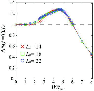
Figure 5: (color online)  Disorder dependence of the pumped charge at $t=T$. We take $T=20$ and $m=0$.

To examine how the pumped charge is enhanced by the disorder, we analyze the real-space dependence of the pumped charge. In Fig. 6, we show the charge distribution at $t=T$ for several different strengths of the disorders. Because the charge pumping mainly occurs around the edges ($x\sim 0,L_{x}-1$), we enlarge the shaded region in Fig. 6(a) and plot the $x$ dependence of the pumped charge measured from the clean limit ($\Delta\tilde{N}(x,t)=\Delta N(x,t,W)-\Delta N(x,t,W=0)$) in Fig. 6(b).

For small disorder ($W=2$), we find that the disorder mainly changes the pumping around the edges and it does not affect the pumping inside of the systems. This enhancement for small disorder can be explained by the mass renormalization effects Chen et al. (2015); Liu et al. (2016); Shapourian and Hughes (2016); Takane (2016), i.e. disorder increases mass term $m$ and widen the length of Fermi arcs. By further increasing the strengths of the disorders, we find that the pumped charge begins to penetrate into the systems. This behavior can be explained as follows: For the strong disorder region, the Fermi arcs at the surfaces begin to mix with the bulk states. This mixing induces the penetration of the Fermi arcs inside the systems, i.e., Fermi arcs begins to have finite width in $x$ direction and induces the charge pumping inside of the systems. This is the reason why the pumped charge is enhanced by the disorder.

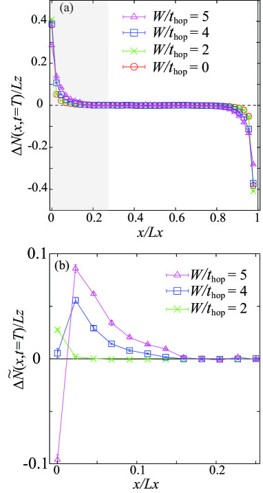
Figure 6: (color online) (a) Charge pumping in the presence of the disorder. We plot $\Delta N(x,t)/L_{z}$ at $t=T$ for several different strengths of disorder. To estimate the errors of the realizations of the disorder, we take five different realizations and regard its standard errors as error bars. We take $L=44$ and $m=0$. (b) Pumped charge measured from the clean limit [$\Delta\tilde{N}(x,t=T)$] in the shaded region in (a). By increasing the strength of the disorder, we find that the pumped charges penetrate into the inside of the system.

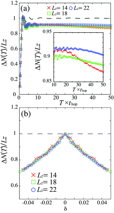
Figure 7: (color online) (a)  $T$ dependence of the charge pumping $\Delta N(t=T)/L_{z}$ at finite doping $\delta=0.01$. We take $m=0$. For comparison, we plot result at zero doping by broken lines. In the inset, we show enlarged figure for $T\geq 10$. (b)Doping dependence of charge pumping for $T=20$. Charge pumping monotonically decrease by doping.

III.3 Effects of doping

In this subsection, we examine the effects of doping on the charge pumping in the Weyl semimetal. First, we examine whether the adiabatic limit of the charge pumping exists for finite doping where the finite density of states exists. In Fig. 7(a), we show $T$ dependence of the pumped charge. At small $T$ ($T\leq 1$), i.e., at the non-adiabatic process, $T$ dependence of the pumped charge is same as that of zero doping. Here, the doping rate is defined as $\delta=\Delta N/N_{s}$, where $\Delta N$ is the number of electrons measured from half filling, i.e., $\Delta N=N_{e}-N_{s}$. In the non-adiabatic region, because the electrons move too fast, low-energy structures of the systems such as the Fermi surfaces do not affect the charge pumping. This is the reason why the pumped charges do not change in the non-adiabatic region.

By taking larger $T$, we find that $T$ dependence of the charge pumping is basically the same as that of the non-doping case, i.e., the large oscillations seen for small $T$ ($T\leq 5$) are suppressed and the pumped charge seems to converge to the constant for $T\leq 20$. However, as shown in the inset in Fig. 7(a), it slightly decreases for $T\geq 20$ and there is considerable system-size dependence. From the available data, it is difficult to identify whether the origin of the decrease is the finite-size effects or not and it is also difficult to accurately estimate the converged pumped charge in the long-time and bulk limit for the doped case. Nevertheless, as we show later, the pumped charge around $T=20$ can capture the essence of the finite doping effects on the charge pumping and can be useful for detecting the remnant of the quantized charge pumping at zero doping. Thus, to examine the doping effects, we use the pumped charge at $T=20$ as a simple estimation of the converged value.

In Fig. 7(b), we show doping dependence of the pumped charge for $T=20$. We find that the pumped charge monotonically decreases for electron and hole doping except for slight oscillations found in small system sizes. This result shows that doping into the Weyl semimetals continuously lowers pumped charge from its quantized values at zero doping. We note that the changes in the pumped charge are induced by the Berry curvature in non-linear dispersions because the Berry curvature in linear dispersions around the Weyl points does not contribute to the pumped charge. We note that the saddle points around the zero doping are located at $E_{\rm saddle}=\pm t_{\rm hop}$ and corresponding doping rate is given by $\delta_{\rm saddle}\sim\pm 0.065.$

We examine the disorder effects of Thouless pumping at finite dopings. In Fig. 8, we plot disorder $W$ dependence of the pumped charge for several different doping rates. At finite doping rates, quantization at zero doping is absent, the pumped charge monotonically increases as a function the disorder strength $W$. By further increasing the disorder, the pumped charge has peaks around $W\sim 4.5$ as in the case of the zero doping. The robustness of the peak structure against the finite doping rates is a characteristic feature of the Weyl semimetal. In the strong disorder region ($W\geq 6$), charge pumping does not depend on the doping rates because the Fermi surfaces are completely smeared out in this region.

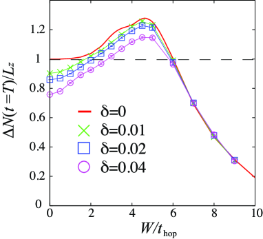
Figure 8: (color online) Disorder $W$ dependence of pumped charge at finite doping. We take $T=20$ and $m=0$.

IV Summary

To summarize, we have introduced the lattice model for the Weyl semimetal in Sec.2.A and have detailed the methods for solving the time-dependent Schrödinger equations by using the fourth-order Suzuki-Trotter decomposition in Sec.2.B. Although the time-dependent Schrödinger equations can be solved by performing the diagonalization of the Hamiltonian at each time step, numerical cost of diagonalization is large and that method can not be applied to the large systems. The Suzuki-Trotter decomposition method does not require the diagonalization of the full Hamiltonian at each time step, numerical cost is dramatically reduced. By using this method, we can perform the Thouless pumping up to the order of $10^{4}$-sites systems.

In Sec. 3.A, we have shown the results of the Thouless pumping for clean limit and zero doping. Although the Weyl semimetal does not have the bulk charge gap, we have found that the Thouless pumping works well for detecting the topological quantization of the Weyl semimetals. By examining the unit time $T$ dependence of the charge pumping, we confirm that the adiabatic charge pumping occurs for larger $T$, typically $T\geq 20$.

In Sec. 3.B, we have examined the disorder effects on the Thouless pumping. We note that the Thouless pumping itself can be applied to the disorder systems without changing the method because we just solve the time-dependent Schrödinger equations in the real space. As a result, we have shown that the quantized pumped charge is robust against small disorder. We have also shown that the pumped charge increases by increasing the disorder for the intermediate strength of disorder. These behaviors are consistent with the previous studies Chen et al. (2015); Liu et al. (2016); Shapourian and Hughes (2016); Takane (2016). This shows that the usefulness of the Thouless pumping for detecting the topological properties in the disordered systems.

We have found that the charge pumping has large system size dependence around $W\sim 3$ as shown in Fig.5, where the transition between Weyl semimetals and diffusive metal is pointed out in the literature Shapourian and Hughes (2016). Thus, this system size dependence may be related to the transition into the diffusive metal. In this study, available system size is limited and it is difficult to perform the accurate finite-size scaling for detecting the signatures of the phase transitions. Systematic calculations for determining the phase transitions is left for future studies.

In Sec. 3.C, we have examined the effects of the doping into the Weyl semimetals. For finite doping rates, we have found that the pumped charge slightly decreases for larger $T$ and it is difficult to accurately estimate the pumped charge in the adiabatic limit. In this paper, we simply use the pumped charge at $T=20$ as a rough estimation of the adiabatic pumping. It is left for future studies to accurately estimate the pumped charge in the adiabatic limit by performing calculations for larger system sizes and larger $T$. By using the pumped charge at $T=20$, we have shown that the remnant of the quantized pumped charge can be detected for finite doping rates. We have also shown that the pumped charge is also enhanced by increasing the disorders for finite doping rates. The peak positions of the charge pumping under disorder do not largely depend on the doping rates.

Our results show that the Thouless pumping is a useful theoretical tool for detecting the topological properties even for the gapless systems such as the Weyl semimetals. This method is also applicable to the doped systems and can capture remnant of the topological properties of the systems through the charge pumping. Because the Thouless pumping only requires the real-time evolution of the ground-state wave functions, it can be applied to the correlated electron systems where it is difficult to obtain the full eigenvectors. For the one-dimensional system, the Thouless pumping for the correlated system is studied in detail Nakagawa et al. (2018). Recent studies Haegeman et al. (2011); Carleo et al. (2012); Ido et al. (2015) show that it is possible to perform the accurate real-time evolutions of the wavefunctions in the correlated quantum many-body systems based on the time-dependent variations principles McLachlan (1964). Studies in this direction are intriguing challenges for clarifying the nature of the correlated topological systems in more than one dimension and our detailed study on the Thouless pumping presented in this paper offers a firm basis for such advanced studies.

Appendix A Thouless pumping in two dimensional Chern insulators

Here, we show the results of the Thouless pumping for the two-dimensional quantum anomalous Hall (QAH) insulators. By simply ignoring the $z$ dependence of the Weyl Hamiltonians, we can obtain the lattice Hamiltonian for the two-dimensional QAH insulators as follows:

$$H_{\rm QAH}=\sum_{\nu=x,y}H_{\nu}+H_{\rm diag},$$ (45)

$$H_{\rm diag}=(2-m)\sum_{j}c_{j}^{\dagger}\sigma_{z}c_{j}+\sum_{j}\epsilon_{j}c_{j}^{\dagger}\sigma_{0}c_{j},$$ (46)

$$\epsilon_{j}\in[-W/2,W/2].$$ (47)

For $m>0$, we obtain the QAH insulator with $\mathcal{C}=1$ and trivial insulator appears for $m<0$. We consider $L=L_{x}=L_{y}$ systems and the pumped charge is given by

$$\Delta N_{\rm 2D}(t)=\sum_{0\leq x<L_{x}/2,y}N(x,y,t)-\sum_{L_{x}/2\leq x<L_{x},y}N(x,y,t)$$ (48)

We note that the charge pumping is quantized as follows:

$$\Delta N_{\rm 2D}(t=T)=2\times\mathcal{C},$$ (49)

where $\mathcal{C}$ is the Chern number.

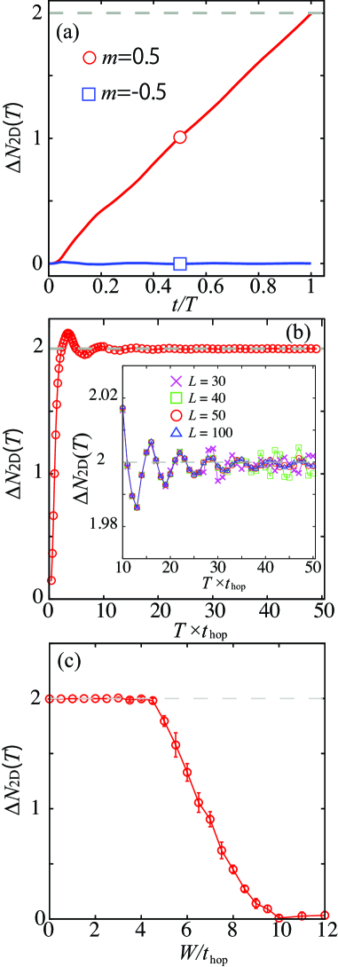
Figure 9: (color online)  (a) Thouless pumping for the Chern insulator ($m=0.5$) and trivial insulator ($m=-0.5$). We take $L=50$ and $T=20$. (b)  $T$ dependence of charge pumping for $L=50$ and $m=0.5$. In the inset, we show the enlarged figure for $T\geq 10$. In the QAH systems, we find that the oscillations in the pumped charge become smaller for larger $T$. (c) Disorder dependence of the pumped charge.

In Fig. 9(a), we show the results of Thouless pumping for $m=0.5$ and $m=-0.5$. In the topologically trivial insulator ($m=-0.5$), the charge pumping does not occur while the charge pumping is quantized for $m=0.5$. Because the Chern number is 1 in this system, the quantized charge pumping becomes 2.

We show $T$-dependence of the $\Delta N_{\rm 2D}(T)$ in Fig.9(b). Similar to the Weyl semimetals, although the oscillation occurs for small $T$ ($T\leq 10$), the charge pumping converges to the quantized value. In the QAH insulators, we only show the results for $L=50$ because size effects are small.

We show the disorder dependence of the $\Delta N_{\rm 2D}(T)$ in Fig.9(c). In contrast to the Weyl semimetals, the charge pumping does not have peak structures. For $W\leq 5$, the pumped charge is quantized and it begins to decrease for $W\geq 5$. This result indicates that the characteristic enhanced charge pumping in the Weyl semimetal is induced by its gapless nature.