A Multiorbital Quantum Impurity Solver for General Interactions and Hybridizations

Abstract

We present a numerically exact Inchworm Monte Carlo method for equilibrium multiorbital quantum impurity problems with general interactions and hybridizations. We show that the method, originally developed to overcome the dynamical sign problem in certain real-time propagation problems, can also overcome the sign problem as a function of temperature for equilibrium quantum impurity models. This is shown in several cases where the current method of choice, the continuous-time hybridization expansion, fails due to the sign problem. Our method therefore enables simulations of impurity problems as they appear in embedding theories without further approximations, such as the truncation of the hybridization or interaction structure or a discretization of the impurity bath with a set of discrete energy levels, and eliminates a crucial bottleneck in the simulation of ab initio embedding problems.

Quantum impurity models describe a small number of strongly interacting confined states coupled to wide noninteracting baths. While originally introduced to address magnetic impurities in metals (Anderson, 1961), they are now predominantly employed in the context of embedding theories such as the dynamical mean field theory (Metzner and Vollhardt, 1989; Georges and Kotliar, 1992; Georges et al., 1996), its variants (Biermann et al., 2003; Maier et al., 2005; Held et al., 2006; Kotliar et al., 2006), and the self-energy embedding theory (Kananenka et al., 2015; Zgid and Gull, 2017). In these theories, the solution of the intractable continuum quantum many-body system describing a correlated material is approximately mapped onto a sequence of effective quantum impurity problems coupled by a self-consistency condition that determines their bath parameters. Evaluating properties of correlated materials then requires repeatedly obtaining the Green’s functions of quantum impurity problems.

Only in the simplest cases can impurity problems be solved at polynomial cost. Examples are impurities comprising only a single interacting orbital, for which powerful continuous-time quantum Monte Carlo (QMC) (Rubtsov and Lichtenstein, 2004; Rubtsov et al., 2005; Werner et al., 2006; Gull et al., 2008, 2011) and renormalization group algorithms (Bulla et al., 2008; Wolf et al., 2014; Stadler et al., 2016) exist. Other examples are systems with high symmetry and/or special interactions. For instance, particle–hole symmetry with local density–density interactions, which allows the solution of interacting impurity problems with hundreds of sites (LeBlanc and Gull, 2013); or systems where the coupling to the baths (the “hybridization”) does not mix the eigenstates of the confined Hamiltonian (i.e. is diagonal in that basis). Everywhere else, the solution of the impurity model either suffers from a “sign problem” that causes an exponential scaling (as a function of temperature, interaction, and number of interacting orbitals) or requires additional approximations, such as the discretization of the continuum of bath states and their approximation with a set of relatively few discrete bath levels (Caffarel and Krauth, 1994; Koch et al., 2008; Zgid et al., 2012; Lu et al., 2014; Shee and Zgid, ; Zhu et al., ).

In the context of embedding simulations of electronic structure problems, these limitations are severe. Many important correlated systems contain transition metal atoms with multiple correlated orbitals. Their symmetries are rarely high enough that only diagonal hybridization is expected, especially when surface problems are studied (Gorelov et al., 2009). Furthermore, the phenomena of interest often only appear at low temperature. As a consequence, practitioners typically neglect the terms generating the sign problem in the Hamiltonian and readjust the remaining parameters by hand. This limits the predictive power of embedding methods and their use in ab-initio frameworks, but enables simulations at temperatures that would otherwise not be accessible. A numerical method able to reach low temperatures for general impurity Hamiltonians without suffering from an exponential slowdown would eliminate the need for these approximations and bridge a central gap in the road to predictive simulations of correlated electron systems.

In this paper, we present an Inchworm QMC method that overcomes the low temperature sign problem in multiorbital impurity models, thereby eliminating these limitations. The method builds on an idea developed to address real-time dynamics of single orbital quantum impurity problems (Cohen et al., 2015; Chen et al., 2017; Antipov et al., 2017; Boag et al., 2018; Dong et al., 2017; Krivenko et al., ), which overcomes the dynamical sign problem, i.e. the exponential scaling as a function of time, in certain nonequilibrium setups (Cohen et al., 2015). A key insight in this regard is that both the dynamical and multiorbital sign problems stem from changing signs in the hybridizations, which the Inchworm method is able to deal with. We emphasize that the method does not present a general solution to the fermion sign problem (i.e. the exponential scaling as a function of impurity size).

Generic model and method

We consider generic impurity Hamiltonians of the form $\hat{H}=\hat{H}_{I}+\hat{H}_{B}+\hat{H}_{IB}.$ Here,

$$\hat{H}_{I} =\sum_{ij\sigma}^{N}\varepsilon_{ij,\sigma}\hat{d}_{i\sigma}^{\dagger}\hat{d}_{j\sigma}+\sum_{ijkl\sigma\sigma^{\prime}}^{N}U_{ijkl}\hat{d}_{i\sigma}^{\dagger}\hat{d}_{k\sigma^{\prime}}^{\dagger}\hat{d}_{l\sigma^{\prime}}\hat{d}_{j\sigma}$$ (1)

is a Hamiltonian on a local Hilbert space with $N$ orbitals and local one-body ($\varepsilon_{ij}$) and two-body ($U_{ijkl}$) terms;

$$\hat{H}_{B} =\int\mathrm{d}k\varepsilon\left(k\right)\hat{b}^{\dagger}\left(k\right)\hat{b}\left(k\right)$$ (2)

is a noninteracting, typically continuous bath Hamiltonian with dispersion $\varepsilon\left(k\right)$; and

$$\hat{H}_{IB} =\sum_{i}\int\mathrm{d}k\left[t_{i}\left(k\right)\hat{b}^{\dagger}\left(k\right)\hat{d}_{i}+\mathrm{h.c.}\right]$$ (3)

is the impurity–bath coupling Hamiltonian with hopping terms $t_{i}\left(k\right)$. The $\hat{d}_{i}^{\left(\dagger\right)}$ and $\hat{b}^{\left(\dagger\right)}\left(k\right)$ destroy (create) particles on the impurity and in the baths, respectively. The computational challenge consists of computing the single-particle imaginary-time Green’s function $G_{ij}\left(\tau\right)=-\left\langle T_{\tau}\hat{d}_{i}\left(\tau\right)\hat{d}_{j}^{\dagger}\left(0\right)\right\rangle$.

The present method of choice, CT-HYB (Werner et al., 2006; Werner and Millis, 2006; Gull et al., 2011), proceeds by expanding the partition function $Z=\text{\text{Tr}}e^{-\beta\hat{H}}$ (with $\beta$ the inverse temperature) into a diagrammatic series in terms of the hybridization, Eq. 3. Using Wick’s theorem, diagrams are combined into determinants (Werner et al., 2006) and stochastically sampled in a random walk procedure (Prokof’ev and Svistunov, 1998; Rubtsov et al., 2005). Green’s functions are measured by eliminating hybridization lines from partition function diagrams (Werner et al., 2006). The method scales exponentially in the number of orbitals $N$, as the local Hamiltonian needs to be diagonalized (Werner and Millis, 2006; Haule, 2007). It scales polynomially in the inverse temperature if the Wick determinants are positive for each diagram. As this is only the case in certain high symmetry situations, the algorithm suffers from a sign problem in general and its scaling is exponential with inverse temperature.

The multiorbital Inchworm method presented in this paper is an imaginary-time adaptation of the real-time formalism of Ref. (Cohen et al., 2015) combined with the multiorbital formulation of CT-HYB described in Ref. (Werner and Millis, 2006). The fundamental objects in the method are imaginary-time impurity propagators $Z(\tau)=\text{Tr}_{B}e^{-\tau\hat{H}}$, where $\text{Tr}_{B}$ denotes a trace over bath states. Propagators are sequentially obtained on a uniform grid $\tau_{n}=n\Delta\tau$ with integer $n$ increasing from 0 to $\frac{\beta}{\Delta\tau}$. The first steps (small $n$) are similar to high temperature simulations and easily performed with CT-HYB. In later steps at larger $n$, the algorithm efficiently expresses $Z\left(\tau_{n}\right)$ in terms of $\left\{\left.Z\left(\tau_{i}\right)\right|0\leq i<n\right\}$.

As has been shown in the context of real-time algorithms (Cohen et al., 2015), this incremental procedure vastly reduces the number of diagrams to be computed and thereby decomposes one large, difficult calculation into many interdependent, easier ones. The technical implementation of the method closely follows the real-time implementation described in detail in Refs. (Cohen et al., 2015), with two changes. First, the propagation direction of real time $t$ is replaced by the orthogonal imaginary time direction $\tau=it.$ Second, the large value of the propagators and partition functions requires normalization with $e^{-\tau\hat{H}_{I}}$ in order to avoid numerical instabilities.

After obtaining the propagators, the Green’s functions are computed according to the procedure detailed in Ref. (Antipov et al., 2017): $Z(\beta)G_{ij}(\tau)$ is obtained in a separate expansion, and $G_{ij}\left(\tau\right)$ extracted by division with $Z\left(\beta\right).$ Implementation details and techniques are otherwise identical to Ref. (Antipov et al., 2017), and fast summation techniques (Boag et al., 2018) can be used. A brief derivation of the algorithm is included in the supplemental materials .

In order to illustrate the power of the algorithm, we focus on two setups that are known to be difficult for state-of-the-art algorithms. Parameters are chosen such that a first set is straightforwardly accessible with current technology; a second set is difficult but possible; and a third set is far out of reach of current methods. Due to the interconnected nature of the Inchworm simulations we choose to compare errors on observables of interest (such as the Green’s function) for a fixed CPU time in each model. Confidence interval estimates (shaded regions in all figures) were obtained from a Jackknife analysis of 5 independent calculations, allowing us to account for nonlinear error propagation and potential error amplification in the Inchworm algorithm.

Spinless Anderson Model

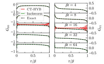
Figure 1: Imaginary-time Green’s function for the spinless Anderson model at temperatures $T=t/4$ (top panel), $T=t/64$ (bottom panel), and for intermediate temperatures indicated. Diagonal (left panels) and off-diagonal (right panels) elements for a small discrete bath (see text) obtained with exact diagonalization (dashed black), CT-HYB (solid red) and Inchworm (solid green). CT-HYB data is only available down to $T=t/16$, and the systematic deviation of the CT-HYB results are indicative of an additional ergodicity problem.

We first examine the two-orbital spinless Anderson model (SAM) (Kashcheyevs et al., 2007; Härtle et al., 2013),

$$\hat{H} =\sum_{i\in\left\{0,1\right\}}\varepsilon_{i}\hat{\text{n}}_{i}+U\hat{\text{n}}_{0}\hat{\text{n}}_{1}-v\left(\hat{d}_{0}^{\dagger}\hat{d}_{1}+\mathrm{h.c}\right)$$ (4)

$$+\sum_{k}\sum_{i\in\left\{0,1\right\}}\varepsilon_{ik}\hat{b}_{ik}^{\dagger}\hat{b}_{ik}-t\sum_{k}\sum_{i\in\left\{0,1\right\}}\left(\hat{d}_{i}^{\dagger}\hat{b}_{ik}+\mathrm{h.c}\right)$$

$$-t^{\prime}\sum_{k}\left(\hat{b}_{0k}^{\dagger}\hat{b}_{1k}+\mathrm{h.c}\right),$$

which is a minimal model exposing the exponential scaling issues in CT-HYB (Parcollet et al., 2015; Seth et al., 2016). Here $i$ enumerates the two (spinless) orbitals $0$ and $1$ at local level energy $\varepsilon_{i}$. Each orbital is connected to its own bath orbitals (enumerated by quantum numbers $i$ and $k$ and at level energy $\varepsilon_{ik}$) with coupling $t$ and to the other orbital with coupling $v$. The density in orbital $i$ is $\hat{n}_{i}=\hat{d}_{i}^{\dagger}\hat{d}_{i}$ and $U$ is a local inter-orbital interaction strength. Pairs of same-$k$ orbitals in the two baths are connected with a hopping $t^{\prime}$. Here we choose two degenerate, discrete bath states per orbital at zero energy ($\varepsilon_{ik}=0$ for $i,k=0,1$). The remaining parameters are set to $\varepsilon_{i}=0$, $U=4t$, $v=t$ and $t^{\prime}=\frac{3}{2}t$. This finite model can be diagonalized exactly, providing an independent benchmark for comparison. The mixing of different bath orbitals, here generated by $t^{\prime},$ is typical for multiorbital embedding setups and, in CT-HYB, results in a severe sign problem.

Fig. 1 shows the exact Green’s functions (dashed black line) along with the results from CT-HYB (red) and Inchworm (green). The parameters were chosen such that the sign problem in CT-HYB is particularly large (Parcollet et al., 2015; Seth et al., 2016). For symmetry reasons $G_{00}=G_{11}$ and $G_{01}=G_{10}$; we therefore only show $G_{00}$ (left panels) and $G_{01}$ (right panels). Note that while $G_{00}$ is strictly negative and convex, $G_{01}$ is neither. Six temperatures ($\beta t=4,8,16,32$, and $\beta t=64$) are shown, in decreasing order from the top to the bottom panels. CT-HYB data are only available for $\beta t=4,8,$ and $\beta t=16.$ The time discretization parameter $\Delta\tau$ was set to $\beta/80$, and the maximum Inchworm diagram order was restricted to 8 (Cohen et al., 2015). In this simulation, the maximum order was rarely reached and, as also evidenced by comparison with the exact result, diagram truncation and discretization errors are smaller than stochastic errors. Inchworm (CT-HYB) calculations were run for 0.5K (12K) core hours; both algorithms are trivially parallelizable.

At high temperature (top two panels), all methods agree. Statistical errors are slightly larger for CT-HYB at the second temperature. However, at $\beta t=16$, CT-HYB breaks down, exhibiting both large errors and additional ergodicity issues. For the same parameters, the Inchworm method remains accurate and consistent with the exact reference, and results remain correct down to the lowest temperature shown, $\beta t=64$. This behavior is generic for models with off-diagonal (bath-mixing) hybridizations.

Kanamori Model

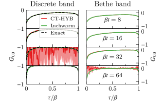
Figure 2: Diagonal imaginary-time Green’s function for the Kanamori model at temperature $T=t/8$ (top panel), $T=t/64$ (bottom panel), and intermediate temperatures $T=t/16$ and $T=t/32$, for a discrete band (left panels) and a semi-circular band with $t=1$. Results from CT-HYB (solid red) and Inchworm (solid green), along with exact diagonalization where available (black, left panel only).

We now consider the two-orbital Kanamori model with spherically symmetric interactions, which has two orbitals with two spins each. Kanamori models exhibit interesting non-Fermi-liquid “spin freezing” (Werner et al., 2008) and “Hund’s metal” physics (Yin et al., 2011; de’ Medici et al., 2011; Georges et al., 2013), and are frequently considered in multiorbital DMFT simulations of transition metal compounds with cubic symmetry. The two-orbital variant with local Hamiltonian

$$\hat{H} =U\sum_{i\in\left\{0,1\right\}}\hat{n}_{i\downarrow}\hat{n}_{i\uparrow}+\left(U-2J\right)\sum_{i\neq j}\hat{n}_{i\downarrow}\hat{n}_{j\uparrow}$$ (5)

$$+\left(U-3J\right)\sum_{i>j,\sigma}\hat{n}_{i\sigma}\hat{n}_{j\sigma}$$

$$+J\sum_{i\neq j}\left(\hat{d}_{i\uparrow}^{\dagger}\hat{d}_{j\downarrow}^{\dagger}\hat{d}_{i\downarrow}\hat{d}_{j\uparrow}+\mathrm{h.c.}\right)$$

is commonly used for $e_{g}$ bands in correlated 3d or 4d orbitals. The local part of the model is parameterized by the Coulomb $U$ and Hund’s $J$ interaction parameters, which we set to $U=2t$ and $J=0.2t$. The “spin-exchange” and “pair-hopping” terms in the last line are the only non-density–density terms and—although frequently neglected—have an important effect on the physics (Werner et al., 2008). Within DMFT, this local Hamiltonian hybridizes with a bath modeled by a frequency- and orbital-dependent hybridization function $\Delta_{ij}(\omega)$ that generically mixes different orbitals.

In the following, we consider two hybridization functions $\Delta_{ij}=\left(\delta_{ij}+r\left(1-\delta_{ij}\right)\right)t^{2}\mathcal{G}\left(\omega\right)$, where $r$ controls the relative size of off-diagonal elements and $a$ controls the overall coupling strength. The first hybridization is an exactly solvable discrete band $\mathcal{G}\left(\omega\right)=\sum_{k}\delta\left(\omega-\varepsilon_{k}\right)$ with two levels $\varepsilon_{k}\in\left\{\pm 2.3t\right\}$ per spin-orbital, at $r=\frac{1}{2}$ and $a=1$. The second hybridization describes coupling to a continuous semicircular band $\mathcal{G}\left(\omega\right)=\frac{2}{\pi D^{2}}\sqrt{D^{2}-\omega^{2}}$, where the half bandwidth is $D$. Here we set $r=1$, $D=2t$ to consider a band as it occurs in the solution of the dynamical mean field equations in the infinite coordination number limit on a Bethe lattice.

Fig. 2 shows the diagonal, same-spin Green’s function elements, $G_{00}\left(\tau\right)\equiv G_{i\sigma,i\sigma}\left(\tau\right)$. The discrete case (left panels) can be exactly diagonalized (dashed black curves), but for the continuous case (right panels) no analytical results are available. The sign problem in this system is not as severe as in the SAM, and we can therefore present CT-HYB results down to half the lowest temperature in Fig. 1. The numerical parameters and statistical analysis are as in the SAM. All Inchworm (CT-HYB) calculations were run for 1.5K (3K) core hours.

While CT-HYB performs reasonably well at high temperature, it breaks down for both band types as $T$ is lowered to $\beta t=32$ (left panels) and $\beta t=64$ (right panels). Inchworm shows controlled results for all cases in both models, though small deviations between Inchworm and the exact solution, due to discretization errors, are visible in the bottom left panel. We verified that these deviations can easily be removed by decreasing $\Delta\tau$ (not shown).

Scaling analysis

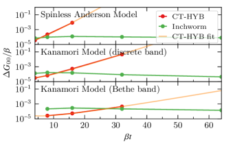
Figure 3: Scaling analysis. Mean absolute deviation from exact result (top two panels, SAM and discrete Kanamori models) and statistical standard errors (bottom panel, continuous Bethe band Kanamori model) divided by inverse temperature $\beta$, as a function of $\beta$. CT-HYB (red) and Inchworm (green) results are shown along with exponential fits for CT-HYB (light red).

The results presented so far are qualitative, insofar as CT-HYB breaks down in several cases where Inchworm does not. To gain additional insight into the nature of the observed breakdown and the relative merits of the two methods, we present a quantitative error analysis in Fig. 3. We plot Green’s function error estimates for the three different models as a function of the inverse temperature $\beta$. The errors are divided by $\beta$ and shown on a logarithmic scale. For the SAM and the discrete Kanamori models (two upper panels), the error estimates are given by the absolute value of difference from the exact result, $\Delta G\equiv\left|G-G_{\mathrm{\text{Exact}}}\right|$; they therefore also take into account any systematic bias the Monte Carlo methods might exhibit. In the lower panel, for the Kanamori model coupled to a continuous Bethe band, no exact result is available. The errors are therefore obtained from a Jackknife analysis on 5 independent calculations, and account only for the magnitude of variation between these runs. We note that the absolute value of the errors is of course implementation dependent. Here we used the highly optimized ALPS CT-HYB code (Shinaoka et al., 2017; Gaenko et al., 2017; Wallerberger et al., ), and an Inchworm implementation written in C++.

In all cases shown, ALPS CT-HYB is more accurate than our Inchworm implementation for high temperature. However, as a function of $\beta,$ the $\frac{\Delta G}{\beta}$ obtained within CT-HYB is at least exponential in $\beta$ (see fits in Fig. 3, which are extrapolated beyond where CT-HYB errors can be reliably obtained). This exponential scaling is a consequence of the presence of a sign problem. In contrast, the $\frac{\Delta G}{\beta}$ obtained with the Inchworm method is essentially flat, implying a linear scaling in inverse temperature. This means that, for the systems presented, the Inchworm method presents a solution to the sign problem as a function of temperature and allows access to temperatures that are much lower than what is possible with CT-HYB. For example, Fig. 3 shows that in the Bethe case, obtaining a result of comparable quality to our Inchworm data at $\beta=64$ with ALPS CT-HYB would take ~$3\times 10^{9}$ core hours or ~342K core years.

The linear scaling of the Inchworm method should be interpreted only as a lower bound: at even lower temperatures, a finer time discretization or a generalization to a non-uniform grid will be needed to maintain accuracy. We expect this to result in a low-order (but more than linear) polynomial scaling in the inverse temperature . We emphasize again that the method is not a general solution of the fermion sign problem, as it remains explicitly exponential in the number of interacting orbitals.

In conclusion,

we present an equilibrium multiorbital quantum impurity solver based on the Inchworm method. We show, for two generic scenarios, that the method avoids the exponential scaling with inverse temperature observed in other methods and thereby presents a “solution” to this particular class of sign problems. A comparison to the state-of-the-art method, CT-HYB, shows that parameter regimes are now accessible that were previously out of reach of numerically exact quantum impurity solvers.

Our Inchworm impurity solver addresses a critical need for numerically exact multiorbital quantum impurity solvers that can treat both generic four-fermion interaction terms and generalized non-diagonal hybridization functions. This need stems from embedding constructions such as the DMFT or the self-energy embedding theory, where hybridization functions typically arise as continuous multiorbital functions in frequency space and interactions are not of the density–density type. By being able to solve such impurity problems without introducing additional artificial discretizations of the bath orbitals, and without further truncating and approximating the hybridization and interaction structure, the method bridges an important gap on the route to controlled ab-initio many-body embedding theories.