Universality and individuality in neural dynamics across large populations of recurrent networks
Abstract
Task-based modeling with recurrent neural networks (RNNs) has emerged as a popular way to infer the computational function of different brain regions. These models are quantitatively assessed by comparing the low-dimensional neural representations of the model with the brain, for example using canonical correlation analysis (CCA). However, the nature of the detailed neurobiological inferences one can draw from such efforts remains elusive. For example, to what extent does training neural networks to solve common tasks uniquely determine the network dynamics, independent of modeling architectural choices? Or alternatively, are the learned dynamics highly sensitive to different model choices? Knowing the answer to these questions has strong implications for whether and how we should use task-based RNN modeling to understand brain dynamics. To address these foundational questions, we study populations of thousands of networks, with commonly used RNN architectures, trained to solve neuroscientifically motivated tasks and characterize their nonlinear dynamics. We find the geometry of the RNN representations can be highly sensitive to different network architectures, yielding a cautionary tale for measures of similarity that rely on representational geometry, such as CCA. Moreover, we find that while the geometry of neural dynamics can vary greatly across architectures, the underlying computational scaffold—the topological structure of fixed points, transitions between them, limit cycles, and linearized dynamics—often appears universal across all architectures.
1 Introduction
The computational neuroscience community is increasingly relying on deep learning both to directly model large-scale neural recordings [1, 2, 3] as well to train neural networks on computational tasks and compare the internal dynamics of such trained networks to measured neural recordings [4, 5, 6, 7, 8, 9]. For example, several recent studies have reported similarities between the internal representations of biological and artificial networks [5, 10, 11, 12, 13, 14, 15, 16]. These representational similarities are quite striking since artificial neural networks clearly differ in many ways from their much more biophysically complex natural counterparts. How then, should we scientifically interpret the striking representational similarity of biological and artificial networks, despite their vast disparity in biophysical and architectural mechanisms?
A fundamental impediment to achieving any such clear scientific interpretation lies in the fact that infinitely many model networks may be consistent with any particular computational task or neural recording. Indeed, many modern applications of deep learning utilize a wide variety of recurrent neural network (RNN) architectures [17, 18, 19, 20], initialization strategies [21] and regularization terms [22, 23]. Moreover, new architectures continually emerge through large-scale automated searches [24, 25, 26]. This dizzying set of modelling degrees of freedom in deep learning raises fundamental questions about how the degree of match between dynamical properties of biological and artificial networks varies across different modelling choices used to generate RNNs.
For example, do certain properties of RNN dynamics vary widely across individual architectures? If so, then a high degree of match between these properties measured in both an artificial RNN and a biological circuit might yield insights into the architecture underlying the biological circuit’s dynamics, as well as rule out other potential architectures. Alternatively, are other properties of RNN dynamics universal across many architectural classes and other modelling degrees of freedom? If so, such properties are interesting neural invariants determined primarily by the task, and we should naturally expect them to recur not only across diverse classes of artificial RNNs, but also in relevant brain circuits that solve the same task. The existence of such universal properties would then provide a satisfying explanation of certain aspects of the match in internal representations between biological and artificial RNNs, despite many disparities in their underlying mechanisms.
Interestingly, such universal properties can also break the vast design space of RNNs into different universality classes, with these universal dynamical properties being constant within classes, and varying only between classes. This offers the possibility of theoretically calculating or understanding such universal properties by analyzing the simplest network within each universality class111This situation is akin to that in equilibrium statistical mechanics in which physical materials as disparate as water and ferromagnets have identical critical exponents at second order phase transitions, by virtue of the fact that they fall within the same universality class [27]. Moreover, these universal critical exponents can be computed theoretically in the simplest model within this class: the Ising model.. Thus a foundational question in the theory of RNNs, as well as in their application to neuroscientific modelling, lies in ascertaining which aspects of RNN dynamics vary across different architectural choices, and which aspects—if any—are universal across such choices.
Theoretical clarity on the nature of individuality and universality in nonlinear RNN dynamics is largely lacking222Although Feigenbaum’s analysis [28] of period doubling in certain 1D maps might be viewed as an analysis of 1D RNNs., with some exceptions [29, 30, 31, 32]. Therefore, with the above neuroscientific and theoretical motivations in mind, we initiate an extensive numerical study of the variations in RNN dynamics across thousands of RNNs with varying modelling choices. We focus on canonical neuroscientifically motivated tasks that exemplify basic elements of neural computation, including the storage and maintenance of multiple discrete memories, the production of oscillatory motor-like dynamics, and contextual integration in the face of noisy evidence [33, 4].
To compare internal representations across networks, we focused on comparing the geometry of neural dynamics using common network similarity measures such as singular vector canonical correlation analysis (SVCCA) [34] and centered kernel alignment (CKA) [35]. We also used tools from dynamical systems analysis to extract more topological aspects of neural dynamics, including fixed points, limit cycles, and transition pathways between them, as well as the linearized dynamics around fixed points [33]. We focused on these approaches because comparisons between artificial and biological network dynamics at the level of geometry, and topology and linearized dynamics, are often employed in computational neuroscience.
Using these tools, we find that different RNN architectures trained on the same task exhibit both universal and individualistic dynamical properties. In particular, we find that the geometry of neural representations varies considerably across RNNs with different nonlinearities. We also find surprising dissociations between dynamical similarity and functional similarity, whereby trained and untrained architectures of a given type can be more similar to each other than trained architectures of different types. This yields a cautionary tale for using SVCCA or CKA to compare neural geometry, as these similarity metrics may be more sensitive to particular modeling choices than to overall task performance. Finally, we find considerably more universality across architectures in the topological structure of fixed points, limit cycles, and specific properties of the linearized dynamics about fixed points. Thus overall, our numerical study provides a much needed foundation for understanding universality and individuality in network dynamics across various RNN models, a question that is both of intrinsic theoretical interest, and of importance in neuroscientific applications.
2 Methods
2.1 Model Architectures and Training Procedure
We define an RNN by an update rule, , where denotes some nonlinear function of the network state vector and the network input . Here, is an integer index denoting discrete time steps. Given an initial state, , and a stream of inputs, , , , , the RNN states are recursively computed, , , , . The model predictions are based on a linear readout of these state vector representations of the input stream. We studied 4 RNN architectures, the vanilla RNN (Vanilla), the Update-Gate RNN (UGRNN; [20]), the Gated Recurrent Unit (GRU; [18]), and the Long-Short-Term-Memory (LSTM; [17]). The equations for these RNNs can be found in Appendix A. For each RNN architecture we modified the (non-gate) point-wise activation function to be either rectified linear (relu) or hyperbolic tangent (tanh). The point-wise activation for the gating units is kept as a sigmoid.
We trained networks for every combination of the following parameters: RNN architecture (Vanilla, UGRNN, LSTM, GRU), activation (relu, tanh), number of units/neurons (64, 128, 256), and L2 regularization (1e-5, 1e-4, 1e-3, 1e-2). This yielded = 96 unique configurations. For each one of these configurations, we performed a separate random hyperparameter search over gradient clipping values [22] (logarithmically spaced from 0.1 to 10) and the learning rate schedule parameters. The learning rate schedule is an exponentially decaying schedule parameterized by the initial rate (with search range from 1e-5 to 0.1), decay rate (0.1 to 0.9), and momentum (0 to 1). All networks were trained using stochastic gradient descent with momentum [36, 37] for 20,000 iterations with a batch size of 64. For each network configuration, we selected the best hyperparameters using a validation set. We additionally trained each of these configurations with 30 random seeds, yielding 2,880 total networks for analysis for each task. All networks achieve low error; histograms of the final loss values achieved by all networks are available in Appendix C.
2.2 Tasks
We used three canonical tasks that have been previously studied in the neuroscience literature:
-bit flip-flop
Following [33], RNNs were provided inputs taking discrete values in . The RNN has outputs, each of which is trained to remember the last non-zero input on its corresponding input. Here we set , so e.g. output 2 remembers the last non-zero state of input 2 (+1 or -1), but ignores inputs 1 and 3. We set the number of time steps, , to 100, and the flip probability (the probability of any input flipping on a particular time step) to 5%.
Frequency-cued sine wave
Following [33], RNNs received a static input, , and were trained to produce a unit amplitude sine wave, , whose frequency is proportional to the input: . We set and (5 simulated seconds total).
Context-dependent integration (CDI)
Following previous work [4], RNNs were provided with static context inputs and time-varying white noise input streams. On each trial, all but one context input was zero, thus forming a one-hot encoding indicating which noisy input stream of length should be integrated. The white noise input was sampled from at each time step, with sampled uniformly between -1 and 1 and kept static across time for each trial. RNNs were trained to report the cumulative sum of the cued white-noise input stream across time. Here, we set and .
2.3 Assessing model similarity
The central questions we examined were: how similar are the representations and dynamics of different RNNs trained on the same task? To address this, we use approaches that highlight different but sometimes overlapping aspects of RNN function:
SVCCA and CKA to assess representational geometry
We quantified similarity at the level of representational geometry [38]. In essence, this means quantifying whether the responses of two RNNs to the same inputs are well-aligned by some kind of linear transformation.
We focused on singular vector canonical correlations analysis (SVCCA; [34]), which has found traction in both neuroscience [12] and machine learning communities [39, 15]. SVCCA compares representations in two steps. First, each representation is projected onto their top principal components to remove the effect of noisy (low variance) directions. Typically, the number of components is chosen to retain ~95% of the variance in the representation. Then, canonical correlation analysis (CCA) is performed to find a linear transformation that maximally correlates the two representations. This yields correlation coefficients, , providing a means to compare the two datasets, typically by averaging or summing the coefficients (see Appendix D for further details).
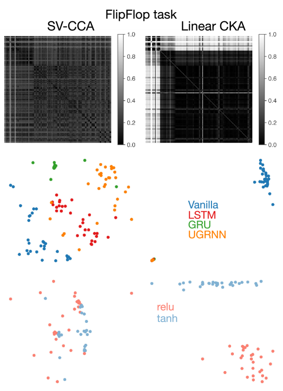
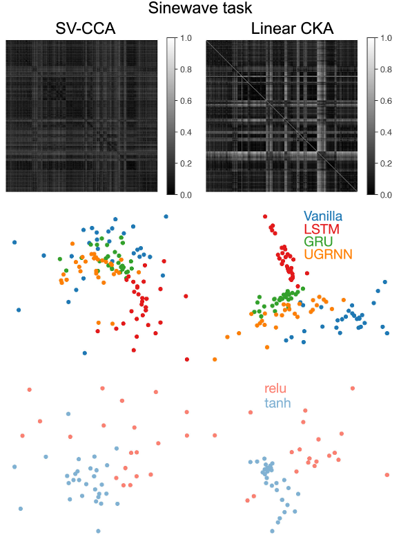
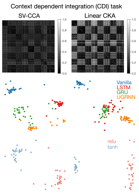
In addition to SVCCA, we explored a related metric, centered kernel alignment (CKA; [35]). CKA is related to SVCCA in that it also suppresses low variance directions, however CKA weights the components proportional to the singular value (as opposed to removing some completely). We found that using SVCCA and CKA yielded similar results for the purposes of determining whether representations cluster by architecture or activation function so we present SVCCA results in the main text but provide a comparison with CKA in Appendix E.
Fixed point topology to assess computation
An alternative perspective to representational geometry for understanding computation in RNNs is dynamics. We studied RNN dynamics by reducing their nonlinear dynamics to linear approximations. Briefly, this approach starts by optimizing to find the fixed points of an RNN such that . We use the term fixed point to also include approximate fixed points, which are not truly fixed but are nevertheless very slow on the time scale of the task.
We set the input () to be static when finding fixed points. These inputs can be thought of as specifying different task conditions. In particular, the static command frequency in the sine wave task and the hot-one context signal in the CDI task are examples of such condition specifying inputs. Note however, that dimensions of that are time-varying are set to in . In particular, the dimensions of the input that represent the input pulses in the -bit memory task and the white noise input streams in the CDI task are set to in .
Numerical procedures for identifying fixed points are discussed in [33, 40]. Around each fixed point, the local behavior of the system can be approximated by a reduced system with linear dynamics:
where denotes the Jacobian of the RNN update rule. We studied these linearized systems using the eigenvector decomposition for non-normal matrices (see Appendix B for the eigenvector decomposition). In this analysis, both the topology of the fixed points and the linearizations around those fixed points become objects of interest.
Visualizing similarity with multi-dimensional scaling
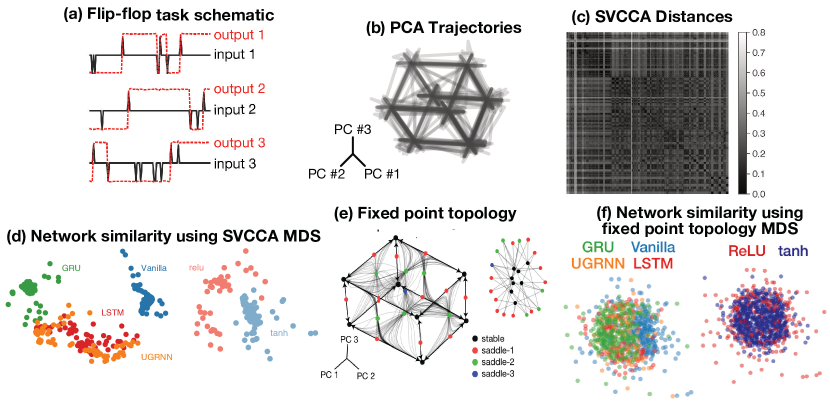
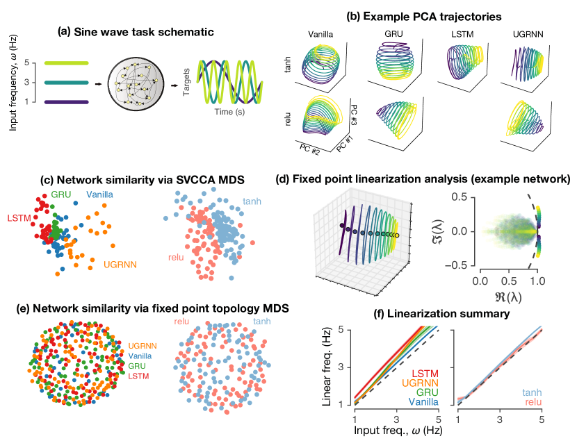
For each analysis, we computed network similarity between all pairs of network configurations for a given task, yielding a large (dis-)similarity matrix for each task (for example, we show this distance matrix for the flip-flop task in Fig. 1c). To visualize the structure in these matrices, we used multi-dimensional scaling (MDS) [41] to generate a 2D projection which we used for visualization (Fig. 1d and f, Fig. 2c and e, Fig. 3c and d). For visualization purposes, we separate plots colored by RNN architecture (for a fixed nonlinearity, tanh) and nonlinearity (for a fixed architecture, Vanilla).
3 Results
The major contributions in this paper are as follows. First, we carefully train and tune large populations of RNNs trained on several canonical tasks relating to discrete memory [33], pattern generation [33], and analog memory and integration [4]. Then, we show that representational geometry is sensitive to model architecture (Figs. 1-3). Next, we show all RNN architectures, including complex, gated architectures (e.g. LSTM and GRU) converge to qualitatively similar dynamical solutions, as quantified by the topology of fixed points and corresponding linearized dynamics (Figs. 1-3). Finally, we highlight a case where SVCCA is not necessarily indicative of functional similarity (Fig. 4).
3.1 3-bit discrete memory
We trained RNNs to store and report three discrete binary inputs (Fig. 1a). In Fig. 1b, we use a simple “probe input” consisting of a series of random inputs to highlight the network structure. Across all network architectures the resulting trajectories roughly trace out the corners of a three-dimensional cube. While these example trajectories look qualitatively similar across architectures, SVCCA revealed systematic differences. This is visible in the raw SVCCA distance matrix (Fig. 1c), as well as in low-dimensional linear embeddings achieved by applying multi-dimensional scaling (MDS) (Fig. 1d) created using the SVCCA distance matrix.
To study the dynamics of these networks, we ran an optimization procedure [40] to numerically identify fixed points for each trained network (see Methods). A representative network is shown in Fig. 1e (left). The network solves the task by encoding all possible outputs as 8 stable fixed points. Furthermore, there are saddle points with one, two, or three unstable dimensions (see caption), which route the network activity towards the appropriate stable fixed point for a given input.
We devised an automated procedure to quantify the computational logic of the fixed point structure in Fig. 1e that effectively ignored the precise details in the transient dynamics and overall geometry of the 3D cube evident in the PCA trajectories. Specifically, we distilled the dynamical trajectories into a directed graph, with nodes representing fixed points, and weighted edges representing the probability of moving from one fixed point to another when starting the initial state a small distance away from the first fixed point. We did this 100 times for each fixed point, yielding a probability of transitioning from one fixed point to another. As expected, stable fixed points have no outgoing edges, and only have a self-loop. All unstable fixed points had two or more outgoing edges, which are directed at nearby stable fixed points. We constructed a fixed point graph for each network and used the Euclidean distance between the graph connectivity matrices to quantify dis-similarity333While determining whether two graphs are isomorphic is a challenging problem in general, we circumvented this issue by lexographically ordering the fixed points based on the RNN readout. Networks with different numbers of fixed points than the modal number were discarded (less than 10% of the population).. These heteroclinic orbits are shown in Fig. 1e, light black trajectories from one fixed point to another. Using this topological measure of RNN similarity, we find that all architectures converge to very similar solutions as shown by an MDS embedding of the fixed point graph (Fig. 1f).
3.2 Sine wave generation
We trained RNNs to convert a static input into a sine wave, e.g. convert the command frequency to (Fig. 2a). Fig. 2b shows low-dimensional trajectories in trained networks across all architectures and nonlinearities (LSTM with ReLU did not train effectively, so we excluded it). Each trajectory is colored by the input frequency. Furthermore, all trajectories followed a similar pattern: oscillations occur in a roughly 2D subspace (circular trajectories), with separate circles for each frequency input separated by a third dimension. We then performed an analogous series of analyses to those used in the previous task. In particular, we computed the SVCCA distances (raw distances not shown) and used those to create an embedding of the network activity (Fig. 2c) as a function of either RNN architecture or activation. These SVCCA MDS summaries show systematic differences in the representations across both architecture and activation.
Moving to the analysis of dynamics, we found for each input frequency a single input-dependent fixed point (Fig. 2d, left). We studied the linearized dynamics around each fixed point and found a single pair of imaginary eigenvalues, representing a mildly unstable oscillatory mode whose complex angle aligned well with the input frequency (Fig. 2d, right). We compared the frequency of the linear model to the input frequency and found generally good alignment. We averaged the linear frequency across all networks within architecture or activation and found small, but systematic differences (Fig. 2f). Embeddings of the topological structure of the input-dependent fixed points did not reveal any structure that systematically varied by architecture or activation (Fig. 2e).
3.3 Context-dependent integration (analog memory)
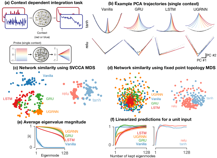
We trained an RNN to contextually integrate one of two white noise input streams, while ignoring the other (Fig. 3a). We then studied the network representations by delivering a set of probe inputs (Fig. 3a). The 3D PCA plots are shown in Fig. 3b, showing obvious differences in representational geometry as a function of architecture and activation. The MDS summary plot of the SVCCA distances of the representations is shown in Fig. 3c, again showing systematic clustering as a function of architecture (left) and activation (right). We also analyzed the topology of the fixed points (black dots in Fig. 3b) to assess how well the fixed points approximated a line attractor. We quantified this by generating a graph with edges between fixed points that were nearest neighbors. This resulted in a graph for each line attractor in each context, which we then compared using Euclidean distance and embedded in a 2D space using MDS (Fig. 3d). The MDS summary plot did not cluster strongly by architecture, but did cluster based on activation.
We then studied the linearized dynamics around each fixed point (Fig. 3e,f). We focused on a single context, and studied how a unit magnitude relevant input (as opposed to the input that should be contextually ignored) was integrated by the linear system around the nearest fixed point. This was previously studied in depth in [4]. Here we were interested in differences in integration strategy as a function of architecture. We found similar results to [4] for the vanilla RNN, which integrated the input using a single linear mode with an eigenvalue of 1, with input coming in on the associated left eigenvector and represented on the associated right eigenvector. Examination of all linearized dynamics averaged over all fixed points within the context showed that different architectures had a similar strategy, except that the gated architectures had many more eigenvalues near 1 (Fig. 3e) and thus used a high-dimensional strategy to accomplish the same goal as the vanilla RNN does in 1 dimension. We further studied the dimensionality by systematically zeroing out eigenvalues from smallest to largest to discover how many linear modes were necessary to integrate a unit magnitude input, compared to the full linear approximation (Fig. 3f). These results show that all of the networks and architectures use essentially the same integration strategy, but systematically vary by architecture in terms of the number of modes they employ. To a lesser degree they also vary some in the amount the higher order terms contribute to the solution, as shown by the differences away from an integral of 1 for a unit magnitude input, for the full linearized system with no modes zeroed out (analogous to Fig. 2f).
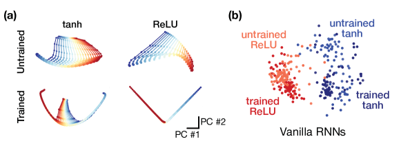
Finally, to highlight the difficulty of using CCA-based techniques to compare representational geometry in simple tasks, we used the inputs of the context-dependent integrator task to drive both trained and untrained vanilla RNNs (Fig. 4). We found that the average canonical correlation between trained and untrained networks can be larger than between trained RNNs with different nonlinearities. The summary MDS plot across many RNNs shows that the two clusters of untrained and trained relu networks are closer together than the two clusters of trained tanh networks Fig. 4b.
4 Related Work
Researchers are beginning to study both empirically and theoretically how deep networks may show universal properties. For example, [32] proved that representational geometry is a universal property amongst all trained deep linear networks that solve a task optimally, with smallest norm weights. Also, [42, 43] studied how expressive capacity increases with network depth and width. Work in RNNs is far more preliminary, though it is well known that RNNs are universal approximators of dynamical systems [44]. More recently, the per-parameter capacity of RNNs was found to be remarkably similar across various RNN architectures [20]. The authors of [45] studied all the possible topological arrangements of fixed points in a 2D continuous-time GRU, conjecturing that dynamical configurations such as line or ring attractors that require an infinite number of fixed points can only be created in approximation, even in GRUs with more than two dimensions.
Understanding biological neural systems in terms of artificial dynamical systems has a rich tradition [46, 47, 48, 49]. Researchers have attempted to understand optimized neural networks with nonlinear dynamical systems techniques [33, 50] and to compare those artificial networks to biological circuits [4, 12, 51, 52, 53, 13, 14].
Previous work has studied vanilla RNNs in similar settings [33, 4, 54], but has not systematically surveyed the variability in network dynamics across commonly used RNN architectures, such as LSTMs [17] or GRUs [18], nor quantified variations in dynamical solutions over architecture and nonlinearity, although [16] considers many issues concerning how RNNs may hold memory. Finally, there has been a recent line of work comparing artificial network representations to neural data [1, 2, 3, 10, 11, 12]. Investigators have been studying ways to improve the utility of CCA-based comparison methods [34, 55], as well as comparing CCA to other methods [35].
5 Discussion
In this work we empirically study aspects of individuality and universality in recurrent networks. We find individuality in that representational geometry of RNNs varies significantly as a function of architecture and activation function (Fig. 1d, 2c, 3c). We also see hints of universality: the fixed point topologies show far less variation across networks than the representations do (Fig. 1f, 2e, 3d). Linear analyses also showed similar solutions, e.g. essentially linear oscillations for the sine wave task (Fig. 2f) and linear integration in the CDI task (Fig. 3f). However, linear analyses also showed variation across architectures in the dimensionality of the solution to integration (Fig. 3e).
While the linear analyses showed common computational strategies across all architectures (such as a slightly unstable oscillation in the linearized system around each fixed point), we did see small systematic differences that clustered by architecture (such as the difference between input frequency and frequency of oscillatory mode in the linearized system). This indicates that another aspect of individuality appears to be the degree to which higher order terms contribute to the total solution.
The fixed point analysis discussed here has one major limitation, namely that the number of fixed points must be the same across networks that are being compared. For the three tasks studied here, we found that the vast majority of trained networks did indeed have the same number of fixed points for each task. However, an important direction for future work is extending the analysis to be more robust with respect to differing numbers of fixed points.
In summary, we hope this empirical study begins a larger effort to characterize methods for comparing RNN dynamics, building a foundation for future connections of biological circuits and artificial neural networks.
Acknowledgments
The authors would like to thank Jeffrey Pennington, Maithra Raghu, Jascha Sohl-Dickstein, and Larry Abbott for helpful feedback and discussions. MDG was supported by the Stanford Neurosciences Institute, the Office of Naval Research Grant #N00014-18-1-2158.
References
- [1] Lane McIntosh et al. “Deep Learning Models of the Retinal Response to Natural Scenes” In Advances in Neural Information Processing Systems 29 Curran Associates, Inc., 2016, pp. 1369–1377 URL: http://papers.nips.cc/paper/6388-deep-learning-models-of-the-retinal-response-to-natural-scenes.pdf
- [2] Niru Maheswaranathan et al. “Deep learning models reveal internal structure and diverse computations in the retina under natural scenes” In bioRxiv Cold Spring Harbor Laboratory, 2018, pp. 340943
- [3] Chethan Pandarinath et al. “Inferring single-trial neural population dynamics using sequential auto-encoders” In Nature Methods 15.10, 2018, pp. 805–815 DOI: 10.1038/s41592-018-0109-9
- [4] Valerio Mante, David Sussillo, Krishna V. Shenoy and William T. Newsome “Context-dependent computation by recurrent dynamics in prefrontal cortex” Article In Nature 503 Nature Publishing Group, a division of Macmillan Publishers Limited. All Rights Reserved. SN -, 2013, pp. 78
- [5] Alexander J E Kell et al. “A Task-Optimized Neural Network Replicates Human Auditory Behavior, Predicts Brain Responses, and Reveals a Cortical Processing Hierarchy” In Neuron 98.3 Elsevier, 2018, pp. 630–644.e16 DOI: 10.1016/j.neuron.2018.03.044
- [6] Rishi Rajalingham et al. “Large-Scale, High-Resolution Comparison of the Core Visual Object Recognition Behavior of Humans, Monkeys, and State-of-the-Art Deep Artificial Neural Networks” In Journal of Neuroscience 38.33 Society for Neuroscience, 2018, pp. 7255–7269 DOI: 10.1523/JNEUROSCI.0388-18.2018
- [7] Christopher J Cueva and Xue-Xin Wei “Emergence of grid-like representations by training recurrent neural networks to perform spatial localization” In arXiv preprint arXiv:1803.07770, 2018
- [8] Andrea Banino et al. “Vector-based navigation using grid-like representations in artificial agents” In Nature 557.7705 Nature Publishing Group, 2018, pp. 429
- [9] Stefano Recanatesi et al. “Predictive learning extracts latent space representations from sensory observations” In bioRxiv Cold Spring Harbor Laboratory, 2019 DOI: 10.1101/471987
- [10] Daniel L.. Yamins et al. “Performance-optimized hierarchical models predict neural responses in higher visual cortex” In Proceedings of the National Academy of Sciences 111.23 National Academy of Sciences, 2014, pp. 8619–8624 DOI: 10.1073/pnas.1403112111
- [11] Seyed-Mahdi Khaligh-Razavi and Nikolaus Kriegeskorte “Deep Supervised, but Not Unsupervised, Models May Explain IT Cortical Representation” In PLOS Computational Biology 10.11 Public Library of Science, 2014, pp. 1–29 DOI: 10.1371/journal.pcbi.1003915
- [12] David Sussillo, Mark M Churchland, Matthew T Kaufman and Krishna V Shenoy “A neural network that finds a naturalistic solution for the production of muscle activity” In Nature neuroscience 18.7 Nature Publishing Group, 2015, pp. 1025
- [13] Evan D Remington, Devika Narain, Eghbal A Hosseini and Mehrdad Jazayeri “Flexible Sensorimotor Computations through Rapid Reconfiguration of Cortical Dynamics” In Neuron 98.5 Elsevier, 2018, pp. 1005–1019.e5 DOI: 10.1016/j.neuron.2018.05.020
- [14] Jing Wang, Devika Narain, Eghbal A Hosseini and Mehrdad Jazayeri “Flexible timing by temporal scaling of cortical responses” In Nature neuroscience 21.1 Nature Publishing Group, 2018, pp. 102
- [15] David GT Barrett, Ari S Morcos and Jakob H Macke “Analyzing biological and artificial neural networks: challenges with opportunities for synergy?” Machine Learning, Big Data, and Neuroscience In Current Opinion in Neurobiology 55, 2019, pp. 55–64
- [16] A Emin Orhan and Wei Ji Ma “A diverse range of factors affect the nature of neural representations underlying short-term memory” In Nature Neuroscience 22.2, 2019, pp. 275–283 DOI: 10.1038/s41593-018-0314-y
- [17] Sepp Hochreiter and Jürgen Schmidhuber “Long short-term memory” In Neural computation 9.8 MIT Press, 1997, pp. 1735–1780
- [18] Kyunghyun Cho et al. “Learning Phrase Representations using RNN Encoder-Decoder for Statistical Machine Translation” In Proc. Conference on Empirical Methods in Natural Language Processing, 2014
- [19] Scott Wisdom et al. “Full-Capacity Unitary Recurrent Neural Networks” In Advances in Neural Information Processing Systems 29, 2016, pp. 4880–4888
- [20] Jasmine Collins, Jascha Sohl-Dickstein and David Sussillo “Capacity and Trainability in Recurrent Neural Networks” In ICLR, 2017
- [21] Quoc V. Le, Navdeep Jaitly and Geoffrey E. Hinton “A Simple Way to Initialize Recurrent Networks of Rectified Linear Units”, 2015 eprint: arXiv:1504.00941
- [22] Razvan Pascanu, Tomas Mikolov and Yoshua Bengio “On the Difficulty of Training Recurrent Neural Networks” In Proceedings of the 30th International Conference on International Conference on Machine Learning - Volume 28, ICML’13, 2013, pp. III-1310–III-1318
- [23] Stephen Merity, Nitish Shirish Keskar and Richard Socher “Regularizing and Optimizing LSTM Language Models” In ICLR, 2018
- [24] Barret Zoph and Quoc V. Le “Neural Architecture Search with Reinforcement Learning”, 2017
- [25] Hieu Pham et al. “Efficient Neural Architecture Search via Parameter Sharing” In ICML, 2018
- [26] Liang-chieh Chen et al. “Searching for Efficient Multi-Scale Architectures for Dense Image Prediction”, 2018 URL: https://arxiv.org/pdf/1809.04184.pdf
- [27] Harry Eugene Stanley “Introduction to Phase Transitions and Critical Phenomena” Oxford University Press, 1971
- [28] Mitchell J Feigenbaum “Universal behavior in nonlinear systems” In Universality in Chaos, 2nd edition Routledge, 2017, pp. 49–50
- [29] Alexander Rivkind and Omri Barak “Local dynamics in trained recurrent neural networks” In Physical review letters 118.25 APS, 2017, pp. 258101
- [30] Francesca Mastrogiuseppe and Srdjan Ostojic “Linking connectivity, dynamics, and computations in low-rank recurrent neural networks” In Neuron 99.3 Elsevier, 2018, pp. 609–623
- [31] Francesca Mastrogiuseppe and Srdjan Ostojic “A Geometrical Analysis of Global Stability in Trained Feedback Networks” In Neural computation 31.6 MIT Press, 2019, pp. 1139–1182
- [32] Andrew M Saxe, James L McClelland and Surya Ganguli “A mathematical theory of semantic development in deep neural networks” In Proc. Natl. Acad. Sci. U. S. A., 2019
- [33] David Sussillo and Omri Barak “Opening the Black Box: Low-Dimensional Dynamics in High-Dimensional Recurrent Neural Networks” In Neural Computation 25.3, 2013, pp. 626–649 DOI: 10.1162/NECO_a_00409
- [34] Maithra Raghu, Justin Gilmer, Jason Yosinski and Jascha Sohl-Dickstein “SVCCA: Singular Vector Canonical Correlation Analysis for Deep Learning Dynamics and Interpretability” In Advances in Neural Information Processing Systems 30 Curran Associates, Inc., 2017, pp. 6076–6085
- [35] Simon Kornblith, Mohammad Norouzi, Honglak Lee and Geoffrey Hinton “Similarity of Neural Network Representations Revisited” In arXiv preprint arXiv:1905.00414, 2019
- [36] Boris T Polyak “Some methods of speeding up the convergence of iteration methods” In USSR Computational Mathematics and Mathematical Physics 4.5 Elsevier, 1964, pp. 1–17
- [37] Ilya Sutskever, James Martens, George Dahl and Geoffrey Hinton “On the importance of initialization and momentum in deep learning” In International conference on machine learning, 2013, pp. 1139–1147
- [38] Nikolaus Kriegeskorte and Rogier A. Kievit “Representational geometry: integrating cognition, computation, and the brain” In Trends in Cognitive Sciences 17.8 Elsevier, 2013, pp. 401–412
- [39] Saskia E.. Vries et al. “A large-scale, standardized physiological survey reveals higher order coding throughout the mouse visual cortex” In bioRxiv Cold Spring Harbor Laboratory, 2018 DOI: 10.1101/359513
- [40] Matthew Golub and David Sussillo “FixedPointFinder: A Tensorflow toolbox for identifying and characterizing fixed points in recurrent neural networks” In Journal of Open Source Software 3.31 The Open Journal, 2018, pp. 1003 DOI: 10.21105/joss.01003
- [41] Ingwer Borg and Patrick Groenen “Modern multidimensional scaling: Theory and applications” In Journal of Educational Measurement 40.3 Wiley Online Library, 2003, pp. 277–280
- [42] Ben Poole et al. “Exponential expressivity in deep neural networks through transient chaos” In Advances in neural information processing systems, 2016, pp. 3360–3368
- [43] Maithra Raghu et al. “On the expressive power of deep neural networks” In Proceedings of the 34th International Conference on Machine Learning-Volume 70, 2017, pp. 2847–2854 JMLR. org
- [44] Kenji Doya “Universality of fully connected recurrent neural networks” In Dept. of Biology, UCSD, Tech. Rep Citeseer, 1993
- [45] Ian D. Jordan, Piotr Aleksander Sokol and Il Memming Park “Gated recurrent units viewed through the lens of continuous time dynamical systems” In CoRR abs/1906.01005, 2019 arXiv: http://arxiv.org/abs/1906.01005
- [46] Alain Destexhe and Terrence J Sejnowski “The Wilson–Cowan model, 36 years later” In Biological cybernetics 101.1 Springer, 2009, pp. 1–2
- [47] John J Hopfield “Neural networks and physical systems with emergent collective computational abilities” In Proceedings of the national academy of sciences 79.8 National Acad Sciences, 1982, pp. 2554–2558
- [48] Haim Sompolinsky, Andrea Crisanti and Hans-Jurgen Sommers “Chaos in random neural networks” In Physical review letters 61.3 APS, 1988, pp. 259
- [49] H.. Seung “How the brain keeps the eyes still” In Proceedings of the National Academy of Sciences 93.23 National Academy of Sciences, 1996, pp. 13339–13344 DOI: 10.1073/pnas.93.23.13339
- [50] Omri Barak et al. “From fixed points to chaos: three models of delayed discrimination” In Progress in neurobiology 103 Elsevier, 2013, pp. 214–222
- [51] David Sussillo “Neural circuits as computational dynamical systems” In Current opinion in neurobiology 25 Elsevier, 2014, pp. 156–163
- [52] Kanaka Rajan, Christopher D Harvey and David W Tank “Recurrent network models of sequence generation and memory” In Neuron 90.1 Elsevier, 2016, pp. 128–142
- [53] Omri Barak “Recurrent neural networks as versatile tools of neuroscience research” In Current opinion in neurobiology 46 Elsevier, 2017, pp. 1–6
- [54] Guangyu Robert Yang et al. “Task representations in neural networks trained to perform many cognitive tasks” In Nature neuroscience 22.2 Nature Publishing Group, 2019, pp. 297
- [55] Ari Morcos, Maithra Raghu and Samy Bengio “Insights on representational similarity in neural networks with canonical correlation” In Advances in Neural Information Processing Systems, 2018, pp. 5727–5736
- [56] Ingmar Kanitscheider and Ila Fiete “Training recurrent networks to generate hypotheses about how the brain solves hard navigation problems” In Advances in Neural Information Processing Systems 30 Curran Associates, Inc., 2017, pp. 4529–4538
- [57] Harold Hotelling “Relations between two sets of variates” In Breakthroughs in statistics Springer, 1992, pp. 162–190
Appendix A RNN Architectures
We examined four RNN architectures that exemplify various degrees of complexity and sophistication. Vanilla RNNs have been historically favored by computational neuroscientists [4, 13], while LSTM and GRU networks have been favored by machine learning practitioners due to performance advantages [20]. However, neuroscientists are beginning to utilize gated RNNs as they progress to studying more complex phenomena [56]. Thus, it is of great interest to determine whether similar mechanisms arise across this range of model architectures, or if different models give rise to distinct dynamics and scientific conclusions. These are architectures are summarized below, with and respectively representing trainable weight matrices and bias parameters. All other vectors () represent intermediate quantities; represents a pointwise sigmoid nonlinearity; and is either the ReLU or tanh nonlineary.
Vanilla RNN
| (1) |
Update-Gate RNN (UGRNN; [20])
| (2) |
Gated Recurrent Unit (GRU; [18])
| (3) |
Long-Short-Term-Memory (LSTM; [17])
| (4) |
Appendix B Non-normal linear dynamical systems analysis
We studied the linearized systems, e.g. using the eigenvector decomposition for non-normal matrices, dropping the dependence on and for clarity
| (5) |
where , the columns of (denoted ) contain the right eigenvectors of , the rows of (denoted ) contain the left eigenvectors of , and is a diagonal matrix containing complex-valued eigenvalues, , which are sorted based on their magnitude. Note in particular there is no requirement that , leading to potentially sophisticated locally linear dynamics.
Appendix C Network performance
Below, we include a plot of the final performance of all networks retained for analysis in this paper. All networks achieve low error for their respective tasks.

Appendix D SVCCA
The input to SVCCA [34] are two matrices, and , which hold the state vector representations of two RNNs over test inputs. Here, and denote the number of neurons in each RNN (in general ). First, the singular value decomposition (SVD) is computed for each matrix: and . Then, these decompositions are truncated by taking the top singular vectors. The value of is a user-defined hyperparameter. Let and denote the truncated right singular vectors. Finally, canonical correlations analysis (CCA; [57]) is performed to quantify the similarity of and .
Appendix E Centered kernel alignment (CKA)
Centered kernel alignment (CKA; [35]) is a measure of similarity between representations that is invariant to orthogonal transformation and isotropic scaling, but unlike SVCCA, is not invariant to invertible linear transformations. It defines a similarity between two representations and where is the number of examples, and and are the number of units in the representations for and , respectively. The measure can be computed (for a linear kernel, see [35] for details) as:
Below, we compare representations using both singular vector canonical correlation analysis (SVCCA) and centered kernel alignment (CKA). Each figure shows comparisons for each of the three studied tasks. Within each figure, the first row shows the full pairwise distance matrix using either SVCCA (left column) or CKA (right column). The next two rows show embeddings of a subset of these pairwise distances in 2D using multi-dimensional scaling, highlighting differences by architecture (middle row) or activation (bottom row). The key takeaway is that both SVCCA and CKA show differences between network representations that cluster based on RNN architectures.
