Multi-Granular Text Encoding for Self-Explaining Categorization
Abstract
Self-explaining text categorization requires a classifier to make a prediction along with supporting evidence. A popular type of evidence is sub-sequences extracted from the input text which are sufficient for the classifier to make the prediction. In this work, we define multi-granular ngrams as basic units for explanation, and organize all ngrams into a hierarchical structure, so that shorter ngrams can be reused while computing longer ngrams. We leverage a tree-structured LSTM to learn a context-independent representation for each unit via parameter sharing. Experiments on medical disease classification show that our model is more accurate, efficient and compact than BiLSTM and CNN baselines. More importantly, our model can extract intuitive multi-granular evidence to support its predictions.
1 Introduction
Increasingly complex neural networks have achieved highly competitive results for many NLP tasks Vaswani et al. (2017); Devlin et al. (2018), but they prevent human experts from understanding how and why a prediction is made. Understanding how a prediction is made can be very important for certain domains, such as the medical domain. Recent research has started to investigate models with self-explaining capability, i.e. extracting evidence to support their final predictions Li et al. (2015); Lei et al. (2016); Lin et al. (2017); Mullenbach et al. (2018). For example, in order to make diagnoses based on the medical report in Table 1, the highlighted symptoms may be extracted as evidence.
Two methods have been proposed on how to jointly provide highlights along with classification. (1) an extraction-based method (Lei et al., 2016), which first extracts evidences from the original text and then makes a prediction solely based on the extracted evidences; (2) an attention-based method (Lin et al., 2017; Mullenbach et al., 2018), which leverages the self-attention mechanism to show the importance of basic units (words or ngrams) through their attention weights.
| Medical Report: The patient was admitted to the Neurological Intensive Care Unit for close observation. She was begun on heparin anticoagulated carefully secondary to the petechial bleed. She started weaning from the vent the next day. She was started on Digoxin to control her rate and her Cardizem was held. She was started on antibiotics for possible aspiration pneumonia. Her chest x-ray showed retrocardiac effusion. She had some bleeding after nasogastric tube insertion. |
| Diagnoses: Cerebral artery occlusion; Unspecified essential hypertension; Atrial fibrillation; Diabetes mellitus. |
However, previous work has several limitations. Lin et al. (2017), for example, take single words as basic units, while meaningful information is usually carried by multi-word phrases. For instance, useful symptoms in Table 1, such as “bleeding after nasogastric tube insertion”, are larger than a single word. Another issue of Lin et al. (2017) is that their attention model is applied on the representation vectors produced by an LSTM. Each LSTM output contains more than just the information of that position, thus the real range for the highlighted position is unclear. Mullenbach et al. (2018) defines all 4-grams of the input text as basic units and uses a convolutional layer to learn their representations, which still suffers from fixed-length highlighting. Thus the explainability of the model is limited. Lei et al. (2016) introduce a regularizer over the selected (single-word) positions to encourage the model to extract larger phrases. However, their method can not tell how much a selected unit contributes to the model’s decision through a weight value.
In this paper, we study what the meaningful units to highlight are. We define multi-granular ngrams as basic units, so that all highlighted symptoms in Table 1 can be directly used for explaining the model. Different ngrams can have overlap. To improve the efficiency, we organize all ngrams into a hierarchical structure, such that the shorter ngram representations can be reused to construct longer ngram representations. Experiments on medical disease classification show that our model is more accurate, efficient and compact than BiLSTM and CNN baselines. Furthermore, our model can extract intuitive multi-granular evidence to support its predictions.

2 Generic architecture and baselines
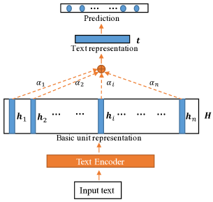
Our work leverages the attention-based self-explaining method (Lin et al., 2017), as shown in Figure 1. First, our text encoder (§3) formulates an input text into a list of basic units, learning a vector representation for each, where the basic units can be words, phrases, or arbitrary ngrams. Then, the attention mechanism is leveraged over all basic units, and sums up all unit representations based on the attention weights {}. Eventually, the attention weight will be used to reveal how important a basic unit is. The last prediction layer takes the fixed-length text representation as input, and makes the final prediction.
Baselines: We compare two types of baseline text encoders in Figure 1. (1) Lin et al. (2017) (BiLSTM), which formulates single word positions as basic units, and computes the vector for the -th word position with a BiLSTM; (2) Extension of Mullenbach et al. (2018) (CNN). The original model in Mullenbach et al. (2018) only utilizes 4-grams. Here we extend this model to take all unigrams, bigrams, and up to -grams as the basic units.
For a fair comparison, both our approach and the baselines share the same architecture, and the only difference is the text encoder used.

3 Multi-granular text encoder
We propose the multi-granular text encoder to deal with drawbacks (as mentioned in the third paragraph of Section 1) of our baselines.
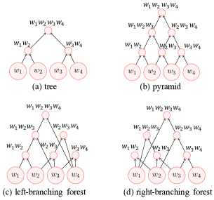
Structural basic units: We define basic units for the input text as multi-granular ngrams, organizing ngrams in four different ways. Taking a synthetic sentence as the running example, we illustrate these structures in Figure 2 (a), (b), (c) and (d), respectively. The first is a tree structure (as shown in Figure 2(a)) that includes all phrases from a (binarized) constituent tree over the input text, where no cross-boundary phrases exists. The second type (as shown in Figure 2 (b,c,d)) includes all possible ngrams from the input text, which is a superset of the tree structure. In order to reuse representations of smaller ngrams while encoding bigger ngrams, all ngrams are organized into hierarchical structures in three different ways. First, inspired by Zhao et al. (2015), a pyramid structure is created for all ngrams as shown in Figure 2(b), where leaf nodes are unigrams of the input text, and higher level nodes correspond to higher-order ngrams. A disadvantage of the pyramid structure is that some lower level nodes may be used repeatedly while encoding higher level nodes, which may improperly augment the influence of the repeated units. For example, when encoding the trigram node “”, the unigram node “” is used twice through two bigram nodes “” and “”. To tackle this issue, a left-branching forest structure is constructed for all ngrams as shown in Figure 2(c), where ngrams with the same prefix are grouped together into a left-branching binary tree, and, in this arrangement, multiple trees construct a forest. Similarly, we construct a right-branching forest as shown in Figure 2(d).
Encoding: We leverage a tree-structured LSTM composition function Tai et al. (2015); Zhu et al. (2015); Teng and Zhang (2016) to compute node embeddings for all structures in Figure 2. Formally, the state of each node is represented as a pair of one hidden vector and one memory representation , which are calculated by composing the node’s label embedding and states of its left child and right child with gated functions:
| (1) | ||||
| (2) | ||||
| (3) | ||||
| (4) | ||||
| (5) | ||||
| (6) | ||||
| (7) |
where is the sigmoid activation function, is the elementwise product, is the input gate, and are the forget gates for the left and right child respectively, and is the output gate. We set as the pre-trained word embedding for leaf nodes, and zero vectors for other nodes. The representations for all units (nodes) can be obtained by encoding each basic unit in a bottom-up order.
Comparison with baselines Our encoder is more efficient than CNN while encoding bigger ngrams, because it reuses representations of smaller ngrams. Furthermore, the same parameters are shared across all ngrams, which makes our encoder more compact, whereas the CNN baseline has to define different filters for different order of ngrams, so it requires much more parameters. Experiments show that using basic units up to 7-grams to construct the forest structure is good enough, which makes our encoder more efficient than BiLSTM. Since in our encoder, all ngrams with the same order can be computed in parallel, and the model needs at most 7 iterative steps along the depth dimension for representing a given text of arbitrary length.
4 Experiments
Dataset: We experiment on a public medical text classification dataset.111https://github.com/SnehaVM/Medical-Text-Classification Each instance consists of a medical abstract with an average length of 207 tokens, and one label out of five categories indicating which disease this document is about. We randomly split the dataset into train/dev/test sets by 8:1:1 for each category, and end up with 11,216/1,442/1,444 instances for each set.
Hyperparameters We use the 300-dimensional GloVe word vectors pre-trained from the 840B Common Crawl corpus Pennington et al. (2014), and set the hidden size as 100 for node embeddings. We apply dropout to every layer with a dropout ratio 0.2, and set the batch size as 50. We minimize the cross-entropy of the training set with the ADAM optimizer Kingma and Ba (2014), and set the learning rate is to 0.001. During training, the pre-trained word embeddings are not updated.

4.1 Properties of the multi-granular encoder
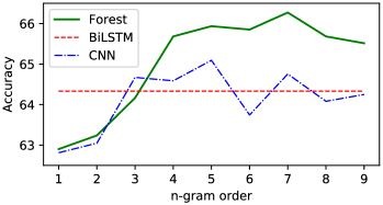
Influence of the n-gram order: For CNN and our LeftForest encoder, we vary the order of ngrams from 1 to 9, and plot results in Figure 3. For BiLSTM, we draw a horizontal line according to its performance, since the ngram order does not apply. When ngram order is less than 3, both CNN and LeftForest underperform BiLSTM. When ngram order is over 3, LeftForest outperforms both baselines. Therefore, in terms of accuracy, our multi-granular text encoder is more powerful than baselines.
| Model | Train Time | Eval Time | ACC | #Param. |
|---|---|---|---|---|
| CNN | 57.0 | 2.6 | 64.8 | 848,228 |
| BiLSTM | 92.1 | 4.6 | 64.5 | 147,928 |
| LeftForest | 30.3 | 1.4 | 66.2 | 168,228 |
Efficiency: We set ngram order as 7 for both CNN and our encoder. Table 2 shows the time cost (seconds) of one iteration over the training set and evaluation on the development set. BiLSTM is the slowest model, because it has to scan over the entire text sequentially. LeftForest is almost 2x faster than CNN, because LeftForest reuses lower-order ngrams while computing higher-order ngrams. This result reveals that our encoder is more efficient than baselines.
Model size: In Table 2, the last two columns show the accuracy and number of parameters for each model. LeftForest contains much less parameters than CNN, and it gives a better accuracy than BiLSTM with only a small amount of extra parameters. Therefore, our encoder is more compact.
4.2 Model performance
| Model | Accuracy |
|---|---|
| BiLSTM | 62.7 |
| CNN | 62.5 |
| Tree | 63.8 |
| Pyramid | 63.7 |
| LeftForest | 64.6 |
| RightForest | 64.5 |
| BiForest | 65.2 |
Table 3 lists the accuracy on the test set, where BiForest represents each ngram by concatenating representations of this ngram from both the LeftForest and the RightForest encoders. We get several interesting observations: (1) Our multi-granular text encoder outperforms both the CNN and BiLSTM baselines regardless of the structure used; (2) The LeftForest and RightForest encoders work better than the Tree encoder, which shows that representing texts with more ngrams is helpful than just using the non-overlapping phrases from a parse tree; (3) The LeftForest and RightForest encoders give better performance than the Pyramid encoder, which verifies the advantages of organizing ngrams with forest structures; (4) There is no significant difference between the LeftForest encoder and the RightForest encoder. However, by combining them, the BiForest encoder gets the best performance among all models, indicating that the LeftForest encoder and the RightForest encoder complement each other for better accuracy.

4.3 Analysis of explainability
Qualitative analysis
The following text is a snippet of an example from the dev set. We leverage our BiForest model to extract ngrams whose attention scores are higher than 0.05, and use the bold font to highlight them. We extracted three ngrams as supporting evidence for its predicted category “nervous system diseases”. Both the spontaneous extradural spinal hematoma and the spinal arteriovenous malformation are diseases related to the spinal cord, therefore they are good evidence to indicate the text is about “nervous system diseases”.
Snippet: Value of magnetic resonance imaging in spontaneous extradural spinal hematoma due to vascular malformation : case report . A case of spinal cord compression due to spontaneous extradural spinal hematoma is reported . A spinal arteriovenous malformation was suspected on the basis of magnetic resonance imaging. Early surgical exploration allowed a complete neurological recovery .
Quantitative analysis
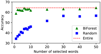
For each instance in the training set and the dev set, we utilize the attention scores from BiForest to sort all ngrams, and create different copies of the training set and development set by only keeping the first important words. We then train and evaluate a BiLSTM model with the newly created dataset. We vary the number of words among {1, 2, 3, 4, 5, 6, 7, 8, 9, 10, 20, 30, 40, 50}, and show the corresponding accuracy with the green triangles in Figure 4. We define a Random baseline by randomly selecting a sub-sequence containing words, and plot its accuracy with blue squares in Figure 4. We also take a BiLSTM model trained with the entire texts as the upper bound (the horizontal line in Figure 4). When using only a single word for representing instances, single words extracted from our BiForest model are significantly more effective than randomly picked single words. When utilizing up to five extracted words from our BiForest model for representing each instance, we can obtain an accuracy very close to the upper bound. Therefore, the extracted evidence from our BiForest model are truly effective for representing the instance and its corresponding category.
5 Conclusion
We proposed a multi-granular text encoder for self-explaining text categorization. Comparing with the existing BiLSTM and CNN baselines, our model is more accurate, efficient and compact. In addition, our model can extract effective and intuitive evidence to support its predictions.
References
- Devlin et al. (2018) Jacob Devlin, Ming-Wei Chang, Kenton Lee, and Kristina Toutanova. 2018. Bert: Pre-training of deep bidirectional transformers for language understanding. arXiv preprint arXiv:1810.04805.
- Kingma and Ba (2014) Diederik Kingma and Jimmy Ba. 2014. Adam: A method for stochastic optimization. arXiv preprint arXiv:1412.6980.
- Lei et al. (2016) Tao Lei, Regina Barzilay, and Tommi Jaakkola. 2016. Rationalizing neural predictions. arXiv preprint arXiv:1606.04155.
- Li et al. (2015) Jiwei Li, Xinlei Chen, Eduard Hovy, and Dan Jurafsky. 2015. Visualizing and understanding neural models in nlp. arXiv preprint arXiv:1506.01066.
- Lin et al. (2017) Zhouhan Lin, Minwei Feng, Cicero Nogueira dos Santos, Mo Yu, Bing Xiang, Bowen Zhou, and Yoshua Bengio. 2017. A structured self-attentive sentence embedding. arXiv preprint arXiv:1703.03130.
- Mullenbach et al. (2018) James Mullenbach, Sarah Wiegreffe, Jon Duke, Jimeng Sun, and Jacob Eisenstein. 2018. Explainable prediction of medical codes from clinical text. arXiv preprint arXiv:1802.05695.
- Pennington et al. (2014) Jeffrey Pennington, Richard Socher, and Christopher D Manning. 2014. Glove: Global vectors for word representation. In EMNLP.
- Tai et al. (2015) Kai Sheng Tai, Richard Socher, and Christopher D Manning. 2015. Improved semantic representations from tree-structured long short-term memory networks. arXiv preprint arXiv:1503.00075.
- Teng and Zhang (2016) Zhiyang Teng and Yue Zhang. 2016. Bidirectional tree-structured lstm with head lexicalization. arXiv preprint arXiv:1611.06788.
- Vaswani et al. (2017) Ashish Vaswani, Noam Shazeer, Niki Parmar, Jakob Uszkoreit, Llion Jones, Aidan N Gomez, Łukasz Kaiser, and Illia Polosukhin. 2017. Attention is all you need. In Advances in Neural Information Processing Systems, pages 6000–6010.
- Zhao et al. (2015) Han Zhao, Zhengdong Lu, and Pascal Poupart. 2015. Self-adaptive hierarchical sentence model. In IJCAI, pages 4069–4076.
- Zhu et al. (2015) Xiaodan Zhu, Parinaz Sobihani, and Hongyu Guo. 2015. Long short-term memory over recursive structures. In International Conference on Machine Learning, pages 1604–1612.