Rate Splitting with Finite Constellations: The Benefits of Interference Exploitation vs Suppression
Abstract
Rate-Splitting (RS) has been proposed recently to enhance the performance of multi-user multiple-input multiple-output (MU-MIMO) systems. In RS, a user message is split into a common and a private part, where the common part is decoded by all users, while the private part is decoded only by the intended user. In this paper, we study RS under a phase-shift keying (PSK) input alphabet for multi-user multi-antenna system and propose a constructive interference (CI) exploitation approach to further enhance the sum-rate achieved by RS under PSK signaling. To that end, new analytical expressions for the ergodic sum-rate are derived for two precoding techniques of the private messages, namely, 1) a traditional interference suppression zero-forcing (ZF) precoding approach, 2) a closed-form CI precoding approach. Our analysis is presented for perfect channel state information at the transmitter (CSIT), and is extended to imperfect CSIT knowledge. A novel power allocation strategy, specifically suited for the finite alphabet setup, is derived and shown to lead to superior performance for RS over conventional linear precoding not relying on RS (NoRS). The results in this work validate the significant sum-rate gain of RS with CI over the conventional RS with ZF and NoRS.
Index Terms:
Rate splitting, zero forcing, constructive interference, phase-shift keying signaling.I Introduction
The recent years have witnessed the widespread application of multi-user multiple-input multiple-output (MU-MIMO) systems, due to their reliability and high spectral efficiency [2, 3, 4]. However, in practical communication networks, the advantages of MU-MIMO systems are often impacted by interference [2, 3, 4]. Consequently, a considerable amount of researches has focused on improving the performance of MU-MIMO systems [4, 5, 6]. In this regard, Rate-Splitting (RS) approach was recently proposed and investigated in different scenarios to enhance the performance of MU-MIMO systems [7, 8, 9, 10, 11]. RS scheme splits the users’ messages into a common message and private messages, and superimposes the common message on top of the private messages. Using Successive Interference Cancellation (SIC) at the receivers, the common message is first decoded by all the users, and each private message is then decoded only by its intended user. By adjusting the message split and the power allocated to the common and private messages, RS has the ability to better handle the multiuser interference. RS has been studied in multiuser multi-antenna setups with both perfect and imperfect CSIT. In [9], authors analyzed the sum-rate gain achieved by RS over conventional multi-user linear precoding (NoRS) in a two-user multi-antenna broadcast channel with imperfect CSIT, and considered that the common message is transmitted via a space and space-time design. In [9, 8, 10, 11], again considering imperfect CSIT, the authors leveraged convex optimization to optimize the precoders of the common and private messages to maximize the ergodic sum-rate and the max-min rate, respectively, and again showed the superiority of RS over NoRS. In [12], RS was designed and its performance analyzed for Massive MIMO with imperfect CSIT and shown to outperform the conventional NoRS approach. In [11], a multi-pair Massive MIMO relay system with imperfect CSIT was considered and RS was shown to lead to higher robustness compared to NoRS. In [13], RS was designed for a multi-antenna multi-cell system with imperfect CSIT, and showed the superiority in a Degrees-of-Freedom sense over NoRS. The benefits of RS have also been highlighted in multiuser multi-antenna system with perfect CSIT as in [14, 15], and performance gains were highlighted over both NoRS and power-domain Non-Orthogonal Multiple Access (NOMA) techniques.
Another line of research has recently proposed constructive interference (CI) precoding techniques to enhance the performance of downlink MU-MIMO systems [16, 17, 18, 19]. In contrast to the conventional interference mitigation techniques, where the knowledge of the interference is used to cancel it, the main idea of the CI is to use the interference to improve the system performance. The CI precoding technique exploits interference that can be known to the transmitter to increase the useful signal received power [16, 17, 18, 19]. That is, with the knowledge of the CSI and users’ data symbols, the interference can be classified as constructive and destructive. The interference signal is considered to be constructive to the transmitted signal if it pushes/moves the received symbols away from the decision thresholds of the constellation towards the direction of the desired symbol. Accordingly, the transmit precoding can be designed such that the resulting interference is constructive to the desired symbol.
The concept of CI has been extensively studied in literature. This line of work has been introduced in [16], where the CI precoding scheme for the downlink of PSK-based MIMO systems has been proposed. In this work, it was shown that the effective signal to interference-plus-noise ratio (SINR) can be enhanced without the need to increase the transmitted signal power at the base station (BS). In [17], an optimization-based precoder in the form of pre-scaling has been designed for the first time using the concept of CI. Thereof, [18] proposed transmit beamforming schemes for the MU-MIMO downlink that minimize the transmit power for generic PSK signals. In [20], a transmission algorithm that exploits the constructive multiuser interference was proposed. The authors in [21, 22] studied a general category of CI regions, namely distance preserving CI region, where the full characterization for a generic constellation was provided. In [19, 23], CI precoding scheme was applied in wireless power transfer scenario in order to minimize the transmit power while guaranteeing the energy harvesting and the quality of service (QoS) constraints for PSK messages. Further work in [24] applied the CI concept to Massive MIMO systems. Very recently, the authors in [25] derived closed-form precoding expression for CI exploitation in the MU-MIMO downlink. The closed-form precoder in this work has for the first time made the application of CI exploitation practical, and has further paved the way for the development of communication theoretic analysis of the benefits of CI. While the above literature has addressed traditional downlink transmission, the application of the CI concept to RS approaches remains an open problem, due to the finite constellation input that CI requires.
Accordingly, in this paper, we provide the first attempt to combine those two lines of research on RS and CI, and employ the CI precoding technique to further enhance the sum-rate achieved by RS scheme in MU-MIMO systems under a PSK input alphabet111We note that, while traditional analysis focus on Gaussian signaling, the study of finite constellation signaling is of particular importance, since finite constellations are applied in practice.. In this regard and in order to provide fair comparison, new analytical expressions for the ergodic sum-rate are derived for two precoding techniques of the private messages, namely, 1) a closed-form CI precoding approach, 2) a traditional interference suppression zero-forcing (ZF) precoding approach. Our analysis is presented for perfect channel state information at the BS (CSIT), and extended to imperfect CSIT. Additionally, the conventional transmission, NoRS, is also studied in this paper. Furthermore, a power allocation scheme that can achieve superiority of RS over the NoRS in finite alphabet systems is proposed and investigated.
For clarity we list the major contributions of this work as follows.
-
1.
First, new analytical expressions for the ergodic sum-rate are derived for RS based on finite constellations with CI and ZF precoding schemes for the private messages. Both perfect CSIT and imperfect CSIT are considered. This contrasts with the existing literature that either study NoRS based on finite constellation with CI/ZF precoding, or RS based on Gaussian inputs. This is the first paper that a) studies RS with finite constellations, b) combines RS with CI precoding.
-
2.
Second, a novel power allocation algorithm is introduced to optimize the resulting sum-rate in the finite alphabet scenario.
-
3.
Third, Monte-Carlo simulations are provided to confirm the analysis, and the impact of the different system parameters on the achievable sum-rate are examined and investigated.
The results in this work show clearly that the sum-rate of RS with CI outperforms the sum rate of RS with ZF and NoRS (with either ZF or CI) transmission techniques.
Notations: , , and denote a scalar, a vector and a matrix, respectively. , and denote conjugate transposition, transposition and diagonal of a matrix, respectively. denotes average operation. denotes the element in , denotes the absolute value, , and denotes the second norm. represents an matrix, and denotes the identity matrix.
II System Model
We consider a MU-MIMO system, in which an antennas BS node communicates with -single antenna users in a downlink scenario using the RS strategy. In this system the channels are assumed to be independent identically distributed (i.i.d) Rayleigh fading channels. The channel matrix between the BS and the users is denoted by , which can be written as where contains i.i.d elements represent small-scale fading coefficients and is a diagonal matrix represents the path-loss attenuation with , where is the distance between the BS and the user, and is the path loss exponent. It is also assumed that the signal is equiprobably drawn from an -PSK constellation.
Therefore, the BS transmits independent messages uniformly drawn from the sets , and intended for users respectively. In RS, each user message is split into a common part and a private part, i.e., 222The subscript here denotes total, which is explained that is composed of two parts. The subscripts and are used for common part and private parts, respectively. with , , and . The common message is composed by packing the common parts such that . The resulting messages are encoded into the independent data streams , where and represent the encoded common and private symbols [8]. The symbols are grouped in a signal vector , where . Then the symbols are mapped to the BS antennas by a linear precoding matrix defined as where denotes the common precoder and is the private precoder. Therefore, the transmitted signal can be mathematically expressed by [7, 9, 8]
| (1) |
where , denotes the common precoder of the common message and is the private precoder. In addition, and are the power allocated to the common message and the power allocated to the private message, respectively, where and , and is the total power333We assume a uniform power allocation among all the private symbols, similarly to other works on RS [9, 12]. Although this assumption does not produce the optimal performance, it allows us to find tractable results. This assumption is commonly used in practice, e.g. LTE and LTE-A. . Conventional multi-user linear precoding without RS, NoRS, is a particular instance of the RS strategy and is obtained by turning of the common message and allocating all transmit power exclusively to the privates messages. The received signal at the user in this system can be written as
| (2) |
where is the channel vector from the BS to user , is the additive wight Gaussian noise (AWGN) at the user, . At the user side, the common symbol is decoded firstly by treating the interference from the private messages as noise, and then each user decodes its own message after canceling the common message using SIC technique. Therefore, after perfectly removing the contribution from the common message, the received signal at the user in this system can be written as
| (3) |
where and . The sum rate in this scenario can be expressed by
| (4) |
where is the rate for the common part, , is the rate for the common message at user , and is the rate for the private part at the user.
In this work, both perfect CSIT and imperfect CSIT are considered, and delay-tolerant transmission is assumed. Hence the channel coding can be achieved over a long sequence of channel states. Therefore, transmitting the common and the private messages at ergodic rates and , respectively, guarantees successful decoding by the user [11]. Hence, to guarantee the common message, , is successfully decoded and then canceled by the users, it should be sent at an ergodic rate not exceeding . Finally, the ergodic sum rate can be expressed by,
| (5) |
III Ergodic Sum Rate Analysis under PSK signaling and perfect CSIT
In this scenario, the BS has perfect knowledge of the CSI, and the precoding matrices have been designed based on this perfect knowledge. Therefore, in this section two precoding techniques are considered. In the first one, we use maximum ratio transmission (MRT) for the common message and CI for the private messages, and in the second one we use MRT for the common message and ZF for the private messages.
III-A RS: MRT/CI
In this scenario MRT technique is used for common message and CI precoding for the private messages. Therefore, the precoder for the common and the private messages can be written, respectively, as [12, 25]
| (6) |
| (7) |
where and are the scaling factor to meet the transmit power constraint at the transmitter, while and . For simplicity and mathematical tractability but without loss of generality, the normalization constants and are designed to ensure that the long-term total transmit power at the source is constrained, so it can be written as [6, 25] and . Since and has Gamma and Wishart distributions respectively, we can find that, and , where and [26].
From (5), we now need to calculate the ergodic rate for the common and private messages as follows.
III-A1 Ergodic Rate for the Common Part
| (8) |
where , , and contain symbols, which are taken from the equiprobable constellation set with cardinality 444Each input consists of symbols taken from the -PSK constellation..
Proof:
The proof of the above follows known derivations from the finite constellation rate analysis literature, and due to the paper length limitation, the proof of (8) has been omitted in this paper. ∎
Similar to the Gaussian input assumption case, (8) reveals that the achievable rate suffering from the interference caused by other signals. The first term in (8), , contains all the received signals at user , while the second term, , contains only the interference signals.
By invoking Jensen inequality, the first term in (8), , can be expressed by
| (9) |
Since the noise, , has Gaussian distribution, the average over the noise can be derived as
| (10) |
Using the integrals of exponential function in [30], we can find
| (11) |
Now, the average over the channel can be derived as
| (12) |
which can be written as
| (13) |
where is a vector all the elements of this vector are zeros except the element is one. Therefore, the first term can be expressed as
| (14) |
where , . Now, we can simplify the last expression in (14) to
| (15) |
The term in (14) can be reduced to Let which has Gamma distribution, .i.e., , with degrees of freedom, therefore the average over is the moment generating function (MGF) of the term, which can be found easily as
| (16) |
For the second term, , similarly using Jensen inequality we can write
| (17) |
Similarly as in (10), since has Gaussian distribution, we can write as
| (18) |
| (19) |
where . Therefore we can get,
| (20) |
which can be obtained as
| (21) |
where is the Hypergeometric function.
It is noted that Jensen’s inequality has been used in the two terms in (8). Accordingly, the resulting expression cannot lead to a strict bound on the resulting rate. Nevertheless, since the involved rate is based on a finite constellation, the resulting low-SNR and high-SNR approximation match the exact rate. In the intermediate SNR regions, it can be observed that the bounding errors of the two terms have similar values which results in an accurate overall approximation, as already verified in relevant analysis in [28]. We note that the rate approximations show a very close match to our Monte Carlo simulations in our results of Section VII.
III-A2 Ergodic Rate for the Private Part
The ergodic rate for the private part at user under PSK signaling, using CI precoding technique can be written as[27, 28, 29],
| (22) |
III-B RS: MRT/ZF
In this case we implement MRT technique for common signal and ZF precoding for the private messages. Therefore, the precoding for the common and the private messages can be written, respectively, as [12, 25]
| (23) |
| (24) |
where and are the scaling factors to meet the transmit power constraint at the transmitter, which can be expressed as and . Similarly as in the MRT/CI scenario, and for mathematical tractability but without loss of generality, the normalization constants and are designed to ensure that the long-term total transmit power at the source is constrained, so it can be written as [6, 25], and , respectively. Since and both have Gamma distribution [5, 16], we can find that, and [26].
III-B1 Ergodic Rate for the Common Part
The ergodic rate for the common part at user k can be written as
| (25) |
where . By using Jensen inequality, the first term in (25), , can be written as
| (26) |
Since the noise is Gaussian distributed, using the integrals of exponential function in [30] the average over the noise can be derived as
| (27) |
Now, we can write as
| (28) |
Since the term has Gamma distribution, .i.e., , the average can be derived as
| (29) |
Applying Gaussian Quadrature rule, the average can be obtained by,
| (30) |
where and are the zero and the weighting factor of the Laguerre polynomials, respectively [31]. Similarly, for the second term , using Jensen inequality we can write,
| (31) |
The average over the noise can be obtained as
| (32) |
III-B2 Ergodic Rate for the Private Part
The ergodic rate for the private message at the user, under PSK signaling using ZF precoding technique can be written as[27, 28, 29],
| (33) |
III-C Conventional Transmission Without Rate Splitting (NoRS)
The ergodic rate at the user in conventional transmission without RS is expressed by
| (34) |
In CI case, the precoding matrix is given in (7), and the expectation in (34) can be derived using Jensen inequality as in (21). On the other hand, in ZF scenario the precoding matrix is given in (24), and then the expectation in (34) can be derived using Jensen inequality as in (32).
Please note that, in case the users’ locations are randomly distributed, the ergodic sum-rate with respect to each user location can be calculated easily by averaging the derived sum-rate expression over all possible user locations.
IV Ergodic Sum Rate Analysis under PSK signaling and Imperfect CSI
In practice, the BS can estimate the channel matrix H by transmitting pilot signals. Therefore, the current channels in terms of the estimated channels, and the estimation error can be written as [32, 10], , where is the estimated channel matrix, E is the estimation error matrix. The two matrices , and E are assumed to be mutually independent and distributed as and , where is a diagonal matrix with and [32, 10], while and , is number of symbols used for channel training and is the transmit power for each pilot symbol. Consequently, the received signal can be written now as,
| (35) |
IV-A RS: MRT/CI
In this scenario, the precoder for the common and the private messages based on the estimated channels can be written, respectively, as [12, 25]
| (36) |
| (37) |
The received signal at user can be now written as
| (38) |
IV-A1 Ergodic Rate for the Common Part
The ergodic rate for the common part at user under PSK signaling in imperfect CSIT scenario, can be written as[27, 28, 29]
| (39) |
As one can see from (39), the ergodic rate is hard to further simplify, since the expectations involve several random variables. However, an approximation based on large number of antennas at the BS can be derived.
Analysis for Large
In this case we analyze the ergodic rate when the number of BS antennas is large , driven by the increasing research interest in MU-MIMO systems with a large number of BS antennas.
Lemma 1.
Let and be independent vectors contain i.i.d entries with zero-mean and variances and . Therefore, following the law of large numbers, we can get [32]
| (40) |
| (41) |
where and denote almost-sure and distribution convergence, respectively.
It is well known that by deploying very large number of antennas at the BS, the small-scale fading can be averaged out. Therefore, we now can elaborate more on analyzing the impact of large-scale fading on the system performance. Using the facts in Lemma 1, (39) becomes
| (42) |
and
| (43) |
By invoking Jensen inequality, the first term in (43), , can be expressed by
| (44) |
Since the noise has Gaussian distribution, using the integrals of exponential function, we can find [30]
| (45) |
Now, the average over the user location can be derived as
| (46) |
For analytical convenience, in this section we assume that the cell shape is approximated by a circle of radius , and the users are uniformly distributed in the cell [33]. Hence, the PDF of the users at radius relative to the BS is [33] , where is the closest distance between a user and the BS. Therefore, we can find the average over using Gaussian Quadrature rules as,
| (47) |
| (48) |
where and and are the zero and the weighting factors of the Laguerre polynomials, respectively [31].
For the second term, , similarly using Jensen inequality we can write
| (49) |
Since has Gaussian distribution, we can get
| (50) |
| (51) |
| (52) |
IV-A2 Ergodic Rate for the Private Part
The ergodic rate for the private part at user under PSK signaling, using CI precoding technique can be written as[27, 28, 29],
| (53) |
IV-B RS: MRT/ZF
In this case the precoding for the common and the private messages based on the estimated channels can be written, respectively, as
| (54) |
| (55) |
Therefore, the received signal is given by
| (56) |
IV-B1 Ergodic Rate for the Common Part
The ergodic rate for the common part at user under PSK signaling in imperfect CSI scenario can be written as[27, 28, 29],
| (57) |
For the sake of comparison, here we derive an approximation of the user rate based on a large number of antennas.
Analysis for Large
The rate for the common part at user when can be written as
| (58) |
By using Jensen inequality, the first term in (58), , can be expressed by
| (59) |
Since the noise has Gaussian distribution, the average over the noise using the integrals of exponential function can be derived as [30]
| (60) |
Now, we can write as
| (61) |
Similarly to the CI scenario, we assume that the cell shape is approximated by a circle of radius and the users are uniformly distributed in the cell [33]. Therefore, we can find the average over by
| (62) |
which can be found using Gaussian Quadrature rules as
| (63) |
For the second term , using Jensen inequality we can write
| (64) |
Since the noise has Gaussian distribution, the average can be derived as
| (65) |
IV-B2 Ergodic Rate for the Private Part
The ergodic rate for the private message at the user, under PSK signaling using ZF precoding technique can be written as[27, 28, 29]
| (66) |
By using Jensen inequality, and following similar steps as in the previous section, we can find the average of as in (65).
IV-C Conventional Transmission NoRS
The rate at the user in conventional transmission without RS is expressed by
| (67) |
For sake of comparison with using RS technique in this scenario, we study approximation of the ergodic user rate based on large number of antennas. In CI case the precoding matrix is given in (37), and the expectation in (67) can be derived using Jensen inequality as in (50) and (52). On the other hand, in ZF scenario the precoding matrix is given in (55), and then the expectation in (67) can be derived using Jensen inequality as in (65).
V Rate Maximization through RS Power Allocation
In this section, we formulate a power allocation problem for maximizing the ergodic sum-rate of the RS transmission schemes described in the previous sections. The optimal value of can be obtained by solving the following problem
| (68) |
It is worth noting that the availability of perfect CSIT enables the BS to maximize the instantaneous sum-rate by adapting the power split among the common and private messages based on the channel status. Consequently, following [11], the maximization in (68) can be moved inside the expectation and the optimum solution can be found for each channel state. In case the BS has imperfect CSIT, the BS can not evaluate the instantaneous rates, but it can access the average rates which are the expected rates for a given channel estimate. Hence, maximizing the ergodic sum-rate under imperfect CSIT can be achieved for each estimated channel [11]. For simplicity and to gain some insight, we consider ergodic sum-rate maximization problem in the two scenarios.
On one hand, the analytical optimization for the case of finite constellation signaling using the derived formulas above becomes intractable. On the other hand, the optimal can be obtained by a simple one dimensional search over . Hence, the optimal can be found by using line search methods such as golden section technique. The overall steps of golden section method to obtain the optimal is stated in Algorithm 1 [34].
Moreover, in order to reduce the complexity, two sub-optimal solutions can be considered in finite alphabet scenarios, as follows.
-
•
In the first solution, we allocate a fraction of the total power for the private messages to achieve the same sum-rate as the conventional techniques with full power. Then, the remaining power can be allocated for the common message, as considered in [12]. The sum-rate payoff of the RS scheme over the NoRS can be determined by,
| (69) |
Consequently, the ratio that achieves the superiority can be obtained by satisfying the equality, .
-
•
In the second solution, since the achievable data rate in the finite alphabet systems saturates at maximum predefined value , here at high SNR the optimal value of is the value that achieves the maximum rate with less transmit power , as in the following expression
| (70) |
Therefore, the optimum value of at high SNR is the value that satisfies (70) with minimum power .
VI Numerical Results
In this section, we present numerical results of the analytical expressions derived in this work. Monte-Carlo simulations are conducted where the channel coefficients are randomly generated. The path loss exponent is chosen to be , and assuming the users have same noise power, , and the total transmission power is , the transmit signal to noise ratio (SNR) is defined as SNR = .

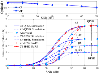
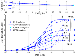
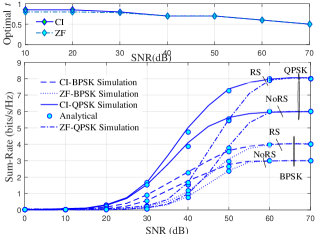
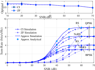
Firstly, in Fig. 1 and Fig. 2, we illustrate the sum-rate for the RS and NoRS using MRT-CI and MRT-ZF in perfect CSIT scenario and imperfect CSIT scenario, respectively, subject to BPSK and QPSK when , and . Fig. 1a and Fig. 2a present the sum-rate in the two scenarios when the distances between the BS and the users are normalized to unit value, .i.e, without the impact of the path-loss. Fig. 1b and Fig. 2b show the sum-rate when the users are uniformly distributed inside a circle area with a radius of 40m and the BS is located at the center of this area. The good agreement between the analytical and simulated results confirms the validity of the analysis introduced in this paper. Several observations can be extracted from these figures. Firstly, it is clear that the sum rate saturates at a certain SNR value, owing to the finite constellation. Secondly, the RS scheme enhances the sum-rate of the considered system and tackles the sum-rate saturation occurred in the communication systems with PSK signaling. In addition, it is evident that the CI precoding techniques outperforms the ZF technique in the all considered scenarios for a wide SNR range with an up to 10dB gain in the SNR for a given sum rate. Additionally, in Fig 1 we plot the sum-rate using 8PSK with NoRS, and observe that the sum-rate in this case saturates at the same rate as QPSK with RS, .i.e., 6 bits/s/Hz. However, at low SNR, the gain attained using QPSK with RS is higher than that using 8PSK with NoRS in all considered schemes. Comparing the results in Fig. 1a and Fig. 2a with that in Fig. 1b and Fig. 2b, one can notice that, in general, increasing the distance always degrades the achievable sum rates. In addition, when the distance between the BS and the users increases the rate saturation occurs at high SNR values, due to larger path-loss. It is also clear that, the superiority of RS with CI over RS with ZF and NoRS does not depend on the users’ locations. Furthermore, as anticipated the system performance degrade notably in the imperfect CSIT scenario. In addition, we can observe that when the number of BS antennas is high , the ZF achieves the same performance as the CI; ZF precoding can be considered as a special case of the CI precoding technique [25].
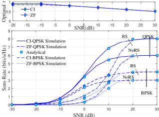

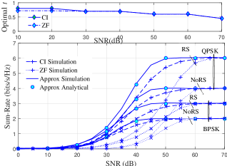
Moreover, we investigate the impact of the number of BS antennas and the number of users on the system performance. Therefore, in Fig. 3 and Fig. 4 we plot the sum-rate versus the SNR for the considered transmission schemes with BPSK, and QPSK, when , and . Fig. 3a and Fig. 4a present the sum-rate when the distances are normalized to unit value. Fig. 3b and Fig. 4b show the sum-rate when the users are uniformly distributed in a circle area of 40m radius, where the BS is located at the center of this area. From the results, it is clear that increasing the number of users and/or the number of antennas results in enhancing the achievable sum-rate in all the considered scenarios. In addition, comparing the sum rate achieved in Fig. 3a and Fig. 3b, we can see similar observations as in the case when .
Generally, from the results presented in the figures, the optimal value of the power fraction at low SNR is approximately , which means that splitting the messages and transmitting a common message is not beneficial in this SNR range. In this case only the private messages are transmitted and the RS degenerates to NoRS. This is because the users are experienced similar SNR. If there is a notable disparity of channel strengths among users, this conclusion may not hold [15]. On the other hand at high SNR the optimal value of is less than one, , which indicates that the common message is transmitted with the remaining power beyond the saturation of the private message transmission.

In order to clearly illustrate the impact of the power fraction on the system performance, we plot in Fig. 5 the sum-rate versus SNR for various values of with the CI precoding under QPSK, when m and m. Interestingly enough, it is noted that at low SNR values, , the sum-rate degrades as becomes small, and the optimal in this range is approximately close to 1. In addition, at high SNR values, , the sum-rate degrades as the value of increases, till the sum-rate reaches the achievable rate in case NoRS when .
VII Conclusions
In this paper we employed the CI precoding technique to enhance the sum-rate performed by RS scheme in MU-MIMO systems under PSK input alphabet. New analytical expressions for the ergodic sum-rate have been derived for CI precoding technique and ZF precoding technique in RS and NoRS scenarios. Furthermore, a power allocation scheme that achieves superiority of RS over NoRS in the presence of finite constellation was proposed. The results presented in this work demonstrated that RS with CI has greater sum-rate than RS with ZF and NoRS transmission techniques. In addition, increasing the number of BS antennas and/ or the number of users enhances the achievable sum-rate.
References
- [1] A. Salem and C. Masouros, “Rate splitting approach under psk signaling using constructive interference precoding technique,” in Proc. IEEE Wireless Commun. Netw. Conf. (WCNC), 2019.
- [2] M. S. John G. Proakis, Digital Communications, Fifth Edition. McGraw-Hill, NY USA, 2008.
- [3] C. B. P. Howard Huang and S. Venkatesan, MIMO Communication for cellular Networks. Springer, 2012, 2008.
- [4] Y. Wu, C. Xiao, X. Gao, J. D. Matyjas, and Z. Ding, “Linear precoder design for mimo interference channels with finite-alphabet signaling,” IEEE Transactions on Communications, vol. 61, no. 9, pp. 3766–3780, September 2013.
- [5] D. Lee, “Performance analysis of zero-forcing-precoded scheduling system with adaptive modulation for multiuser-multiple input multiple output transmission,” IET Communications, vol. 9, no. 16, pp. 2007–2012, 2015.
- [6] A. Salem and K. A. Hamdi, “Wireless power transfer in multi-pair two-way af relaying networks,” IEEE Transactions on Communications, vol. 64, no. 11, pp. 4578–4591, Nov 2016.
- [7] B. Clerckx, H. Joudeh, C. Hao, M. Dai, and B. Rassouli, “Rate splitting for mimo wireless networks: a promising phy-layer strategy for lte evolution,” IEEE Communications Magazine, vol. 54, no. 5, pp. 98–105, May 2016.
- [8] H. Joudeh and B. Clerckx, “Robust transmission in downlink multiuser miso systems: A rate-splitting approach,” IEEE Transactions on Signal Processing, vol. 64, no. 23, pp. 6227–6242, Dec 2016.
- [9] C. Hao, Y. Wu, and B. Clerckx, “Rate analysis of two-receiver miso broadcast channel with finite rate feedback: A rate-splitting approach,” IEEE Transactions on Communications, vol. 63, no. 9, pp. 3232–3246, Sept 2015.
- [10] A. Papazafeiropoulos and T. Ratnarajah, “Rate-splitting robustness in multi-pair massive mimo relay systems,” IEEE Transactions on Wireless Communications, vol. 17, no. 8, pp. 5623–5636, Aug 2018.
- [11] H. Joudeh and B. Clerckx, “Sum-rate maximization for linearly precoded downlink multiuser miso systems with partial csit: A rate-splitting approach,” IEEE Transactions on Communications, vol. 64, no. 11, pp. 4847–4861, Nov 2016.
- [12] M. Dai, B. Clerckx, D. Gesbert, and G. Caire, “A rate splitting strategy for massive mimo with imperfect csit,” IEEE Transactions on Wireless Communications, vol. 15, no. 7, pp. 4611–4624, July 2016.
- [13] C. Hao and B. Clerckx, “Miso networks with imperfect csit: A topological rate-splitting approach,” IEEE Transactions on Communications, vol. 65, no. 5, pp. 2164–2179, May 2017.
- [14] H. Joudeh and B. Clerckx, “Rate-splitting for max-min fair multigroup multicast beamforming in overloaded systems,” IEEE Transactions on Wireless Communications, vol. 16, no. 11, pp. 7276–7289, Nov 2017.
- [15] Y. Mao, B. Clerckx, and V. O. Li, “Rate-splitting multiple access for downlink communication systems: bridging, generalizing, and outperforming sdma and noma,” EURASIP Journal on Wireless Communications and Networking, vol. 2018, no. 1, p. 133, May 2018. [Online]. Available: https://doi.org/10.1186/s13638-018-1104-7
- [16] C. Masouros and E. Alsusa, “Dynamic linear precoding for the exploitation of known interference in mimo broadcast systems,” IEEE Transactions on Wireless Communications, vol. 8, no. 3, pp. 1396–1404, March 2009.
- [17] C. Masouros, M. Sellathurai, and T. Ratnarajah, “Vector perturbation based on symbol scaling for limited feedback miso downlinks,” IEEE Transactions on Signal Processing, vol. 62, no. 3, pp. 562–571, Feb 2014.
- [18] C. Masouros and G. Zheng, “Exploiting known interference as green signal power for downlink beamforming optimization,” IEEE Transactions on Signal Processing, vol. 63, no. 14, pp. 3628–3640, July 2015.
- [19] S. Timotheou, G. Zheng, C. Masouros, and I. Krikidis, “Exploiting constructive interference for simultaneous wireless information and power transfer in multiuser downlink systems,” IEEE Journal on Selected Areas in Communications, vol. 34, no. 5, pp. 1772–1784, May 2016.
- [20] M. Alodeh, S. Chatzinotas, and B. Ottersten, “Constructive multiuser interference in symbol level precoding for the miso downlink channel,” IEEE Transactions on Signal Processing, vol. 63, no. 9, pp. 2239–2252, May 2015.
- [21] A. Haqiqatnejad, F. Kayhan, and B. Ottersten, “Symbol-level precoding design based on distance preserving constructive interference regions,” IEEE Transactions on Signal Processing, vol. 66, no. 22, pp. 5817–5832, Nov 2018.
- [22] ——, “Constructive interference for generic constellations,” IEEE Signal Processing Letters, vol. 25, no. 4, pp. 586–590, April 2018.
- [23] M. R. A. Khandaker, C. Masouros, and K. K. Wong, “Constructive interference based secure precoding: A new dimension in physical layer security,” IEEE Transactions on Information Forensics and Security, vol. 13, no. 9, pp. 2256–2268, Sept 2018.
- [24] P. V. Amadori and C. Masouros, “Large scale antenna selection and precoding for interference exploitation,” IEEE Transactions on Communications, vol. 65, no. 10, pp. 4529–4542, Oct 2017.
- [25] A. Li and C. Masouros, “Interference exploitation precoding made practical: Optimal closed-form solutions for psk modulations,” IEEE Transactions on Wireless Communications, pp. 1–1, 2018.
- [26] R. J. Muirhead, Aspects of Multivariate Statistical Theory, 1982.
- [27] W. Wu, K. Wang, W. Zeng, Z. Ding, and C. Xiao, “Cooperative multi-cell mimo downlink precoding with finite-alphabet inputs,” IEEE Transactions on Communications, vol. 63, no. 3, pp. 766–779, March 2015.
- [28] Y. Wu, C. Xiao, X. Gao, J. D. Matyjas, and Z. Ding, “Linear precoder design for mimo interference channels with finite-alphabet signaling,” IEEE Transactions on Communications, vol. 61, no. 9, pp. 3766–3780, September 2013.
- [29] Y. Wu, M. Wang, C. Xiao, Z. Ding, and X. Gao, “Linear precoding for mimo broadcast channels with finite-alphabet constraints,” IEEE Transactions on Wireless Communications, vol. 11, no. 8, pp. 2906–2920, August 2012.
- [30] M. Abramowitz and I. A. Stegun, Handbook of Mathematical Functions With Formulas, Graphs, and Mathematical Tabl, Washington,D.C.: U.S. Dept. Commerce, 1972.
- [31] ——, Handbook of Mathematical Functions With Formulas, Graphs, and Mathematical Tabl, Washington,D.C.: U.S. Dept. Commerce, 1972.
- [32] H. Q. Ngo, E. G. Larsson, and T. L. Marzetta, “Energy and spectral efficiency of very large multiuser mimo systems,” IEEE Transactions on Communications, vol. 61, no. 4, pp. 1436–1449, April 2013.
- [33] M. . Alouini and A. J. Goldsmith, “Area spectral efficiency of cellular mobile radio systems,” IEEE Transactions on Vehicular Technology, vol. 48, no. 4, pp. 1047–1066, July 1999.
- [34] J. Kim, H. Lee, C. Song, T. Oh, and I. Lee, “Sum throughput maximization for multi-user mimo cognitive wireless powered communication networks,” IEEE Transactions on Wireless Communications, vol. 16, no. 2, pp. 913–923, Feb 2017.