An Approach to Efficient Fitting of Univariate and Multivariate Stochastic Volatility Models

Abstract

The stochastic volatility model is a popular tool for modeling the volatility of assets. The model is a nonlinear and non-Gaussian state space model, and consequently is difficult to fit. Many approaches, both classical and Bayesian, have been developed that rely on numerically intensive techniques such as quasi-maximum likelihood estimation and Markov chain Monte Carlo (MCMC). Convergence and mixing problems still plague MCMC algorithms when drawing samples sequentially from the posterior distributions. While particle Gibbs methods have been successful when applied to nonlinear or non-Gaussian state space models in general, slow convergence still haunts the technique when applied specifically to stochastic volatility models. We present an approach that couples particle Gibbs with ancestral sampling and joint parameter sampling that ameliorates the slow convergence and mixing problems when fitting both univariate and multivariate stochastic volatility models. We demonstrate the enhanced method on various numerical examples.

Keywords: Stochastic Volatility, Particle Gibbs, Particle Filter, Ancestral Sampling, Efficient Markov Chain Monte Carlo.

1 The Problem

Most models of volatility that are used in practice are of a multiplicative form, modeling the return of an asset, say $y_{t}$, observed at discrete time points, $t=1,\dots,n$, as

$$y_{t}=\sigma_{t}\epsilon_{t}$$ (1)

where $\epsilon_{t}$ is an iid sequence and the volatility process $\sigma_{t}$ is a non-negative stochastic process such that $\epsilon_{t}$ is independent of ${\sigma}_{s}$ for all $s\leq t$. It is often assumed that ${\epsilon}_{t}$ has zero mean and unit variance.

The basic univariate discrete-time stochastic volatility (SV) model writes the returns and the stationary log volatility, $x_{t}=\log{\sigma}_{t}^{2}$, as

$$x_{t} =\mu+\phi(x_{t-1}-\mu)+\sigma w_{t}$$ (2)

$$y_{t} =\beta\exp\bigl{\{}{\tfrac{1}{2}}x_{t}\bigr{\}}\epsilon_{t},$$ (3)

where $x_{0}\sim\operatorname{N}(\mu,\frac{\sigma^{2}}{1-\phi^{2}})$, $w_{t}\stackrel{{\scriptstyle\mathrm{iid}}}{{\sim\,}}\operatorname{N}(0,1)$, and $\epsilon_{t}\stackrel{{\scriptstyle\mathrm{iid}}}{{\sim\,}}\operatorname{N}(0,1)$ are all independent processes. The volatility process $x_{t}$ is not observed directly, but only through the observations, $y_{t}$. The constant $\mu$ is sometimes called a leverage effect and hence the model is also called the SV model with leverage when $\mu\neq 0$. The detailed econometric properties of the model are discussed in Shephard, (1996) and Taylor, (1994, 2008).

The model (2)–(3) is a nonlinear state space model, and Bayesian analysis of such models can be approached via particle Gibbs methods; e.g., Douc et al., (2014, Chap. 12). Early MCMC approaches to the problem may be found in Carlin et al., (1992), Kim et al., (1998), Jacquier et al., (1994), and Taylor, (1994).

Let $\Theta=(\mu,\beta,\phi,\sigma)$ represent the parameters, denote the observations as $y_{1:n}=\{y_{1},\dots,y_{n}\}$, and the states (log-volatility) by $x_{0:n}=\{x_{0},x_{1},\dots,x_{n}\}$, with $x_{0}$ being the initial state. To run a full Gibbs sampler, we alternate between sampling model parameters and latent state sequences from their respective full conditional distributions. Letting $\operatorname{p}(\cdot)$ denote a generic density, we have the following:

Procedure 1 (Generic Gibbs Sampler for State Space Models).

1. Draw $\Theta^{\prime}\sim\operatorname{p}(\Theta\mid x_{0:n},y_{1:n})$

2. Draw $x_{0:n}^{\prime}\sim\operatorname{p}(x_{0:n}\mid\Theta^{\prime},y_{1:n})$

Procedure 1-(i) is generally much easier because it conditions on the complete data $\{x_{0:n},y_{1:n}\}$. Procedure 1-(ii) amounts to sampling from the joint smoothing distribution of the latent state sequence and is generally difficult. For linear Gaussian models, however, both parts of Procedure 1 are relatively easy to perform (Frühwirth-Schnatter,, 1994; Carter and Kohn,, 1994; Shumway and Stoffer,, 2017, Chap. 6).

For nonlinear models, Procedure 1-(ii) can be performed using particle methods. Del Moral, (1996) introduced the particle filter to sample the hidden states together from the conditional distribution. However, particle filtering suffered from the path degeneracy, which makes sampling unreliable for long time series as mentioned in Doucet et al., (2000). To avoid path degeneracy, several resampling methods were introduced in late 1990s (e.g., Doucet et al.,, 2000; Liu and Chen,, 1998). While the Forward Filter Backward Simulator (FFBSi) and the Forward Filter Backward Smoother (FFBSm) were introduced in Doucet et al., (2000) and Godsill et al., (2004) to handle path degeneracy, the techniques required the generation of many particles and resulted in an approximation to the desired posterior distribution rather than yielding draws from the posterior distribution of interest.

Andrieu et al., (2010) introduced the particle Markov chain Monte Carlo (PMCMC) method, which proposed a conditional particle filter (CPF) to ease the difficulty of performing Procedure 1-(ii). The CPF is invariant in the sense that the kernel leaves $\operatorname{p}(x_{0:n}\mid\Theta^{\prime},y_{1:n})$ invariant; that is, all elements of the chain have the target distribution. CPF, however, suffers from the path degeneracy and works well only for short time series; otherwise, it is necessary to generate an extremely large number of particles. One way to solve this problem involved a backward simulation sweep (Whiteley et al.,, 2010). However, the method is also computationally expensive. On the other hand, Lindsten et al., (2014) introduced a CPF with ancestral sampling (CPF-AS). The addition of ancestral sampling improved on the problem path degeneracy while being robust to the number of particles generated. In fact, the method works very well with a small number of particles and consequently is an invariant and efficient particle filter.

The benefits of using CPF-AS to overcome the difficulty of performing Procedure 1-(ii) is demonstrated using a number of examples in Lindsten et al., (2014) and in Douc et al., (2014, Chap. 12), where Procedure 1 is called Particle Gibbs with Ancestor Sampling (PGAS) when CPF-AS is used for step Procedure 1-(ii).

As previously stated, step Procedure 1-(i) is typically the easier step. Usually, one puts normal priors on the leverage and (or beta priors) on the regression parameter(s), and inverse gamma priors on the scale parameters. That is, current methods proceed as if $\phi$ is a regression parameter and $\sigma$ is a scale parameter and this treatment is what leads to the inefficiency for this particular model. The problem for SV models is that $\phi$ behaves like a scale parameter as well as a regression parameter. For example, the autocorrelation function (ACF) of $\{y_{t}^{2}\}$ is given by

$$\operatorname{Cor}(y^{2}_{t},y^{2}_{t+h})=\frac{\exp(\sigma_{x}^{2}\phi^{h})-1}{\kappa_{\epsilon}\exp(\sigma_{x}^{2})-1}\,,\quad h=1,2,\dots\,,$$ (4)

where $\kappa_{\epsilon}$ is the kurtosis of the noise, ${\epsilon}_{t}$ and $\sigma_{x}^{2}=\sigma^{2}/(1-\phi^{2})$. For SV models, the ACF values are small and the decay rate as a function of lag is less than exponential and somewhat linear. This means that if you specify values for $\phi$ but allow us to control $\sigma$ (and consequently $\sigma_{x}$), we can make the model ACF to look approximately the same no matter which values of $\phi$ are chosen. This is accomplished by moving $\phi$ and $\sigma$ in opposite directions. Another way of looking at the problem is to let (with $\mu=0$ and $\beta=1$) $\xi_{t}=\frac{1}{2\sigma_{x}}x_{t}$ and $\zeta_{t}={\tfrac{1}{2}}w_{t}$ so we may write (3) as

$$y_{t}=\operatorname{e}^{\sigma_{x}\phi\xi_{t-1}}\operatorname{e}^{\sigma\cdot\zeta_{t}}\epsilon_{t}\,,$$ (5)

noting that $\xi_{t-1}$ and $\zeta_{t}$ are independent stationary ${\tfrac{1}{2}}\operatorname{N}(0,1)$s. It is clear from (5) that $\sigma$ and $\phi$ are scale parameters of the $\xi_{t}$ process and $\sigma$ is a scale parameter of the $\zeta_{t}$ noise process; we see that we can keep the scale of the data approximately the same by moving $\phi$ and $\sigma$ in opposite directions.

Figure 1: top: Two data sequences (A and B) of length 1000 generated from different two-parameter SV models, I: $\phi=.92$, $\sigma=1.5$ and II: $\phi=.97$, $\sigma=1$. bottom: The ACF of each generated series squared (A and B) and the theoretical ACFs of SV models I and II as lines. The model (I or II) generating each series (A or B) is identified in the text.

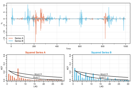
For example, Figure 1 shows two data sequences (A and B) of length 1000 generated from two different SV models, (2)–(3), with ($\mu=0$, $\beta=.1$) Model I: $\phi=.92$, $\sigma=1.5$, and Model II: $\phi=.97$, $\sigma=1$. The ACF of each generated series squared (A and B) and the theoretical ACFs of SV models I and II as lines. While the AR parameter, $\phi$, is very different in each model, the simulated series look very much the same. In fact, counterintuitively, series A corresponds to Model II: $\phi=.97$, $\sigma=1$, and series B corresponds to Model I: $\phi=.92$, $\sigma=1.5$.

While CPF-AS can improve the mixing of the sampler for SV models, there are problems with slow convergence as noted by several authors (e.g., Chib and Greenberg,, 1996; Kim et al.,, 1998) because of the relationship between the parameters as previously noted. The problem persists to this day as one can see in the vignettes of the R package stochvol (Kastner and Hosszejni,, 2019). The inefficiency of the sampler is due to the fact that (in the two-parameter model) Procedure 1-(i) is typically carried out in two steps by drawing from the univariate posteriors $\operatorname{p}(\phi\mid\sigma,x_{0:n},y_{1:n})$ and $\operatorname{p}(\sigma\mid\phi,x_{0:n},y_{1:n})$.

As an example, we performed particle Gibbs with ancestral sampling (PGAS) on Series B ($n=1000$) shown in Figure 1, which was generated from Model I,

$$x_{t}=.92x_{t-1}+1.5w_{t}\quad\text{and}\quad y_{t}=.1\exp\bigl{\{}{\tfrac{1}{2}}x_{t}\bigr{\}}\epsilon_{t}\,.$$

For Procedure 1-(i) we used normal and inverse gamma priors for $\phi$ and $\sigma^{2}$, respectively. That is, with prior $\sigma^{2}\sim{\rm IG}(a_{0}/2,b_{0}/2)$, where IG denotes the inverse (reciprocal) gamma distribution,

$$\sigma^{2}\mid\phi,x_{0:n},y_{1:n}\sim{\rm IG}\Bigl{(}\tfrac{1}{2}(a_{0}+n+1),\ \tfrac{1}{2}\bigl{\{}{b_{0}}+\sum_{t=1}^{n}[x_{t}-\phi x_{t-1}]^{2}\bigr{\}}\Bigr{)}\,.$$ (6)

With prior $\phi\sim\operatorname{N}(\mu_{\phi},\sigma_{\phi}^{2})$, we have $(\phi\mid\sigma,x_{0:n},y_{1:n})\sim\operatorname{N}(Bb,B)$, where

$$B^{-1}=\frac{1}{\sigma^{2}_{\phi}}+\frac{1}{\sigma^{2}}\sum_{t=1}^{n}{x_{t-1}^{2}}\,,\qquad b=\frac{\mu_{\phi}}{\sigma^{2}_{\phi}}+\frac{1}{\sigma^{2}}\sum_{t=1}^{n}x_{t}x_{t-1}\,.$$ (7)

For the sake of exposition, we held $\mu$ and $\beta$ fixed at their given values of $0$ and $.1$, respectively. In addition, the values for $\sigma$ are larger than is typical for actual data, but the large values help emphasize the problem.

For Procedure 1-(ii), we used CPF-AS (Procedure 4) with $N=20$ particles; details are given in the next section. This example is similar to the experiment discussed in Lindsten et al., (2013, Sec. 7.1), however we use simulated data so that we know the model is correct (and does not add to convergence problem considerations).

Figure 2: Particle Gibbs with individual parameter sampling on Series B shown in Figure 1. The actual parameters are $\phi=.92$ and $\sigma=1.5$. top: Separate draws of $\phi$ and $\sigma$ in order along with a lowess smooth to emphasize the cyclic behavior of the draws. bottom: The sample ACF of the traces (left), and a scatterplot (right) of the pairs of values in each draw with the posterior means of $.978$ and $1.303$ highlighted.

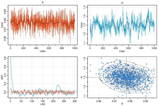
Figure 2 shows the results of the experiment. The top row shows the draws of $\phi$ and $\sigma$ in order, the bottom left shows the sample ACF of the traces, and on the right there is a scatterplot of the pairs of values in each draw. One sees the slow convergence problem reported in Chib and Greenberg, (1996) and Kim et al., (1998). The sampling procedure with CPF-AS ameliorates the slow convergence problem to some degree, but is not a remedy because of relationship between the parameters seen in the scatterplot and previously discussed leads to a type of meandering through the sample spaces of the parameters. In fact, the sample paths look cyclic as emphasized by smoothing the traces.

To improve the efficiency of the algorithm, we propose a new method for SV models by employing a bivariate prior and sampling the parameters jointly from $\operatorname{p}(\phi,\sigma\mid x_{0:n},y_{1:n})$. A random walk Metropolis algorithm is used to implement the new method. The new method reduces the parameter inefficiencies significantly. We also introduce an adaptive MCMC to overcome the difficulty of choosing the proposal distribution, if necessary. In addition, we extend our new method to the multivariate stochastic volatility (MSV) model.

2 Particle Filtering

In this section, we review the particle method used to perform step Procedure 1-(ii). The goal is to repeatedly draw an entire state sequence from the posterior $\operatorname{p}(x_{0:n}\mid\Theta,y_{1:n})$. To ease the notation, we will drop the conditioning arguments in this section. Many of the details (along with references) for this section may be found in Douc et al., (2014, Part III).

For notation, we will denote the proposal density by $\operatorname{q}(\cdot)$, the target density by $\operatorname{p}(\cdot)$, and the importance function (unnormalized weight) by $\omega=\operatorname{p}/\operatorname{q}$. Particle filtering is based on sequential importance sampling and uses the fact that the states are Markov.

Procedure 2 (Particle Filter).

1. Initialize, $t=0$:

   1. Draw $x^{j}_{0}\sim\operatorname{q}(\cdot)$ for $j=1,\,\dots,\,N$

   2. Compute weights $\omega_{0}(x^{j}_{0})=\operatorname{p}(x^{j}_{0})/\operatorname{q}(x^{j}_{0})$ for $j=1,\,\dots,\,N$

   3. Normalize the weights $\omega_{0}^{j}=\omega_{0}(x^{j}_{0})\bigm{/}\sum_{i=1}^{N}\omega_{0}(x^{i}_{0})$

2. for $t=1,\,\dots,\,n$:

   1. Draw $I_{t}^{j}\sim$ Discrete$(\{\omega_{t-1}^{i}\}_{i=1}^{N})$ for $j=1,\,\dots,\,N$

   2. Draw $x^{j}_{t}\sim\operatorname{q}(x_{t}\,|\,x_{0:t-1}^{I_{t}^{j}})$ for $j=1,\,\dots,\,N$

   3. Set $x^{j}_{0:t}=(x^{I_{t}^{j}}_{0:t-1},x^{j}_{t})$ and $\omega^{{j}}_{{t}}\propto\omega_{t}(x^{I_{t}^{j}}_{t-1},x^{j}_{t})$, for $j=1,\,\dots,\,N$

Every density shown is conditional on parameters $\Theta$ and data $y_{1:t}$ up to time $t$. At the end of the procedure, we will have a sample of size $N$ from the target of interest, $\operatorname{p}(x_{0:n}\mid\Theta,y_{1:n})$. Procedure 2 fails without some additional considerations such as a resampling step that was described in Gordon et al., (1993) and subsequently improved by others, and an auxiliary adjustment step as described in Pitt and Shephard, (1999). To keep the exposition simple, we will henceforth assume that resampling and/or auxiliary methods are applied appropriately in the procedures rather than explicitly showing these necessary steps. Simple multinomial resampling is used in all our examples.

Particle filtering was improved by Andrieu et al., (2010), who proposed the conditional particle filter (CPF) as follows.

Procedure 3 (Conditional Particle Filter $[$CPF$]$).

Input: A sequence of conditioned particles $x_{0:n}^{\prime}$ to fix a reference trajectory.

1. Initialize, $t=0$:

   1. Draw $x^{j}_{0}\sim\operatorname{q}(\cdot)$ for $j=1,\,\dots,\,N-1$ (sample only $N-1$ particles)

   2. Set the $N$th particle, $x_{0}^{N}=x^{\prime}_{0}$.

   3. Compute weights $\omega^{{j}}_{{0}}\propto\omega_{0}(x^{j}_{0})$ for $j=1,\,\dots,\,N$

2. for $t=1,\,\dots,\,n$:

   1. Draw $I_{t}^{j}\sim$ Discrete$(\{\omega_{t-1}^{i}\}_{i=1}^{N})$ for $j=1,\,\dots,\,N-1$

   2. Draw $x^{j}_{t}\sim\operatorname{q}(x_{t}\,|\,x_{0:t-1}^{I_{t}^{j}})$ for $j=1,\,\dots,\,N-1$

   3. Set $x_{t}^{N}=x^{\prime}_{t}$

   4. Set $x^{j}_{0:t}=(x^{I_{t}^{j}}_{0:t-1},x^{j}_{t})$ and $\omega^{{j}}_{{t}}\propto\omega_{t}(x^{I_{t}^{j}}_{t-1},x^{j}_{t})$, for $j=1,\,\dots,\,N$

As previously mentioned, CPF is invariant but suffers from path degeneracy. For large $n$, the sample sequences will typically degenerate to the conditional path except for the end of the sequence. This problem prevents proper mixing, and a remedy was considered in Lindsten et al., (2014) where they suggested that the conditional sequence be randomized. This led to the CPF with ancestral sampling (CPF-AS) approach.

Procedure 4 (Conditional Particle Filter with Ancestral Sampling – $[$CPF-AS$]$).

Input: A sequence of conditioned particles $x_{0:n}^{\prime}$ as a reference trajectory.

1. Initialize, $t=0$:

   1. Draw $x^{j}_{0}\sim\operatorname{q}(\cdot)$ for $j=1,\,\dots,\,N-1$ (sample only $N-1$ particles)

   2. Set the $N$th particle, $x_{0}^{N}=x^{\prime}_{0}$.

   3. Compute weights $\omega^{{j}}_{{0}}\propto\omega_{0}(x^{j}_{0})$ for $j=1,\,\dots,\,N$

2. for $t=1,\,\dots,\,n$:

   1. Draw $I_{t}^{j}\sim$ Discrete$(\{\omega_{t-1}^{i}\}_{i=1}^{N})$ for $j=1,\,\dots,\,N-1$

   2. Draw $x^{j}_{t}\sim\operatorname{q}(x_{t}\,|\,x_{0:t-1}^{I_{t}^{j}})$ for $j=1,\,\dots,\,N-1$

   3. Set $x_{t}^{N}=x^{\prime}_{t}$

   4. Draw $I_{t}^{N}\sim$ Discrete$(\{\omega_{t-1}^{i}\}_{i=1}^{N})$   (ancestor sample)

   5. Set $x^{j}_{0:t}=(x^{I_{t}^{j}}_{0:t-1},x^{j}_{t})$ and $\omega^{{j}}_{{t}}\propto\omega_{t}(x^{I_{t}^{j}}_{t-1},x^{j}_{t})$, for $j=1,\,\dots,\,N$

The difference between CPF and CFP-AS is that the reference trajectory, $x_{0:n}^{\prime}$, is randomized in the ancestral sampling step. This step improves the mixing of the sampler and is robust to small number of particles ($N=5$ – $20$). Moreover, the (randomization) ancestral sampling step does not affect the invariance properties of the sampler (Lindsten et al.,, 2013; Douc et al.,, 2014, e.g., see).

3 Proposed Method for Univariate Models

In the SV model, (2)–(3), $\beta$ and $\mu$ are not both needed. In choosing which parameter to keep, Kim et al., (1998) argued that allowing $\mu$ to vary and fixing $\beta=\exp(\mu/2)$ has a better interpretation from an economic point-of-view. Henceforth, we follow their restriction on $\beta$ and allow $\mu$ to vary.

In Section 1, we discussed the problems of applying particle methods to SV models. Although CPF-AS solves some of the slow convergence problems reported by Kim et al., (1998), we still observe slow convergence caused by the high negative correlation between $\phi$ and $\sigma^{2}$. In this section, we suggest a new method to improve the convergence.

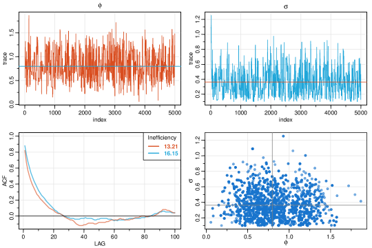
The intuition of our method can be seen in the simulation displayed in Figure 2. That is, rather than sample $\phi$ and $\sigma$ individually, it would be better to sample them at the same time. That is, in the generic Gibbs sampler, we accomplish Procedure 1-(i) by sampling directly from $\operatorname{p}(\phi,\sigma\mid x_{0:n},y_{1:n})$ rather than sampling each parameter separately. As will be seen, this change brings a big improvement to the mixing and convergence problems for SV models.

To accomplish this goal, we put a bivariate normal prior with a negative correlation coefficient on the pair $\Theta=(\phi,\sigma)$,

$$\left(\begin{array}[]{c}\phi\\ \sigma\end{array}\right)\sim\operatorname{N}_{2}\Biggl{(}\biggl{[}\begin{array}[]{c}\mu_{\phi}\\ \mu_{q}\end{array}\biggr{]},\begin{bmatrix}\sigma_{\phi}^{2}&\rho\sigma_{\phi}\sigma_{q}\\ \rho\sigma_{\phi}\sigma_{q}&\sigma_{q}^{2}\end{bmatrix}\Biggr{)},$$ (8)

where typically, $\rho<0$. Allowing possible negative values for $\sigma$ is an old trick used in optimization to avoid constraints on the parameter space. The trick is reasonable because $\sigma^{2}$ will always be non-negative and has a scaled chi-squared prior distribution. In addition, as is seen in Figure 2, a bivariate normal prior is sensible. Note that we have changed the notation slightly by excluding $\mu$ from $\Theta=(\phi,\sigma)$ because it may be sampled separately if necessary.

To accomplish Procedure 1-(i), note that,

$$\operatorname{p}(\Theta,\mu\mid x_{0:n},y_{1:n})\propto\pi(\Theta,\mu)\,\operatorname{p}(x_{0}\mid\Theta,\mu)\,\prod_{t=1}^{n}\operatorname{p}(x_{t}\mid x_{t-1},\Theta,\mu)\,\operatorname{p}(y_{t}\mid x_{t},\Theta,\mu)\,,$$ (9)

where $\pi(\Theta,\mu)$ is the prior on the parameters. For the generic state space model, the parameters are often taken to be conditionally independent with distributions from standard parametric families (at least as long as the prior distribution is conjugate relative to the model specification). In this case, however, we must work with non-conjugate models, and one option is to replace Procedure 1-(i) with a Metropolis-Hastings step, which is feasible because the complete data density $\operatorname{p}(\Theta,\mu,x_{0:n},y_{1:n})$ can be evaluated pointwise.

Under these considerations, for the SV model in (2)–(3), we have

$$\operatorname{p}(\Theta\mid\mu,x_{0:n},y_{1:n}) \propto\pi(\Theta)\operatorname{p}(x_{0}\mid\Theta,\mu)\prod_{t=1}^{n}\operatorname{p}(x_{t}\mid x_{t-1},\Theta,\mu)$$

$$\propto\exp\Biggl{\{}-\frac{1}{2(1-\rho^{2})}\biggl{[}\frac{(\phi-\mu_{\phi})^{2}}{\sigma_{\phi}^{2}}+\frac{(\sigma-\mu_{\sigma})^{2}}{\sigma_{q}^{2}}-\frac{2\rho(\phi-\mu_{\phi})(\sigma-\mu_{\sigma})}{\sigma_{\phi}\sigma_{q}}\biggr{]}\Biggr{\}}$$

$$\cdot\frac{\sqrt{1-\phi^{2}}}{\sigma}\exp\biggl{\{}-\frac{(x_{0}-\mu)^{2}}{2\sigma^{2}/(1-\phi^{2})}\biggr{\}}\prod_{t=1}^{n}\frac{1}{\sigma}\exp\biggl{\{}-\frac{[(x_{t}-\mu)-\phi(x_{t-1}-\mu)]^{2}}{2\sigma^{2}}\biggr{\}}$$

$$\propto\exp\Biggl{\{}-\frac{(\phi-\mu_{\phi})^{2}\sigma_{q}^{2}+(\sigma-\mu_{\sigma})^{2}\sigma_{\phi}^{2}-2\rho\sigma_{\phi}\sigma_{q}(\phi-\mu_{\phi})(\sigma-\mu_{\sigma})}{2(1-\rho^{2})\sigma_{\phi}^{2}\sigma_{q}^{2}}\Biggr{\}}$$

$$\cdot\frac{\sqrt{1-\phi^{2}}}{\sigma^{n}}\exp\biggl{\{}-\frac{(1-\phi^{2})(x_{0}-\mu)^{2}+\sum_{t=1}^{n}[(x_{t}-\mu)-\phi(x_{t-1}-\mu)]^{2}}{2\sigma^{2}}\biggr{\}}.$$ (10)

As previously suggested, we use a random walk Metropolis step to sample $\Theta=(\phi,\sigma)$ simultaneously from the target posterior distribution $\operatorname{p}(\Theta\mid\mu,x_{0:n},y_{1:n})$ given in (10). This approach involves choosing a tuning parameter to control the acceptance probability. However, sometimes a good proposal distribution is difficult to choose because both the size and the spatial orientation of the proposal distribution should be considered. We have found that, for large samples, the use of an adaptive method can help with the problem. We suggest using a technique that was presented in Andrieu and Thoms, (2008, Alg. 4) and is displayed in Procedure 5 for our case.

Procedure 5 (Adaptive Normal Random Walk Metropolis).

Input: Initial value, $\Theta_{0}$, and an initial bivariate normal proposal distribution $\operatorname{N}_{2}(\mu_{0},\lambda_{0}\Sigma_{0})$.
On iteration $j+1$, for $j=0,1,2,\dots$,

1. Draw $\vartheta\sim\operatorname{N}_{2}(\Theta_{j},\lambda_{j}\Sigma_{j})$ and set $\Theta_{j+1}=\vartheta$ with probability $\alpha_{j+1}=\frac{g(\vartheta)}{g(\Theta_{j})}\wedge 1$, where $g(\Theta)$ is given on the rhs of (10). Otherwise, set $\Theta_{j+1}=\Theta_{j}$

2. [Optional]  Update

   $$\log(\lambda_{j+1}) =\log(\lambda_{j})+\gamma_{j+1}[\alpha_{j+1}-\alpha_{\star}],$$ (11)

   $$\mu_{j+1} =\mu_{j}+\gamma_{j+1}(\Theta_{j+1}-\mu_{j}),$$ (12)

   $$\Sigma_{j+1} =\Sigma_{j}+\gamma_{j+1}[(\Theta_{j+1}-\mu_{j})(\Theta_{j+1}-\mu_{j})^{\prime}-\Sigma_{j}],$$ (13)

   where $\gamma_{j}$ is a scalar nonincreasing sequence of positive step lengths such that $\sum_{j=1}^{\infty}\gamma_{j}=\infty$ and $\sum_{j=1}^{\infty}\gamma_{j}^{1+\delta}<\infty$ for some $\delta>0$; $\alpha_{\star}$ is the expected acceptance rate for the algorithm.

Optionally, one may fix $\lambda_{j}$ and $\Sigma_{j}$ and skip step Procedure 5-(ii) if it is not necessary. The optional part makes the algorithm non-Markovian, however, it can adapt continuously to the target distribution. Both the size and the spatial orientation of the proposal distribution will be adjusted by the adaptation procedure. Also, Procedure 5 is straightforward to implement and to use in practice. There are no extra computational costs because only a simple recursion formula for the covariances involved. The algorithm starts by using the accumulating information from the beginning of the sampling and it ensures that the search becomes more efficient at an early stage of the sampling. Haario et al., (2001) establish that the adaptive MCMC algorithms do indeed have the correct ergodicity properties.

If the leverage parameter, $\mu$, is included in the model, using a diffuse prior (e.g., see Kim et al.,, 1998), we have

$$\mu\mid\Theta,x_{0:n},y_{1:n}\sim N(\nu_{\mu},\sigma_{\mu}^{2})$$ (14)

where

$$\nu_{\mu}=\sigma_{\mu}^{2}\bigg{\{}\frac{1-\phi^{2}}{\sigma^{2}}x_{0}+\frac{1-\phi}{\sigma^{2}}\sum_{t=1}^{n}(x_{t}-\phi x_{t-1})\bigg{\}}$$

and

$$\sigma_{\mu}^{2}=\frac{\sigma^{2}}{n(1-\phi)^{2}+(1-\phi^{2})}.$$

Recall that we are fixing $\beta=\exp(\mu/2)$. Finally, our algorithm for the analysis of a univariate SV model is given in Algorithm 1.

Input: Set the initial value of $\Theta^{[0]}=(\phi,\sigma)^{[0]},\mu^{[0]},$ and $x_{0:n}^{[0]}$ arbitrarily.

At iteration $j=1,2,\dots$,

1. Draw $x_{0:n}^{[j]}$ by CPF-AS, Procedure 4, conditioned on $x_{0:n}^{[j-1]}$ and $\Theta^{[j-1]},\mu^{[j-1]}$.

2. With $x_{0:n}^{[j]}$, generate $\Theta^{[j]}=(\phi,\sigma)^{[j]}$ via Procedure 5 and draw $\mu^{[j]}$ from the posterior given in (14) under the current draws $x_{0:n}^{[j]}$ and $\Theta^{[j]}$.

Algorithm 1 Joint Particle Gibbs for Univariate Stochastic Volatility Models

4 Examples

4.1 Joint versus Individual Sampling for a Two Parameter Model

In this section, we fit a two-parameter model ($\mu=0$) to the daily returns of the S&P 500 from January 2005 to October of 2011 shown at the top of Figure 3. The data include the financial crisis of 2008. We compare two particle Gibbs methods using CPF-AS (Procedure 4) to sample the state process in both. The standard (existing) method samples the parameters individually by drawing from the univariate posteriors $\operatorname{p}(\phi\mid\sigma,x_{0:n},y_{1:n})$ and $\operatorname{p}(\sigma\mid\phi,x_{0:n},y_{1:n})$ while our method samples the parameters jointly as described in Algorithm 1 holding $\mu$ at zero.

In each case, we used $N=20$ particles for the CPF-AS (Procedure 4) and 5000 iterations after a burnin of 100. The posterior mean and a pointwise 95% credible interval of the draws of the state (log-volatility) process is shown in Figure 3. The middle plot shows the results for the existing method and the bottom plot shows the results for our proposed method. The results are similar, but the trace of the estimated process is smoother and less variable than existing method shown in the middle.

Figure 3: top: Daily returns of the S&P 500 from January 2005 to October of 2011. middle: State process estimated posterior mean and pointwise 95% credible intervals based on the existing method of one-at-a-time parameter sampling. bottom: State process estimated posterior mean and pointwise 95% credible intervals based on the proposed method of joint parameter sampling, Algorithm 1. The number of particles used in the particle filter (Procedure 4) for both methods was $N=20$.

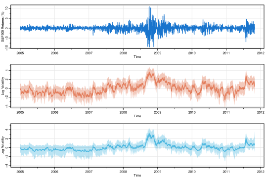
Figure 4 displays the results of the parameter estimation using the standard method of sampling $\phi$ and $\sigma$ separately. The top of the figure shows the traces of the sampled values after burnin. The corresponding posterior means are $.88$ for $\phi$ and $.62$ for $\sigma$. The bottom of the figure shows the sample ACFs of the traces and a scatterplot of the sampled values. In addition, the ACF plot displays the inefficiency measure as defined in Geyer, (1992). The measure was obtained using Geyer’s R package, mcmc (Geyer and Johnson,, 2017). In particular, to evaluate the mixing of sampler, we estimate inefficiency defined as

$$\text{IF}:=1+2\sum_{i=1}^{\infty}\rho(i),$$ (15)

where $\rho(i)$ is the autocorrelation function of the trace at lag $i$. The estimated inefficiencies are displayed with the sample ACFs of traces. We note again the slow convergence problem seen in the simulation example, Figure 2, and reported in Chib and Greenberg, (1996) and Kim et al., (1998). Finally, the bottom right scatterplot shows the strong correlation between the individually sampled parameters.

Figure 4: (Individual Sampling) S&P 500, results of the parameter estimation in a two-parameter model using the standard method of sampling $\phi$ and $\sigma$ separately. The top shows the traces of the 5000 sampled values after a burnin of 100. The number of particles used in the particle filter (Procedure 4) was $N=20$. The corresponding posterior means are $.88$ for $\phi$ and $.62$ for $\sigma$. The bottom left shows the sample ACFs of the traces and the estimated inefficiency measure as defined in (15). The bottom left shows a scatterplot of the sampled parameters, and exhibits strong negative correlation.

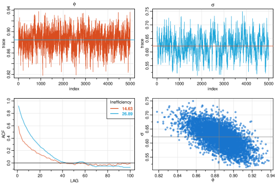
Figure 5 displays the results of the parameter estimation using our proposed method, Algorithm 1, sampling $\phi$ and $\sigma$ simultaneously. The top of the figure shows the traces of the sampled values after burnin. The corresponding posterior means are $.80$ for $\phi$ and $.36$ for $\sigma$. The bottom of the figure shows the sample ACFs of the traces and a scatterplot of the sampled values, which shows an improvement of the established method. While the inefficiencies of estimating $\phi$ are similar, the inefficiencies of estimating $\sigma$ are much improved. In addition, the scatterplot of the joint draws of the parameters shows the absence of correlation among the samples.

Figure 5: (Joint Sampling) S&P 500, results of the parameter estimation in a two-parameter model using the proposed method of sampling $\phi$ and $\sigma$ jointly, Algorithm 1. The top shows the traces of the 5000 sampled values after a burnin of 100. The number of particles used in the particle filter (Procedure 4) was $N=20$. The corresponding posterior means are $.80$ for $\phi$ and $.36$ for $\sigma$. The bottom shows the sample ACFs of the traces and a scatterplot of the sampled values, which indicate the sample parameters are uncorrelated. In addition, estimated inefficiency measures are improved over the counterparts in Figure 4.

4.2 Three Parameter Model

Next, we fit a three parameter SV model to the S&P 500 series using Algorithm 1, however, the adaptive part of the Metropolis step, Procedure 5-(ii), was skipped. To keep the complexity low, we used only $N=10$ particles for sampling the states (Procedure 4), and then generated 2000 samples after a burnin of 100. The acceptance rate was nearly optimal at $26.1\%$. The entire estimation process took less than 4 minutes on a workstation running Windows 10 Pro with 32GB of DDR3 RAM, an Intel i7-4770 CPU @ 3.40 GHz, and using Microsoft R, version 3.5.2.

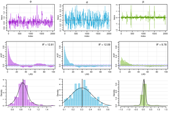
The results of the parameter estimation are shown in Figure 6; the results for the state estimation are similar to the lower plot of Figure 3 and are not shown to save space. The figure shows the trace of the draws (top row), the sample ACF of the draws (middle row) along with the estimated inefficiency, (15), and a histogram of the results (bottom row). The posterior means are displayed in the figure and were $.85$ for $\phi$, $.30$ for $\sigma$ and $.05$ for $\mu$. We note that the results are satisfactory even using this quick analysis. In addition, it is apparent that the previous analysis based on the two-parameter model ($\mu=0$) was reasonable.

Figure 6: S&P 500, results of the parameter estimation in a three-parameter model using the proposed method of sampling $\phi$ and $\sigma$ jointly, Algorithm 1. top: Traces of the 2000 sampled values of the parameters after burnin. middle: Sample ACF of the draws along with the estimated inefficiency, (15). bottom: Histogram of the results. The posterior means are displayed in the figure and were $.85$ for $\phi$, $.30$ for $\sigma$ and $.05$ for $\mu$.

5 Multivariate Stochastic Volatility Model

It is often reasonable to assume that similar assets are being driven by the same volatility process. In this case, the multivariate stochastic volatility (MSV) model presented in Asai et al., (2006) can be used. The model assumes a univariate volatility process is driving a number of similar assets and is given by,

$$x_{t} =\phi x_{t-1}+\sigma w_{t}$$ (16)

$${y}_{it} =\beta_{i}\exp\Bigl{\{}\frac{x_{t}}{2}\Bigr{\}}\,\epsilon_{it}\,,\quad i=1,\dots,p,$$ (17)

where the $y_{it}$ are the returns of the $i$th asset, $w_{t}\stackrel{{\scriptstyle\mathrm{iid}}}{{\sim\,}}\operatorname{N}(0,1)$, and $\boldsymbol{\epsilon}_{t}=(\epsilon_{1t},\dots,\epsilon_{pt})^{\prime}\stackrel{{\scriptstyle\mathrm{iid}}}{{\sim\,}}\operatorname{N}_{p}(0,\mathrm{I})$. In this model, the leverage ($\mu$) is removed to avoid overparameterization and each $\beta_{i}$ is a scale parameter for the $i$th asset.

We can easily apply our proposed method to the MSV model. That is, as in the univariate case, we put a bivariate normal prior on the state parameters, $\phi$ and $\sigma$. Then, because $\beta_{i}$, for $i=1,\dots,p$, is a scale parameter, a reasonable choice is to use independent inverse gamma priors for $\beta_{i}^{2}$ as in (6). That is, if $\beta_{i}^{2}\sim{\rm IG}(a_{i}/2,b_{i}/2)$, then the posterior is

$$\beta_{i}^{2}\mid\Theta,x_{0:n},y_{1:n}\sim{\rm IG}\Bigl{(}\tfrac{1}{2}(a_{i}+n+1),\ \tfrac{1}{2}\Bigl{\{}b_{i}+\sum_{t=1}^{n}\frac{y_{it}^{2}}{\exp(x_{t})}\Bigr{\}}\Bigr{)}\,.$$ (18)

Hence, in the MSV model, we can simply add a third step to Algorithm 1, which is to sample $\beta_{i}^{2}$ from (18) for $i=1,\dots,p$. We summarize these steps in Algorithm 2.

Input: Set the initial value of $\Theta^{[0]}=(\phi,\sigma)^{[0]},$ $\beta_{1:p}^{[0]}$, and $x_{0:n}^{[0]}$ arbitrarily.

At iteration $j=1,2,\dots$,

1. Draw $x_{0:n}^{[j]}$ by CPF-AS, Procedure 4, conditioned on $x_{0:n}^{[j-1]}$ and $\Theta^{[j-1]}$.

2. With $x_{0:n}^{[j]}$, generate $\Theta^{[j]}=(\phi,\sigma)^{[j]}$ via Procedure 5 and draw $\beta_{1:p}^{2\,[j]}$ from the posteriors given in (18) under the current draws $x_{0:n}^{[j]}$ and $\Theta^{[j]}$.

Algorithm 2 Joint Particle Gibbs for Multivariate Stochastic Volatility Models

Figure 7: The daily NYSE returns (as percentages) for three banks, Bank of American (BOA), Citigroup (Citi), and J.P. Morgan (JPM) from January 2005 to November 2017. bottom: The resulting posterior of the log-volatility based on Algorithm 2. Shown are the posterior mean and a swatch displaying the limits of $99\%$ of the sampled states. We also display a lowess smooth as a thin line to emphasize the volatility trend.

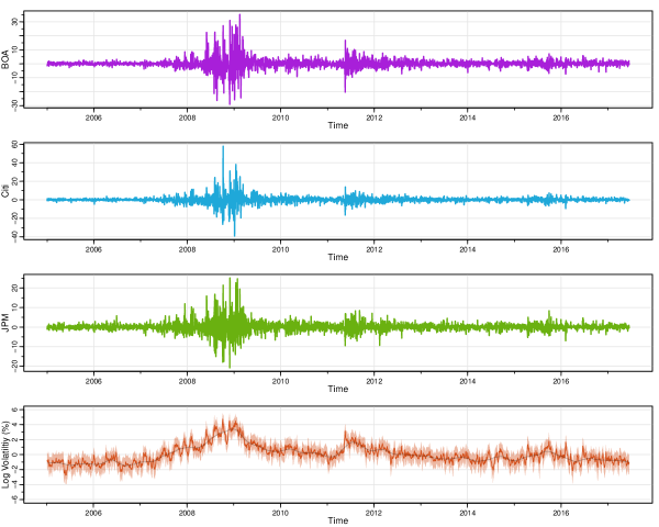
For an example, we consider the daily NYSE returns for three banks, Bank of American (BOA), Citigroup (Citi), and J.P. Morgan (JPM) from January 2005 to November 2017. The data are displayed in Figure 7; also shown is the estimated log-volatility, which we describe shortly.

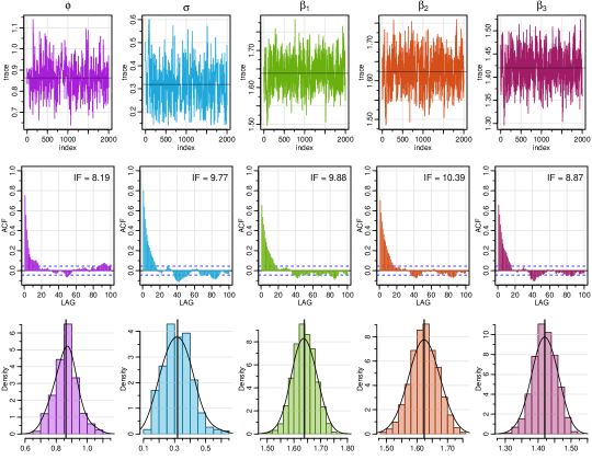
We used Algorithm 2 with $N=20$ particles to generate 2000 draws after a burnin of 500 iterations. The procedure was non-adaptive and the acceptance rate was $29.8\%$. The entire procedure took about 12 minutes on the same machine mentioned in the other examples. The parameter estimation summary is displayed in Figure 8 and the display is similar to the previous example. The displays suggest that the algorithm is mixing well. The top shows the traces of the draws for each parameter and indicates the posterior means, $.86$ for $\phi$, $.32$ for $\sigma$, and $1.64$, $1.62$, and $1.42$ for the $\beta$s of BOA, Citi, and JPM, respectively. The middle plot shows the sample ACFs of the traces along with the inefficiencies. The bottom row of Figure 8 displays the posterior distributions of each parameter along with the location of the posterior mean.

The resulting posterior of the log-volatility is shown at the bottom of Figure 7. Shown are the posterior mean and a swatch displaying pointwise $99\%$ credible intervals. We also display a lowess fit as a thin line to emphasize the volatility trend. Notice that the impending financial crisis of 2008 is visible at least one year prior as the volatility starts a trend upwards just prior to 2007. It seems that there is an advantage to using multiple similar sources to estimate volatility.

Figure 8: For the bank returns data shown in Figure 7, the results of fitting an MSV model based on Algorithm 2. top: The traces of the draws for each parameter and indicates the posterior means, $.86$ for $\phi$, $.32$ for $\sigma$, and $1.64$, $1.62$, and $1.42$ for the $\beta$s of BOA, Citi, and JPM, respectively. middle: The sample ACFs of the traces along with the inefficiencies. bottom: The estimated posterior distributions of each parameter along with the location of the posterior mean.

6 Conclusions

The conditional particle filter with ancestral sampling (Procedure 4) was a breakthrough for analyzing nonlinear state space models by establishing a computationally efficient method of sampling from the posterior of the hidden state trajectories, Procedure 1-(ii). The method works well for many cases if drawing from the posterior of the parameters, Procedure 1-(i), is not problematic. Unfortunately, this situation does not include the case of stochastic volatility models because in the state equation, the autoregressive parameter, $\phi$ and the noise variance, $\sigma^{2}$ in (2) have a tendency to work in opposite directions.

Prior attempts to handle SV models had efficiency problems because $\phi$ was treated as a regression parameter while $\sigma$ was treated as a scale parameter. Consequently, these parameters were sampled individually as they typically are in these situations. For many state space models, this treatment of the problem is fine. For SV models however, this approach is an efficiency nightmare.

We have presented a method to overcome this problem by sampling the state parameters jointly. We used a bivariate normal distribution based on the fact that it is easy to work with in that it captures the subtleties of the relationship, but also, as seen in Figure 4, $\phi$ and $\sigma$ live on ellipses. While it is possible that a sampled pair yields values of $|\phi|>1$ or $\sigma<0$, it does not appear to be a problem. For example, the state process is assumed to be stationary, so realistically, one only needs $|\phi|\neq 1$, which will not happen (with probability 1 in all but pathological cases). Also, sampled values of $\sigma^{2}$ will always be non-negative. We do note that, even though $\sigma$ was small in our examples, we never saw a negative value of $\sigma$.

Finally, we mention that we did not supply every particular numerical detail (e.g., hyperparameters and tuning parameters) of our examples. Instead, for the sake of reproducibility, we supply the R code for every example on GitHub; see Gong and Stoffer, (2019) for the url. Additional information may also be found in Gong, (2019).

References

- Andrieu et al., (2010) Andrieu, C., Doucet, A., and Holenstein, R. (2010). Particle Markov chain Monte Carlo methods. Journal of the Royal Statistical Society: Series B (Statistical Methodology), 72(3):269–342.
- Andrieu and Thoms, (2008) Andrieu, C. and Thoms, J. (2008). A tutorial on adaptive MCMC. Statistics and Computing, 18(4):343–373.
- Asai et al., (2006) Asai, M., McAleer, M., and Yu, J. (2006). Multivariate stochastic volatility: a review. Econometric Reviews, 25(2-3):145–175.
- Carlin et al., (1992) Carlin, B. P., Polson, N. G., and Stoffer, D. S. (1992). A Monte Carlo approach to nonnormal and nonlinear state-space modeling. Journal of the American Statistical Association, 87(418):493–500.
- Carter and Kohn, (1994) Carter, C. K. and Kohn, R. (1994). On Gibbs sampling for state space models. Biometrika, 81(3):541–553.
- Chib and Greenberg, (1996) Chib, S. and Greenberg, E. (1996). Markov chain Monte Carlo simulation methods in econometrics. Econometric Theory, 12(3):409–431.
- Del Moral, (1996) Del Moral, P. (1996). Non-linear filtering: Interacting particle resolution. Markov Processes and Related Fields, 2(4):555–581.
- Douc et al., (2014) Douc, R., Moulines, E., and Stoffer, D. S. (2014). Nonlinear Time Series: Theory, Methods and Applications with R Examples. CRC Press, Boca Raton.
- Doucet et al., (2000) Doucet, A., Godsill, S., and Andrieu, C. (2000). On sequential Monte Carlo sampling methods for Bayesian filtering. Statistics and Computing, 10(3):197–208.
- Frühwirth-Schnatter, (1994) Frühwirth-Schnatter, S. (1994). Data augmentation and dynamic linear models. Journal of Time Series Analysis, 15(2):183–202.
- Geyer, (1992) Geyer, C. J. (1992). Practical Markov chain Monte Carlo. Statist. Sci., 7(4):473–483.
- Geyer and Johnson, (2017) Geyer, C. J. and Johnson, L. T. (2017). mcmc: Markov Chain Monte Carlo. R package version 0.9-5.
- Godsill et al., (2004) Godsill, S. J., Doucet, A., and West, M. (2004). Monte Carlo smoothing for nonlinear time series. Journal of the American Statistical Association, 99(465):156–168.
- Gong, (2019) Gong, C. (2019). Particle Gibbs Methods in Stochastic Volatility Models. PhD thesis, University of Pittsburgh.
- Gong and Stoffer, (2019) Gong, C. and Stoffer, D. S. (2019). Stochastic Volatility Models. https://github.com/nickpoison/Stochastic-Volatility-Models/. [GitHub Repository].
- Gordon et al., (1993) Gordon, N., Salmond, D., and Smith, A. F. (1993). Novel approach to nonlinear/non-Gaussian Bayesian state estimation. IEE Proc. F, Radar Signal Process., 140:107–113.
- Haario et al., (2001) Haario, H., Saksman, E., and Tamminen, J. (2001). An adaptive Metropolis algorithm. Bernoulli, 7(2):223–242.
- Jacquier et al., (1994) Jacquier, E., Polson, N. G., and Rossi, P. E. (1994). Bayesian analysis of stochastic volatility models. Journal of Business & Economic Statistics, 20(1):69–87.
- Kastner and Hosszejni, (2019) Kastner, G. and Hosszejni, D. (2019). stochvol: Efficient Bayesian Inference for Stochastic Volatility (SV) Models. R package version 2.0.4.
- Kim et al., (1998) Kim, S., Shephard, N., and Chib, S. (1998). Stochastic volatility: Likelihood inference and comparison with ARCH models. The Review of Economic Studies, 65(3):361–393.
- Lindsten et al., (2014) Lindsten, F., Douc, R., and Moulines, E. (2014). Particle Gibbs with ancestor sampling. Journal of Machine Learning Research, 15:2145–2184.
- Lindsten et al., (2013) Lindsten, F., Schön, T. B., et al. (2013). Backward simulation methods for Monte Carlo statistical inference. Foundations and Trends in Machine Learning, 6(1):1–143.
- Liu and Chen, (1998) Liu, J. S. and Chen, R. (1998). Sequential Monte Carlo methods for dynamic systems. Journal of the American Statistical Association, 93(443):1032–1044.
- Pitt and Shephard, (1999) Pitt, M. K. and Shephard, N. (1999). Filtering via simulation: Auxiliary particle filters. Journal of the American Statistical Association, 94(446):590–599.
- Shephard, (1996) Shephard, N. (1996). Statistical aspects of ARCH and stochastic volatility. Monographs on Statistics and Applied Probability, 65:1–68.
- Shumway and Stoffer, (2017) Shumway, R. H. and Stoffer, D. S. (2017). Time Series Analysis and Its Applications: With R Examples. Springer, New York, 4th edition.
- Taylor, (1994) Taylor, S. J. (1994). Modeling stochastic volatility: A review and comparative study. Mathematical Finance, 4(2):183–204.
- Taylor, (2008) Taylor, S. J. (2008). Modelling Financial Time Series. World Scientific, 2nd edition.
- Whiteley et al., (2010) Whiteley, N., Andrieu, C., and Doucet, A. (2010). Efficient Bayesian inference for switching state-space models using discrete particle Markov chain Monte Carlo methods. arXiv preprint arXiv:1011.2437.