ALMA Observations of the Terahertz Spectrum of Sagittarius A*

Abstract

We present ALMA observations at 233, 678, and 870 GHz of the Galactic Center black hole, Sagittarius A*. These observations reveal a flat spectrum over this frequency range with spectral index $\alpha\approx-0.3$, where the flux density $S\propto\nu^{\alpha}$. We model the submm and far infrared spectrum with a one zone synchrotron model of thermal electrons. We infer electron densities $n=(2-5)\times 10^{6}$ cm^-3, electron temperatures $T_{e}=(1-3)\times 10^{11}$ K, and magnetic field strength $B=10-50$ G. The parameter range can be further constrained using the observed quiescent X-ray luminosity. The flat submm spectrum results in a high electron temperature and implies that the emitting electrons are efficiently heated. We also find that the emission is most likely optically thin at 233 GHz. These results indicate that millimeter and submillimeter wavelength very long baseline interferometry of Sgr A* including those of the Event Horizon Telescope should see a transparent emission region down to event horizon scales.

1 Introduction

The Galactic center compact radio source, Sagittarius A* (Sgr A*, Balick & Brown, 1974) is the prototype for low-luminosity accretion onto a massive black hole (Yuan & Narayan, 2014). Its inverted radio spectrum rises to a submillimeter (submm) or far-infrared peak (Falcke et al., 1998; Bower et al., 2015a). The radio source varies with an rms rising from $\simeq 10\%$ in the radio (Herrnstein et al., 2004; Macquart & Bower, 2006; Bower et al., 2015a) to $\simeq 30\%$ at 230 GHz (Zhao et al., 2003; Marrone et al., 2008; Eckart et al., 2008; Dexter et al., 2014) to an order of magnitude in the near-infrared and factors of a hundred or thousand in X-rays (Dodds-Eden et al., 2011; Neilsen et al., 2015; Witzel et al., 2018). Millimeter and submillimeter wavelength linear and circular polarization measurements have provided important diagnostics of the emitting plasma and the accretion flow on scales out to the Bondi radius (Aitken et al., 2000; Bower et al., 1999, 2003; Macquart et al., 2006; Marrone et al., 2007a; Muñoz et al., 2012; Bower et al., 2018). The emission size decreases with wavelength (Krichbaum et al., 1998; Shen et al., 2005; Bower et al., 2006, 2014; Johnson et al., 2018), with a size $\simeq 40-50\mu$as at 230 GHz corresponding to roughly 8 gravitational radii ($r_{g}=GM/c^{2}$) (Krichbaum et al., 1998; Doeleman et al., 2008; Lu et al., 2018), making Sgr A* a prime target for studying accretion and strong gravity on event horizon scales (Falcke et al., 2000; Johannsen & Psaltis, 2010). The first such test was recently performed with the discovery of near-infrared flares orbiting the black hole at $\simeq 6-10r_{g}$ (Gravity Collaboration et al., 2018a). Event Horizon Telescope imaging of the black hole in M87 demonstrates the capability for similar imaging of Sgr A* (Event Horizon Telescope Collaboration et al., 2019a, b, c, d, e, f).

Intensive studies of Sgr A* from radio to X-ray wavelengths provide tests of accretion (Melia et al., 1998; Narayan et al., 1995; Quataert & Narayan, 1999; Özel et al., 2000; Yuan et al., 2003) and outflow (Falcke & Markoff, 2000) models. The development of general relativistic MHD simulations of black hole accretion flows (GRMHD, De Villiers et al., 2003; Gammie et al., 2003) has led to a large effort in comparing those models to data, including the variable submm spectral energy distribution (SED) (e.g., Noble et al., 2007; Dexter et al., 2009, 2010; Mościbrodzka et al., 2009; Mościbrodzka & Falcke, 2013; Shcherbakov et al., 2012; Drappeau et al., 2013a; Chan et al., 2015).

One of the most important constraints for the models is the location and spectral shape near the peak of the SED. Past observations have characterized the time variable SED, but with only a few simultaneous measurements in multiple submm bands (Marrone, 2006). These measurements along with recent data from ALMA (Bower et al., 2015a; Liu et al., 2016a) and detections of variable flux from Sgr A* in the far-infrared (Stone et al., 2016; von Fellenberg et al., 2018) suggest that the peak lies somewhere in the THz range. The submm bump is also found to be less peaked than previously thought, which implies a higher electron temperature and an optically thin emission region near the peak of the SED.

Here we report flux density measurements from ALMA observations of Sgr A* simultaneous at 233 and 678 GHz, as well as a precise measurement at 868 GHz, the first at that frequency using an interferometer (Section 2). Interferometric observations at THz frequencies have the advantage of high angular resolution over single dish observations, which is important for separating the compact source from the extended and bright Galactic Center emission. In cases where phase self-calibration is possible, interferometers also provide better calibration through rejection of temporally and spatially variable atmospheric emission. We show that the simultaneous 233 and 678 GHz measurements are consistent with and more precise than earlier ones using the SMA. The 868 GHz flux density is somewhat lower than previously found at 850 GHz with the CSO, possibly as the result of unsubtracted extended flux density. From our data, we show that the spectral peak occurs at a frequency $\gtrsim 900$ GHz. Combined with upper limits from Herschel SPIRE and PACs, we use a one zone model of synchrotron radiation from a thermal population of electrons to infer the source properties (Section 3). We show that the spectral peak occurs at $\simeq 1-2$ THz, and that the emission region is likely optically thin for frequencies $\gtrsim 230$ GHz.

2 Observations, Data Reduction, and Results

Observations of Sgr A* were obtained on two days in March 2017 as part of ALMA Cycle 4. On 18 March 2017, observations were obtained in Band 10 (868 GHz). Weather was excellent for the Band 10 measurements with 0.29 mm precipitable water vapor (PWV). On 22 March 2017, observations were obtained in Bands 6 and 9 (233 and 678 GHz, respectively) within 45 minutes of each other. For all three bands, integrations on Sgr A* were 2 minutes in each band; calibrator integrations were of comparable duration.

Observations in each band were obtained in standard correlator configurations with four spectral windows (SPWs) each with 2 GHz bandwidth and 128 channels. Data were obtained in two orthogonal linear polarizations but correlations were computed only for parallel hands.

Data reduction was performed using CASA, following standard procedures for flux, gain, and bandpass calibration, including phase self-calibration on short time scales for Sgr A* and each calibrator. Flux calibration is based on estimates of the flux density of the ALMA gain calibrator J1924-2914, which was observed primarily in Bands 3 and 7 (90 GHz and 345 GHz, respectively) and then extrapolated to our observing bands. In Figure 1, we compare the measured flux density on J1924-2914 against archival measurements. Comparisons to archival ALMA Band 6 measurements for all calibrators show excellent consistency with differences to nearest measurements $\stackrel{{\scriptstyle\scriptstyle<}}{{\scriptstyle\sim}}10\%$. There are no Band 9 and 10 measurements within one year of our measurements for any of the calibrators. There are a pair of Band 9 measurements for J1924-2914 from two years prior that agree within 10% of the extrapolated flux (and resultant measurement). The measured Band 10 flux density of J1751+0939 $S=1.31\pm 0.01$ Jy agrees with the ALMA calibrator database Bands 3 and 7 extrapolated flux density of $S=1.34$ Jy. We estimate that systematic flux density errors in Bands 9 and 10 are $\stackrel{{\scriptstyle\scriptstyle<}}{{\scriptstyle\sim}}20\%$.

Table 1: Flux Measurements and Spectral Indices

Source	$S_{233}$	$S_{678}$	$S_{868}$	$\alpha$
	(mJy)	(mJy)	(mJy)
J1700-2610	…	…	$0.426\pm 0.019$	…
J1733-1304	$1.592\pm 0.045$	…	…	…
J1733-3722	…	$0.353\pm 0.009$	…	…
J1744-3116	$0.270\pm 0.008$	$0.096\pm 0.006$	$0.058\pm 0.009$	$-1.11\pm 0.07$
J1751+0939	…	…	$1.311\pm 0.008$	…
J1924-2914	$3.312\pm 0.086$	$1.819\pm 0.004$	$1.342\pm 0.051$	$-0.65\pm 0.03$
Sgr A*	$2.886\pm 0.043$	$2.183\pm 0.026$	$1.864\pm 0.067$	$-0.31\pm 0.02$

Note. — $\alpha$ is determined over all three frequency bands. Note that the 233 and 678 GHz observations were obtained on the same day but 868 GHz observations were obtained on a different day.

Images of Sgr A* in Bands 9 and 10 were point sources, while Sgr A West is apparent in the Band 6 data. Given that these are all just a few minute snapshots they do not present very interesting opportunities for imaging. The rms noise levels in the images in Bands 6, 9, and 10 were 4, 5, and 14 mJy, respectively. The array was in a compact configuration with maximum baseline of 2.4 km. This produced a naturally-weighted synthesized beam of $\sim 1.5$ arcsec in Band 6, $\sim 0.5$ arcsec in Band 9, and $\sim 0.4$ arcsec in Band 10.

Flux densities were fit for each source in each spectral window using a point source model in the visibility domain. Figure 2 shows all flux densities measured. In Table 1, we report mean flux densities in each band. Errors are computed from the scatter in measurements, which provides more accurate assessment of errors than propagation of statistical uncertainties.

We also compute the spectral index $\alpha$ (using $S\propto\nu^{\alpha}$) for sources with measurements in all three bands. The spectrum of Sgr A* is close to flat with a spectral index $\alpha=-0.3$ across all 3 bands. In comparison, the assumed spectrum of J1924-2914 and the measured spectrum of J1744-3116 are both steeper with $\alpha=-0.7$ and $\alpha=-1.1$, respectively. Considering only the simultaneous 233 and 678 GHz Sgr A* data, $\alpha=-0.26\pm 0.02$.

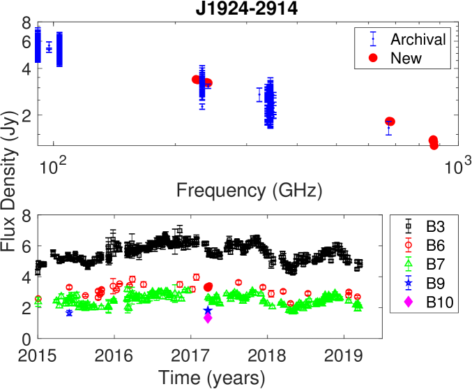
Figure 1: Flux density measurements for the flux calibrator J1924-2914 from these observations and archival ALMA data from January 2015 to March 2019. The top panel shows the spectrum of all measurements. Filled red circles are the new measurements and blue dots are the archival data. The bottom panel shows the light curves for Bands 3, 6, 7, 9, and 10 corresponding roughly to 90, 230, 345, 678, and 868 GHz, respectively. Filled symbols are the new Band 6, 9, and 10 measurements.

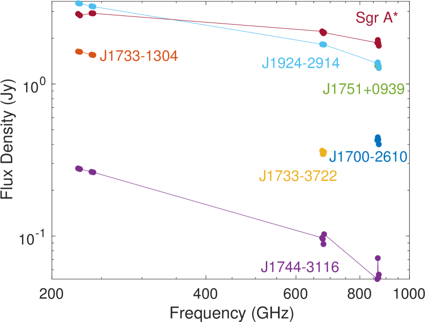
Figure 2: Flux densities for Sgr A* and calibrators from ALMA observations on 18 and 22 March 2017. Flux densities at 870 GHz for J1924-2914 and J1751+0939 are nearly identical and so overlap in the plot.

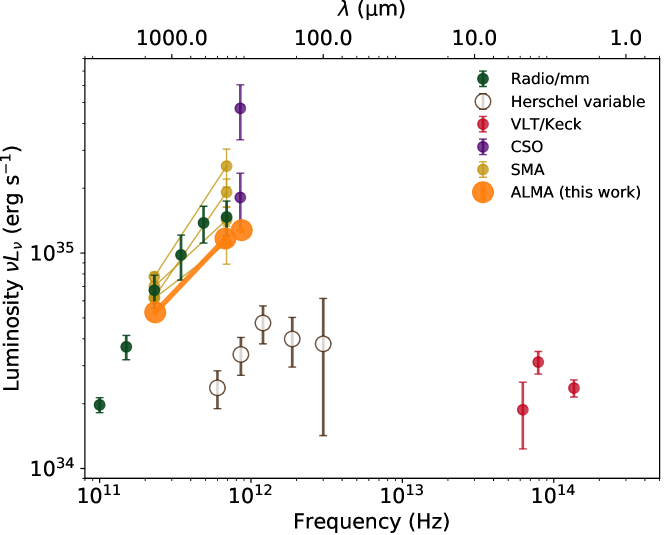
Figure 3: The mm to NIR spectrum of Sgr A*. Orange circles show the new ALMA measurements, with errors much smaller than the symbol size. The green circles show selected radio to submm data (Falcke et al., 1998; Brinkerink et al., 2015; Bower et al., 2015a; Liu et al., 2016a, b). The yellow circles connected with thin lines are simultaneous SMA data (Marrone, 2006). Single dish measurements from CSO at 850 GHz (Serabyn et al., 1997; Yusef-Zadeh et al., 2006) are shown in purple. Detections of variable flux from Sgr A* with Herschel SPIRE (250, 350, 500 micron, Stone et al., 2016) and PACS (160 and tentatively 100 micron, von Fellenberg et al., 2018) are shown as brown open symbols under the assumption that they represent lower limits on the flux density at these frequencies. Near-infrared median flux density measurements (Schödel et al., 2011; Dodds-Eden et al., 2011; Witzel et al., 2018) are shown in red.

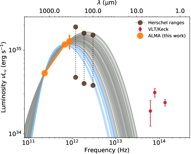
Figure 4: Sample one zone model fits (lines) to our new ALMA measurements and derived flux density ranges from recent Herschel detections of variable flux. The SED peak occurs at 1-2 THz with a bolometric luminosity $\simeq 5\times 10^{35}\,{\rm erg\,s}^{-1}$. The emission region is usually optically thin (gray) rather than optically thick (blue) at 230 GHz. The 68% confidence interval ranges for the plasma parameters are: $n=(2-5)\times 10^{6}\hskip 2.0pt\rm cm^{-3}$, $T_{e}=(1-3)\times 10^{11}$ K, $B=10-50$ G. We note that these parameters are strongly correlated and depend on the chosen emission region size.

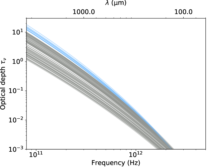
Figure 5: Optical depth $\tau_{\nu}$ as a function of frequency for a sample of our one zone model fits. All models are optically thin at the submm/THz spectral peak, while a small fraction (shown in blue) can be marginally optically thick ($\tau_{\nu}>1$) at 230 GHz.

3 Discussion and Conclusions

We plot our new ALMA submm spectrum of Sgr A* along with measurements from the radio to the NIR (Figure 3). The measured flux density at 230 and 678 GHz are at the low end of the range characterized in previous work (e.g., Marrone, 2006; Dexter et al., 2014; Bower et al., 2015a; Liu et al., 2016b). Previous THz single dish measurements with CSO found higher flux densities (Serabyn et al., 1997; Yusef-Zadeh et al., 2006). The difference with these earlier measurements may be the result of variability or calibration uncertainties associated with THz single dish measurements in this environment with significant extended emission. The characteristic time scale of variability for Sgr A* at 230 GHz and higher frequencies has been measured to be $\tau\approx 8_{-4}^{+3}$ hr (Dexter et al., 2014). Thus, the 45-minute separation between 230 and 678 GHz measurements is nearly simultaneous while the four-day separation with the 868 GHz measurements is significantly longer than the variability coherence time. Long time scale rms variability is approximately 20% (Bower et al., 2015b), which is comparable to the systematic error in the 680-GHz flux density that we estimate. Accordingly, the spectral index of the simultaneous 233 and 678 GHz measurements is the strongest spectral constraint. Still, we note the overall consistency of a power-law spectral index between 233 and 868 GHz in these data.

Our results for Sgr A* are among the best characterized spectrum of any low luminosity AGN (LLAGN) and show one of the flattest spectra for these sources. Doi et al. (2011) characterize the centimeter-to-millimeter wavelength spectra of 21 LLAGN, including 5 with simultaneous data at 100 and 150 GHz, finding flat or inverted spectra for many sources but with no contemporaneous data at frequencies above $>150$ GHz. ALMA observations of M87 extend to 650 GHz and indicate a steep spectrum at frequencies above $\sim 200$ GHz (Prieto et al., 2016). In the case of M94, van Oers et al. (2017) found a flat spectrum up to 100 GHz but place no strong constraints on the spectrum between 100 GHz and the optical as the result of stellar confusion. Contemporaneous observations of the black hole in M81 also indicate a flat spectrum up to 350 GHz but the detailed spectrum is difficult to characterize due to the absence of high angular resolution submillimeter and infrared observations as well as short time scale variability (Markoff et al., 2008; Bower et al., 2015a). Israel et al. (2008) find for the nuclear region of Cen A, a spectral index of $\alpha=-0.2$ to -0.6 between 90 and 230 GHz. Similarly, Espada et al. (2017) find a flat spectrum for Cen A between 350 and 698 GHz with non-simultaneous ALMA observations. ALMA THz spectra of a wider sample of LLAGN are necessary to characterize this population and assess their viability for high frequency imaging.

. We find that this must occur at frequencies above 900 GHz, consistent with the previous single dish detections of Sgr A* at 900 GHz. The relatively flat submm SED found by ALMA (Bower et al., 2015a; Liu et al., 2016a, b) and Herschel SPIRE/PACS (Stone et al., 2016; von Fellenberg et al., 2018) measurements has implications for the physical properties of the emitting plasma on event horizon scales. We exclude longer wavelength radio and NIR flux densities. The radio emission originates at large radius, where the density, magnetic field strength, and temperature are lower. Both the radio and NIR flux densities may have significant contributions from additional, possibly non-thermal electron populations, which are not included in our one-zone model. Following von Fellenberg et al. (2018) we estimate the physical properties of the emission region by fitting a one zone synchrotron emission model to the new ALMA data as well as implied upper and lower limits from Herschel. The simultaneous 233 and 678 GHz measurements are used with their statistical error bars. We adopt an uncertainty of $20\%$ on the 868 GHz value to account for the (unknown) variability at that frequency.

The Herschel detections are of flux variations from Sgr A* on top of a bright background, which are plotted as open circles in Figure 3. We further follow Stone et al. (2016) and take the detected variable flux densities as lower limits to the median value. That implicitly assumes that the rms variability amplitude is $<100\%$ (e.g., does not consist of large amplitude flares as observed in the NIR/X-ray). Following von Fellenberg et al. (2018), we further derive upper limits on the median flux density by assuming a minimum variability amplitude of $25\%$ during the observations (25.5h for SPIRE, 40h for PACS). As a result of these assumptions, the final allowed range in flux density is a factor of 4 at each frequency. We note that at 350 GHz, the median flux density estimated from SPIRE observations would be $\simeq 2$ Jy, which underestimates the measured value [$3.6\pm 0.8$ Jy,][]bower2015. We expect higher rms variability at higher frequencies where we use these upper limits. Still these measurements are derived quantities and so are less secure than the ALMA data. As discussed below, we find similar (but slightly worse) constraints when leaving out the Herschel data.

We parameterize the emission region as a sphere of constant particle density $n$, electron temperature $T_{e}$, and magnetic field strength $B$. The sphere’s angular diameter is set equal to $40\mu$as (Doeleman et al., 2008; Lu et al., 2018; Johnson et al., 2018). We use a black hole mass of $M=4.1\times 10^{6}M_{\odot}$ and a distance of $D=8.2$ kpc (Gravity Collaboration et al., 2018b). We calculate the observed flux density accounting for synchrotron emission and absorption from a thermal population of electrons using the fitting function expressions from Appendix A of Dexter (2016). We neglect all relativistic effects in the spatial and velocity distribution of the material and on the photon trajectories. Most critical is Doppler beaming (e.g., Syunyaev, 1973), which broadens the spectrum. We also neglect radiative cooling, which should be negligible for the plasma conditions in Sgr A* (Dibi et al., 2012). We sample the model parameter space using the emcee Markov Chain Monte Carlo code (Foreman-Mackey et al., 2013). We use the default sampler with logarithmic priors $n$, $T_{e}$, and plasma $\beta=p_{g}/p_{B}\propto n/B^{2}$ where $p_{g}$ and $p_{B}$ are the gas and magnetic pressures and we have assumed a constant ion temperature proportional to the virial temperature. Parameter bounds are $T_{e}\geq T_{b}$ the brightness temperature, necessary for obtaining a one zone solution, and $10^{-3}<\beta<10^{3}$.

Sample model fits are shown in Figure 4 along with the ALMA data and assumed Herschel ranges used for fitting. The peak of the SED in $\nu L_{\nu}$ is well constrained to be at $\nu_{p}=(1-2)\times 10^{12}$ Hz (all ranges 68% confidence intervals), close to our new 868 GHz ALMA measurement. The bolometric luminosity of the submm bump is found to be $L_{\rm bol}=(4-6)\times 10^{35}\,{\rm erg\,s}^{-1}$. This is about a factor of 2 smaller than found in past work (e.g., Yuan et al., 2003), in part based on the higher flux densities at 850 GHz from CSO data (see also von Fellenberg et al., 2018). We find similar results with somewhat larger ranges when leaving out the Herschel data: $\nu_{p}=(1-3)\times 10^{12}$ Hz and $L_{\rm bol}=(4-8)\times 10^{35}\,{\rm erg\,s}^{-1}$.

The well constrained $\nu_{p}$ and $L_{\rm bol}$ lead in turn to estimates for the plasma properties. We measure these from the one zone model to be $n=2-5\times 10^{6}\hskip 2.0pt\rm cm^{-3}$, $T_{e}=1-3\times 10^{11}$ K, $B=10-50$ G. The associated plasma $\beta\simeq 1-100$. Near the peak, all models are optically thin Figure 5. The location of the SED peak is set by the exponential cutoff in $j_{\nu}\sim e^{-1.9(\nu/\nu_{c})^{1/3}}$ for $\nu/\nu_{c}\gg 1$ rather than by the transition to an optically thin emission region. This results in a broader, flatter spectrum near the peak favored by the flat or slowly declining flux density from $233$ to $678$ to $868$ GHz as measured by ALMA and past SMA data.

The derived parameter ranges, particularly for $n$ and $B$, are strongly correlated. The critical frequency scales as $\nu_{c}\propto BT_{e}^{2}$ and sets the spectral peak, while in the one zone model at fixed radius the bolometric luminosity is proportional to the synchrotron emissivity near the peak which scales as $j_{\nu}\sim nB^{2}T_{e}^{5/2}$. For the model to produce the observed flux, $T_{e}>T_{b}\sim 6\times 10^{10}$ K where $T_{b}$ is the observed 230 GHz brightness temperature. We see clear correlations as anticipated from the forms of $\nu_{c}$ and $j_{\nu}$. In particular, the magnetic field strength is anti-correlated with both the particle density and electron temperature. The spectral shape and our assumed parameter bounds (particularly $\beta<10^{3}$) provide some additional information, leading to our inferred parameter ranges. Using simultaneous 233 and 868 GHz data leads to better constrained parameter ranges than the same exercise done in von Fellenberg et al. (2018). The basic results are otherwise identical.

We can break this degeneracy by including an approximate calculation of the 2-10 keV X-ray luminosity from the synchrotron self-Compton (SSC) process (e.g., Falcke & Markoff, 2000). We use the method described in Chiaberge & Ghisellini (1999) and Drappeau et al. (2013b) to estimate the SSC spectrum. Imposing an upper limit $L_{X}<2\times 10^{33}\,\rm erg\,\rm s^{-1}$ (Baganoff et al., 2003) removes all of the higher $\beta$ (high $n$, $T_{e}$) models where the SSC peak is near the X-ray and the scattering optical depth is highest. This constraint removes about half of the models. The choice of X-ray luminosity upper limit is conservative since the quiescent emission is dominated by the large scale accretion flow. Estimates from the X-ray spatial surface brightness distribution (Shcherbakov & Baganoff, 2010), variability (Neilsen et al., 2013), and spectrum (Wang et al., 2013) all favor a near horizon component that is a factor of $\gtrsim 10$ smaller. The resulting parameter ranges when including this constraint are $n=2-3\times 10^{6}\hskip 2.0pt\rm cm^{-3}$, $T_{e}=1-2\times 10^{11}$ K, $B=20-50$ G. The main improvement is a narrowed range of allowed plasma $\beta\simeq 1-10$.

The resulting electron temperature is higher than in some past RIAF models where optical depth set the shape of the submm peak (e.g., Özel et al., 2000; Yuan et al., 2003; Noble et al., 2007; Huang et al., 2009; Chan et al., 2009; Mościbrodzka et al., 2009; Dexter et al., 2010). The electron temperature is decoupled from that of the ions since at the low inferred densities the plasma is collisionless (e.g., Rees et al., 1982). The ion temperature near the event horizon is likely close to virial, $kT_{i}\simeq 10^{12}(r_{g}/R)$ K. Here our assumed size is roughly $4r_{g}$, meaning that the implied electron temperature is within a factor of 2-3 of the ion temperature. The emitting electrons are therefore heated efficiently. This is most easily explained if the magnetic field is strong (plasma $\beta\gtrsim 1$) in the emission region (e.g., Quataert & Gruzinov, 2000; Howes, 2010; Ressler et al., 2015; Rowan et al., 2017; Werner et al., 2018; Kawazura et al., 2018).

The particle density we find is comparable to past estimates from spectral modeling (Özel et al., 2000; Yuan et al., 2003; Chan et al., 2009; Mościbrodzka et al., 2009; Dexter et al., 2010; Shcherbakov et al., 2012). It also follows the $n\propto r^{-1}$ scaling seen in Sgr A* from scales of the Bondi radius down to the event horizon (Baganoff et al., 2003; Marrone et al., 2007b; Gillessen et al., 2019). For our temperatures and density, the Faraday rotation optical depth internal to the emission region is:

$$\tau_{\rho V}\simeq\frac{2ne^{3}BR}{m_{e}^{2}c^{2}\nu^{2}}\frac{K_{0}(\theta_{e}^{-1})}{K_{2}(\theta_{e}^{-1})}$$ (1)

where $K_{n}(x)$ is a modified Bessel function and we have used the high-frequency limit $\nu/\nu_{c}\gg 1$ (Jones & Hardee, 1979; Quataert & Gruzinov, 2000; Shcherbakov, 2008; Dexter, 2016). For $\tau_{\rho_{V}}\gg 1$, the linear polarization goes through many oscillations. Small differences $\Delta\tau_{\rho_{V}}>1$ across the image will then lead to depolarization (e.g., Agol, 2000). At 233 GHz, we find $\tau_{\rho_{V}}\simeq 0.2-3$. Most of the models should therefore not be depolarized and should be capable of producing the observed linear polarization of Sgr A* (Aitken et al., 2000; Bower et al., 2003; Marrone et al., 2008; Bower et al., 2018). For these parameters, the Faraday conversion effect is about an order of magnitude weaker.

The emitted fractional linear and circular polarization are $\simeq 60\%$ and $\simeq 3.5\%$ for our fiducial parameters and an angle between the line of sight and magnetic field of $\theta=\pi/6$. The source must be somewhat beam (e.g., Bromley et al., 2001) or Faraday (e.g., Shcherbakov et al., 2012; Dexter, 2016) depolarized. The observed $\simeq 1\%$ mm-wavelength circular polarization (Muñoz et al., 2012; Bower et al., 2018) could arise from either direct emission or Faraday conversion.

For simplicity here we have considered one zone models. State of the art radiative models based on GRMHD simulations in general produce ranges of densities, field strengths, and electron temperatures near the black hole. When the electrons are efficiently heated everywhere ($T_{i}/T_{e}\simeq$ constant) the emission is dominated by the densest material near the midplane of the accretion flow (e.g., Mościbrodzka et al., 2009; Dexter et al., 2010; Shcherbakov et al., 2012; Drappeau et al., 2013b). In that case, the physical conditions are similar to those of the one zone model. In low magnetic flux (SANE) models where electron heating strongly depends on the plasma $\beta$, the model is effectively composed of two zones: a dense accretion flow with cold electrons that do not radiate much in the submm, and a more tenuous jet boundary (or funnel wall) with hot electrons that produce the observed emission (Mościbrodzka et al., 2014; Chan et al., 2015; Ressler et al., 2017). In that case, our inferred physical conditions apply to the jet wall region producing the observed radiation. In particular, the submm emission may be depolarized in the two zone model from passing through the dense, cold accretion flow (Mościbrodzka et al., 2017; Jiménez-Rosales & Dexter, 2018). It remains to be seen whether such models can match the high submm linear polarization fraction seen in Sgr A*.

We have further assumed a thermal electron distribution function. Using a power law shape yields similar parameter estimates and spectral shape, with steep slopes $p\gtrsim 4$ (high frequency spectral index $\alpha\gtrsim 3/2$), minimum electron energies $\gamma_{\rm min}\sim 100$, and magnetic field strengths $B=10-50$ G. In particular, we have not found one zone thermal models which can fit both the submm spectral peak and the median flux density in the near-infrared.

The broad spectral shape peaking in the THz regime imply a mostly optically thin emission region at 233 GHz. Approximately $90\%$ of the sampled models have $\tau_{\nu}<1$ and all have $\tau_{\nu}<2$ at that frequency (Figure 4). All models are optically thin at 345 GHz. Theoretical models like those discussed above generally find that the optical depth varies substantially across the observed image due to varying fluid properties and to Doppler beaming effects(e.g., Broderick & Loeb, 2006). Still, our findings suggest that mm-VLBI observations with the EHT should be able to see a mostly transparent emission region down to event horizon scales. The absence of a steep spectral cutoff establishes the possibility of higher frequency VLBI observations, either from the ground or space, that would achieve extraordinary angular resolution (Falcke & Roelofs, 2018; Fish et al., 2019).

References

- Agol (2000) Agol, E. 2000, ApJ, 538, L121
- Aitken et al. (2000) Aitken, D. K., Greaves, J., Chrysostomou, A., et al. 2000, ApJ, 534, L173
- Baganoff et al. (2003) Baganoff, F. K., Maeda, Y., Morris, M., et al. 2003, ApJ, 591, 891
- Balick & Brown (1974) Balick, B., & Brown, R. L. 1974, ApJ, 194, 265
- Bower et al. (1999) Bower, G. C., Falcke, H., & Backer, D. C. 1999, ApJ, 523, L29
- Bower et al. (2006) Bower, G. C., Goss, W. M., Falcke, H., Backer, D. C., & Lithwick, Y. 2006, ApJ, 648, L127
- Bower et al. (2003) Bower, G. C., Wright, M. C. H., Falcke, H., & Backer, D. C. 2003, ApJ, 588, 331
- Bower et al. (2014) Bower, G. C., Markoff, S., Brunthaler, A., et al. 2014, ApJ, 790, 1
- Bower et al. (2015a) Bower, G. C., Markoff, S., Dexter, J., et al. 2015a, ApJ, 802, 69
- Bower et al. (2015b) —. 2015b, ApJ, 802, 69
- Bower et al. (2018) Bower, G. C., Broderick, A., Dexter, J., et al. 2018, ApJ, 868, 101
- Brinkerink et al. (2015) Brinkerink, C. D., Falcke, H., Law, C. J., et al. 2015, A&A, 576, A41
- Broderick & Loeb (2006) Broderick, A. E., & Loeb, A. 2006, ApJ, 636, L109
- Bromley et al. (2001) Bromley, B. C., Melia, F., & Liu, S. 2001, ApJ, 555, L83
- Chan et al. (2009) Chan, C.-k., Liu, S., Fryer, C. L., et al. 2009, ApJ, 701, 521
- Chan et al. (2015) Chan, C.-K., Psaltis, D., Özel, F., Narayan, R., & Saḑowski, A. 2015, ApJ, 799, 1
- Chiaberge & Ghisellini (1999) Chiaberge, M., & Ghisellini, G. 1999, MNRAS, 306, 551
- De Villiers et al. (2003) De Villiers, J.-P., Hawley, J. F., & Krolik, J. H. 2003, ApJ, 599, 1238
- Dexter (2016) Dexter, J. 2016, MNRAS, 462, 115
- Dexter et al. (2009) Dexter, J., Agol, E., & Fragile, P. C. 2009, ApJ, 703, L142
- Dexter et al. (2010) Dexter, J., Agol, E., Fragile, P. C., & McKinney, J. C. 2010, ApJ, 717, 1092
- Dexter et al. (2014) Dexter, J., Kelly, B., Bower, G. C., et al. 2014, MNRAS, 442, 2797
- Dibi et al. (2012) Dibi, S., Drappeau, S., Fragile, P. C., Markoff, S., & Dexter, J. 2012, MNRAS, 426, 1928
- Dodds-Eden et al. (2011) Dodds-Eden, K., Gillessen, S., Fritz, T. K., et al. 2011, ApJ, 728, 37
- Doeleman et al. (2008) Doeleman, S. S., Weintroub, J., Rogers, A. E. E., et al. 2008, Nature, 455, 78
- Doi et al. (2011) Doi, A., Nakanishi, K., Nagai, H., Kohno, K., & Kameno, S. 2011, AJ, 142, 167
- Drappeau et al. (2013a) Drappeau, S., Dibi, S., Dexter, J., Markoff, S., & Fragile, P. C. 2013a, MNRAS, 431, 2872
- Drappeau et al. (2013b) —. 2013b, MNRAS, 431, 2872
- Eckart et al. (2008) Eckart, A., Schödel, R., García-Marín, M., et al. 2008, A&A, 492, 337
- Espada et al. (2017) Espada, D., Matsushita, S., Miura, R. E., et al. 2017, ApJ, 843, 136
- Event Horizon Telescope Collaboration et al. (2019a) Event Horizon Telescope Collaboration, Akiyama, K., Alberdi, A., et al. 2019a, ApJ, 875, L1
- Event Horizon Telescope Collaboration et al. (2019b) —. 2019b, ApJ, 875, L2
- Event Horizon Telescope Collaboration et al. (2019c) —. 2019c, ApJ, 875, L3
- Event Horizon Telescope Collaboration et al. (2019d) —. 2019d, ApJ, 875, L4
- Event Horizon Telescope Collaboration et al. (2019e) —. 2019e, ApJ, 875, L5
- Event Horizon Telescope Collaboration et al. (2019f) —. 2019f, ApJ, 875, L6
- Falcke et al. (1998) Falcke, H., Goss, W. M., Matsuo, H., et al. 1998, ApJ, 499, 731
- Falcke & Markoff (2000) Falcke, H., & Markoff, S. 2000, A&A, 362, 113
- Falcke et al. (2000) Falcke, H., Melia, F., & Agol, E. 2000, ApJ, 528, L13
- Falcke & Roelofs (2018) Falcke, H., & Roelofs, F. 2018, in COSPAR Meeting, Vol. 42, 42nd COSPAR Scientific Assembly, E1.8–16–18
- Fish et al. (2019) Fish, V. L., Shea, M., & Akiyama, K. 2019, arXiv e-prints, arXiv:1903.09539
- Foreman-Mackey et al. (2013) Foreman-Mackey, D., Hogg, D. W., Lang, D., & Goodman, J. 2013, Publications of the Astronomical Society of the Pacific, 125, 306
- Gammie et al. (2003) Gammie, C. F., McKinney, J. C., & Tóth, G. 2003, ApJ, 589, 444
- Gillessen et al. (2019) Gillessen, S., Plewa, P. M., Widmann, F., et al. 2019, ApJ, 871, 126
- Gravity Collaboration et al. (2018a) Gravity Collaboration, Abuter, R., Amorim, A., et al. 2018a, A&A, 618, L10
- Gravity Collaboration et al. (2018b) —. 2018b, A&A, 615, L15
- Herrnstein et al. (2004) Herrnstein, R. M., Zhao, J.-H., Bower, G. C., & Goss, W. M. 2004, AJ, 127, 3399
- Howes (2010) Howes, G. G. 2010, MNRAS, 409, L104
- Huang et al. (2009) Huang, L., Liu, S., Shen, Z.-Q., et al. 2009, ApJ, 703, 557
- Israel et al. (2008) Israel, F. P., Raban, D., Booth, R. S., & Rantakyrö, F. T. 2008, A&A, 483, 741
- Jiménez-Rosales & Dexter (2018) Jiménez-Rosales, A., & Dexter, J. 2018, MNRAS, 478, 1875
- Johannsen & Psaltis (2010) Johannsen, T., & Psaltis, D. 2010, ApJ, 718, 446
- Johnson et al. (2018) Johnson, M. D., Narayan, R., Psaltis, D., et al. 2018, ApJ, 865, 104
- Jones & Hardee (1979) Jones, T. W., & Hardee, P. E. 1979, ApJ, 228, 268
- Kawazura et al. (2018) Kawazura, Y., Barnes, M., & Schekochihin, A. A. 2018, arXiv e-prints, arXiv:1807.07702
- Krichbaum et al. (1998) Krichbaum, T. P., Graham, D. A., Witzel, A., et al. 1998, A&A, 335, L106
- Liu et al. (2016a) Liu, H. B., Wright, M. C. H., Zhao, J.-H., et al. 2016a, A&A, 593, A44
- Liu et al. (2016b) —. 2016b, A&A, 593, A107
- Lu et al. (2018) Lu, R.-S., Krichbaum, T. P., Roy, A. L., et al. 2018, ApJ, 859, 60
- Macquart & Bower (2006) Macquart, J.-P., & Bower, G. C. 2006, ApJ, 641, 302
- Macquart et al. (2006) Macquart, J.-P., Bower, G. C., Wright, M. C. H., Backer, D. C., & Falcke, H. 2006, ApJ, 646, L111
- Markoff et al. (2008) Markoff, S., Nowak, M., Young, A., et al. 2008, ApJ, 681, 905
- Marrone (2006) Marrone, D. P. 2006, PhD thesis, Harvard University
- Marrone et al. (2007a) Marrone, D. P., Moran, J. M., Zhao, J.-H., & Rao, R. 2007a, ApJ, 654, L57
- Marrone et al. (2007b) —. 2007b, ApJ, 654, L57
- Marrone et al. (2008) Marrone, D. P., Baganoff, F. K., Morris, M. R., et al. 2008, ApJ, 682, 373
- Melia et al. (1998) Melia, F., Fatuzzo, M., Yusef-Zadeh, F., & Markoff, S. 1998, ApJ, 508, L65
- Mościbrodzka et al. (2017) Mościbrodzka, M., Dexter, J., Davelaar, J., & Falcke, H. 2017, MNRAS, 468, 2214
- Mościbrodzka & Falcke (2013) Mościbrodzka, M., & Falcke, H. 2013, A&A, 559, L3
- Mościbrodzka et al. (2014) Mościbrodzka, M., Falcke, H., Shiokawa, H., & Gammie, C. F. 2014, A&A, 570, A7
- Mościbrodzka et al. (2009) Mościbrodzka, M., Gammie, C. F., Dolence, J. C., Shiokawa, H., & Leung, P. K. 2009, ApJ, 706, 497
- Muñoz et al. (2012) Muñoz, D. J., Marrone, D. P., Moran, J. M., & Rao, R. 2012, ApJ, 745, 115
- Narayan et al. (1995) Narayan, R., Yi, I., & Mahadevan, R. 1995, Nature, 374, 623
- Neilsen et al. (2013) Neilsen, J., Nowak, M. A., Gammie, C., et al. 2013, ApJ, 774, 42
- Neilsen et al. (2015) Neilsen, J., Markoff, S., Nowak, M. A., et al. 2015, ApJ, 799, 199
- Noble et al. (2007) Noble, S. C., Leung, P. K., Gammie, C. F., & Book, L. G. 2007, Classical and Quantum Gravity, 24, S259
- Özel et al. (2000) Özel, F., Psaltis, D., & Narayan, R. 2000, ApJ, 541, 234
- Prieto et al. (2016) Prieto, M. A., Fernández-Ontiveros, J. A., Markoff, S., Espada, D., & González-Martín, O. 2016, MNRAS, 457, 3801
- Quataert & Gruzinov (2000) Quataert, E., & Gruzinov, A. 2000, ApJ, 545, 842
- Quataert & Narayan (1999) Quataert, E., & Narayan, R. 1999, ApJ, 520, 298
- Rees et al. (1982) Rees, M. J., Begelman, M. C., Blandford, R. D., & Phinney, E. S. 1982, Nature, 295, 17
- Ressler et al. (2015) Ressler, S. M., Tchekhovskoy, A., Quataert, E., Chand ra, M., & Gammie, C. F. 2015, MNRAS, 454, 1848
- Ressler et al. (2017) Ressler, S. M., Tchekhovskoy, A., Quataert, E., & Gammie, C. F. 2017, MNRAS, 467, 3604
- Rowan et al. (2017) Rowan, M. E., Sironi, L., & Narayan, R. 2017, ApJ, 850, 29
- Schödel et al. (2011) Schödel, R., Morris, M. R., Muzic, K., et al. 2011, A&A, 532, A83
- Serabyn et al. (1997) Serabyn, E., Carlstrom, J., Lay, O., et al. 1997, ApJ, 490, L77
- Shcherbakov (2008) Shcherbakov, R. V. 2008, ApJ, 688, 695
- Shcherbakov & Baganoff (2010) Shcherbakov, R. V., & Baganoff, F. K. 2010, ApJ, 716, 504
- Shcherbakov et al. (2012) Shcherbakov, R. V., Penna, R. F., & McKinney, J. C. 2012, ApJ, 755, 133
- Shen et al. (2005) Shen, Z.-Q., Lo, K. Y., Liang, M.-C., Ho, P. T. P., & Zhao, J.-H. 2005, Nature, 438, 62
- Stone et al. (2016) Stone, J. M., Marrone, D. P., Dowell, C. D., et al. 2016, ApJ, 825, 32
- Syunyaev (1973) Syunyaev, R. A. 1973, Soviet Ast., 16, 941
- van Oers et al. (2017) van Oers, P., Markoff, S., Uttley, P., et al. 2017, MNRAS, 468, 435
- von Fellenberg et al. (2018) von Fellenberg, S. D., Gillessen, S., Graciá-Carpio, J., et al. 2018, ApJ, 862, 129
- Wang et al. (2013) Wang, Q. D., Nowak, M. A., Markoff, S. B., et al. 2013, Science, 341, 981
- Werner et al. (2018) Werner, G. R., Uzdensky, D. A., Begelman, M. C., Cerutti, B., & Nalewajko, K. 2018, MNRAS, 473, 4840
- Witzel et al. (2018) Witzel, G., Martinez, G., Hora, J., et al. 2018, ApJ, 863, 15
- Yuan & Narayan (2014) Yuan, F., & Narayan, R. 2014, ARA&A, 52, 529
- Yuan et al. (2003) Yuan, F., Quataert, E., & Narayan, R. 2003, ApJ, 598, 301
- Yusef-Zadeh et al. (2006) Yusef-Zadeh, F., Bushouse, H., Dowell, C. D., et al. 2006, ApJ, 644, 198
- Zhao et al. (2003) Zhao, J.-H., Young, K. H., Herrnstein, R. M., et al. 2003, ApJ, 586, L29