Semi-Lagrangian Vlasov simulation on GPUs

Abstract

In this paper, our goal is to efficiently solve the Vlasov equation on GPUs. A semi-Lagrangian discontinuous Galerkin scheme is used for the discretization. Such kinetic computations are extremely expensive due to the high-dimensional phase space. The SLDG code, which is publicly available under the MIT license, abstracts the number of dimensions and uses a shared codebase for both GPU and CPU based simulations. We investigate the performance of the implementation on a range of both Tesla (V100, Titan V, K80) and consumer (GTX 1080 Ti) GPUs. Our implementation is typically able to achieve a performance of approximately 470 GB/s on a single GPU and 1600 GB/s on four V100 GPUs connected via NVLink. This results in a speedup of about a factor of ten (comparing a single GPU with a dual socket Intel Xeon Gold node) and approximately a factor of 35 (comparing a single node with and without GPUs). In addition, we investigate the effect of single precision computation on the performance of the SLDG code and demonstrate that a template based dimension independent implementation can achieve good performance regardless of the dimensionality of the problem.

1 Introduction

Being able to efficiently run large scale physics simulation on graphic processing units (GPUs) is increasingly important in a range of applications. Since frequency scaling essentially ended approximately a decade ago, almost all performance improvement in computer hardware that has been achieved since then can be traced back to increased parallelism. This is certainly true for traditional central processing unit (CPU) based systems, where both explicit (i.e. controlled by the programmer) parallelism, such as multi-core systems and vectorization, as well as implicit (i.e. controlled by the hardware) parallelism, such as instruction level parallelism, are now required to obtain good performance. GPUs, which have a long history in graphics applications, take the parallel paradigm even further. There, the frequency of each execution engine is significantly lower; i.e. a sequential program on the GPU would be significantly slower than a comparable program on the CPU. Since power dissipation scales as the cube of the frequency, this enables the hardware to expose even more parallelism (see, e.g., [21, 29] for more details). Furthermore, modern GPUs are equipped with high bandwidth memory. This is particularly important for many scientific computing applications were memory bandwidth is the main driver of performance. However, obtaining good performance requires that algorithms are developed and efficiently implemented that work within the constraints of the hardware (e.g. regular and predictable access of memory).

GPUs are also becoming more and more important in the race to exascale computing. In fact, many pre-exascale systems, such as SUMMIT summit, are based on GPUs. Moreover, it is generally agreed upon that GPUs, or other accelerators of some sort, will be required to build an exascale system that operates within a reasonable power envelope. In this setting, the favorable flop/watt ratio of GPUs is a significant asset. It is thus no coincidence that GPU based systems dominate the Green 500 ranking (a list of the most power efficient supercomputers). The fat node approach, i.e. multiple GPUs on a single node and thus reducing the overall number of nodes in a system, seems to be a promising architecture going forward (for example, SUMMIT is one system that follows this approach). This also enables the use of fast interconnect, such as NVIDIA’s NVLink, on each node.

In the present paper our goal is to demonstrate the viability of using GPUs for efficiently performing semi-Lagrangian Vlasov simulations and to investigate the comparative performance of such an approach. More specifically, we consider the following partial differential equation

$$\partial_{t}f(t,x,v)+v\cdot\nabla_{x}f(t,x,v)-(E(f)(t,x)+v\times B(f)(t,x))\cdot\nabla_{v}f(t,x,v)=C(f),$$

where $f(t,x,v)$ is the sought after particle-density function. The electric $E$ and magnetic field $B$ are determined using an appropriate model of electromagnetic radiation. In the simplest case, i.e.  for the Vlasov–Poisson equation, we have $B(f)=0$ (no magnetic effects), $C(f)=0$ (collisionless plasma), and the electric field is determined by solving the following Poisson problem

$$E=-\nabla\phi,\qquad-\Delta\phi=\rho+1,\qquad\rho(f)(t,x)=-\int f(t,x,v)\,\mathrm{dv}.$$

This is the model we will primarily consider in the present paper. However, let us note that the algorithms used and the framework described in section 2 are also able to handle configurations with $B(f)\neq 0$ and $C(f)\neq 0$ or multiple species rather easily. Solving these equations is important to understand a range of phenomena in plasma physics (see, e.g., [30, 18, 26, 2]). However, the problem is extremely demanding from a computational point of view, as it is posed in a high-dimensional (up to six-dimensional) phase space. Moreover, due the appearance of small scale structures in the solution (filamentation) a moderate to large number of grid points is often required to resolve the dynamics of interest. We are interested in routinely solving four and five dimensional, and eventually even six-dimensional, problems.

A large body of research exists that discusses solving such kinetic equations. Perhaps the most common approach, at least in the physics literature, is using so-called particle methods (e.g. particle in cell schemes; see [38] for a review). There no direct discretization of velocity space is performed. Instead, particles are used to represent the kinetic dynamics. The density function $f$ is then reconstructed from these particles. In the context of GPU implementations we, in particular, mention [3, 35, 5]. However, particle methods have a number of drawbacks. Among them is that these methods suffer from numerical noise. This often makes it difficult to discern certain parts of phase space, particularly in regions where the density is low. An alternative approach is to use so-called semi-Lagrangian schemes. These methods directly discretize phase space and consequently do not suffer from numerical noise. For an overview of the available literature we refer to [30]. We note that semi-Lagrangian schemes are usually preferred over traditional explicit methods (such as Runge–Kutta or multi-step schemes); this is due to the relatively stringent CFL condition, which, for the Vlasov equation, is induced by the largest velocity in the system (see, e.g., [16]). We will discuss some aspects of semi-Lagrangian schemes that are pertinent to the present work in the next section. Let us also mention that recently the use of dimension reduction techniques, such as low-rank approximations, have been explored [24, 25, 11, 12, 19, 14].

We proceed as follows. In section 2 we introduce the semi-Lagrangian discontinuous Galerkin algorithm and discuss our multi-GPU implementation within the SLDG framework. We then present comparative performance results for a range of GPUs (V100, Titan V, K80) both in the single GPU, section 3, and multi-GPU, section 4, setting. Single precision computations are a possibility to extract even more performance for certain algorithms. We discuss this aspect in section 5. Then, the performance of our implementation on consumer level GPUs is considered in section 6. One of the main features of our code is that, due to the use of C++ templates, we have only one code base no matter the dimensionality of phase space. The corresponding performance implications are discussed in section 7. We then provide some examples of numerical simulations that can be conducted using the SLDG framework and discuss the verification of the code (section 8). Finally, we conclude in section 9.

2 Description of the algorithm and code

The first step in performing simulations on GPUs, or accelerators more generally, is to select an appropriate algorithm. Not all algorithms that have been proposed, evaluated, analyzed, and optimized in the context of performing semi-Lagrangian Vlasov simulations map equally well to any given hardware. To obtain good performance on GPUs the following constraints should be kept in mind. First, GPUs require fine grained parallelism, i.e. an algorithm that can be decomposed into a very large number of (almost) independent threads. Moreover, the algorithm should keep sequential parts to an absolute minimum. Second, memory access should be as contiguous as possible. Third, the algorithm should not rely on the presence of large caches. Fourth, the algorithm should not use excessive amounts of memory, as memory is a relatively scarce resource on most GPUs. Fifth, the algorithm should execute with a minimum of branching in performance critical parts of the code. While most of these criteria, except perhaps for the presence of large caches, are also important in order to obtain good performance for a multi-core CPU implementation, GPUs are significantly less forgiving if some of these constraints are violated. That is, the corresponding performance hit is usually more severe. The interested reader is referred to barlas2014multicore,CUDABestPractice,drepper2007every for more details.

A large number of semi-Lagrangian algorithms have been proposed for solving the Vlasov equation. Interpolation using cubic splines sonnendrucker1999semi is a popular approach. Codes such as GYSELA grandgirard2006drift and SeLaLib selalib are mainly based on this idea. Other algorithms have been developed as well. For example, those based on the van Leer scheme [27, 4, 15] or even purely Eulerian schemes that reduce the computational cost by performing mesh refinement [20, 22, 23]. The downside of the schemes based on cubic spline interpolation, and a range of other algorithms, is that the numerical method can not be written as simple local update rule. This is due to the fact that constructing the spline is a global operation with respect to a given coordinate direction. It also implies that, in order to achieve good performance, the spline coefficients have to be kept in cache. This is a minor issue for CPU based systems, where large caches and a relatively small number of cores are still the norm. However, on GPUs it is simply not possible that each thread works on a single spline, while keeping the corresponding coefficients in local memory. Thus, obtaining a performant implementation in this setting is very difficult. All approaches to parallelize Eulerian and semi-Lagrangian methods on GPUs have thus focused on different algorithms [28, 7, 3, 37].

Of course, it is very easy to obtain a semi-Lagrangian scheme with a local update rule. The most basic approach is to use Lagrangian interpolation instead of splines. However, the main issue with that approach is that the resulting numerical method is very diffusive, at least if a stencil of reasonable size is used, and does violate conservation of mass. Our code employs a semi-Lagrangian approach based on a discontinuous Galerkin formulation. The algorithm has been proposed independently by [6, 36, 32]. A more detailed treatise on the particular implementation we employ can be found in [8]. This semi-Lagrangian discontinuous Galerkin scheme is mass conservative by construction and has a local update rule that involves data from at most two adjacent cells [9]. The method has been compared, in the four dimensional setting, to cubic spline interpolation in [10]. There it was found that even on the CPU the method is very competitive (in certain test examples even significantly faster). The semi-Lagrangian discontinuous Galerkin approach actually yields a family of methods with different orders. The method has been studied extensively and there is even a mathematical convergence analysis available [13]. Due to all of these reasons, but primarily because of the local update rule and the competitive performance, we have chosen to base our implementation on this numerical scheme.

Before presenting the actual results it is warranted to discuss the framework within which all of this is done. The SLDG code has been developed over the last few years. The current version can be found at https://bitbucket.org/leinkemmer/sldg. For the performance results in sections 3-7 we have used commit 6f8def0 on the master branch. The distinct feature of our implementation is that we employ C++ templates in order to have a single code base for problems in arbitrary dimensions. That is, we can use the same implementation for 2+2 dimensional (2 dimensions in space and 2 dimension in velocity), 1+3 dimensional problems, 2+3 dimensional problems, 1+1 dimensional problems, etc. Templates, in particular, help us to achieve this level of abstraction while still obtaining good performance. All routines related to advection or other performance critical parts of the code have three template parameters: the number of dimensions in space, the number of dimension in velocity, and the order of the method. This allows the compiler to generate code that is specific to these situations, which is critical for obtaining good performance. This is true for both CPU based systems as well as GPU based systems.

The second major feature of SLDG is that we only have a single implementation of the semi-Lagrangian discontinuous Galerkin algorithm. This implementation is used both on the CPU and on the GPU. Only the code that calls the computational kernel is (slightly) different between the different hardware platforms. We use OpenMP for the CPU implementation and CUDA for the GPU implementation. This is accomplished by having a thin layer over the computational kernel that decides how the different loop iterations are mapped to the hardware. In CUDA these iterations are mapped to threads and blocks and on the CPU side they map to traditional loop iterations, the outermost of which is parallelized using OpenMP. The OpenMP code uses the first touch principle in order to exploit the full memory bandwidth on NUMA (Non-uniform memory access) systems (this is complemented by setting the appropriate OpenMP environment variables to pin each threads to a fixed core). We also apply some optimizations at this level. This is especially true for the CPU implementation, where we explicitly write out the innermost loop (i.e. separate it from the remaining dimension independent loop construct) to enable the compiler to perform a number of optimizations. We also implement cache blocking at this level. The GPU implementation also introduces some complexity as we have to map our problem in a sensible way to blocks and threads and respect the corresponding constraints of shared memory. We feel that the present implementation is a good compromise for obtaining good performance with a maximal level of abstraction, while still having the ability to relatively easily add new hardware platforms in the future.

The code also supports running simulation on multiple GPUs (using both peer-to-peer transfer and data transfer via the host, i.e. the CPU) and MPI parallelization. The former is accomplished in terms of what we call a block. A block, in our nomenclature, is a subset of the computational domain. There can be multiple blocks for each MPI process. Each block is then assigned a single GPU and there are facilities provided so that different blocks on the same shared memory node can efficiently interchange data (for example, boundary cells), either directly using peer-to-peer transfer or by copying the data first to the host and from there to the destination GPU. Obviously, this facility does not use MPI which is very important to obtain good performance; this is especially true on modern multi-GPU systems with NVLink or fast PCIe interconnect. The data distribution to multiple GPUs or MPI processes is done in the velocity directions only. This is quite common for such codes, see e.g. [17].

An overview of the structure of the code is shown in Figure 1. Let us also remark that the CPU implementation has been compared to SeLaLib in [10] and been found to give better performance. The overall performance improvement ranges from $25\%$ to a more than an order of magnitude, depending on the specific problem considered. This comparison has been conducted on a dual socket Intel Haswell system with a total of 16 cores. Memory use for SLDG is also reduced by approximately a factor of three (assuming both methods use the same number of degrees of freedom). However, one should be somewhat cautious when interpreting such comparisons since the goal of SeLaLib is different. SeLaLib is more generic in the sense that many different semi-Lagrangian schemes can be implemented, while our code focuses on a specific numerical method. On other hand, our implementation is independent of the dimension of the problem, while in the Fortran library SeLaLib a specific program, supported by the library, is written for each problem with a given dimension. There are also important differences in the actual implementation and the design of the two frameworks.

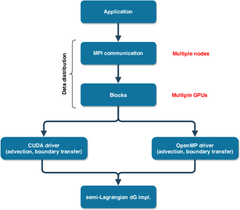
Figure 1: An overview of the structure of the SLDG code used in this paper.

The main computational effort in the present algorithm is performing the advections and computing the density/physical invariants. For the former, as mentioned above, a semi-Lagrangian discontinuous Galerkin scheme is used. The degrees of freedom are given by function values $u_{ij}^{m}\approx u^{m}(x_{i-1/2}+\xi_{j})$, where $i$ is the cell-index, which runs from $0$ to $n_{C}$, $x_{i-1/2}$ is the left cell interface, and $\xi_{j}$ is the $j$th Gauss–Legendre node scaled to the interval $[0,h]$, where $h$ is the cell size. The indices $j$ run from $0$ to $o-1$, where $o$ is the order of the method. For simplicity we only consider the one-dimensional case here. More detailed information can be found in [8]. To perform the $L^{2}$ projection at the heart of the algorithm only data from at most two adjacent cells is required. We denote the index of these two cells by $i^{\star}$ and $i^{\star}+1$, respectively. The resulting numerical scheme then computes $u_{ij}^{m+1}$ from $u_{ij}^{m}$ as follows

$$u_{ij}^{m+1}=\sum_{l}A_{jl}u_{i^{\star}l}^{m}+\sum_{j}B_{jl}u_{i^{\star}+1;l}^{m},$$

where $A\in\mathbb{R}^{o\times o}$ and $B\in\mathbb{R}^{o\times o}$. This computation has to be done for each $i$ and $j$ and for each slice of the high-dimensional problem. The amount of memory accesses is equal to two times (one read and one write) the degrees of freedom. On the other hand, we require at least $2o$ times the degrees of freedom many arithmetic operations. Nevertheless, this is a memory bound problem on most modern hardware architectures (including GPUs). We also mention that assembling the (small) matrices $A$ and $B$ takes some time. However, this usually only requires a small part of the overall run time. Computing the density and the physical invariants is also essentially a memory bound problem. However, we note that to compute the invariants a fair amount of arithmetic operations have to be performed as well. We are required to compute the density in every time step as the electric field depends on it. We also calculate the other physical quantities (such as the electric energy, kinetic energy, total energy, mass, $L^{2}$ norm, …) in every time step. Some of those, e.g. the electric energy, are used for visualization of the solution, while others, such as the total energy, serve as a diagnostic for the numerical solution.

3 Single GPU performance and comparison with CPU

In this section we will consider the performance of a single GPU and compare it to a dual socket CPU system. We consider a NVIDIA V100 GPU (with NVLink interconnect) and a NVIDIA Titan V. Both of these GPUs are based on the Volta architecture. For comparison we will also consider the (rather outdated) NVIDIA K80. The K80 is a dual GPU board. Thus, for the results in this section we will only use one of the two GPUs that are part of the K80 package. A list of the theoretical hardware characteristics of these GPUs is given in Table 1. The main CPU system used for comparison is based on two 16 core Intel Xeon Gold 6130 CPUs operating at 2.1 GHz. More details can be found in Table 1.

		TFlops/s
		double	single		GB/s
2x Xeon Gold 6130		2.2	4.3		256
2x Xeon E5-2630 v3		0.6	1.2		59
V100		7.5	15		900
Titan V		6.9	13.8		653
0.5x K80		1.5	4.4		240
1x K80		2.9	8.7		480
GTX 1080 Ti		0.35	11.3		484
NVLink (V100)		–	–		300
PCIe 3.0 x16		–	–		16

Table 1: The main hardware characteristics, i.e. peak arithmetic performance for single and double precision and the theoretically attainable memory bandwidth, for the dual socket server system and the GPUs that are used in the numerical simulations are listed. In addition, we also state the theoretical bandwidth for NVLink (on the V100) and the theoretical bandwidth for the PCIe configuration found in our system.

All performance results given in this section will be measured in terms of achieved bandwidth. That is, we count the number of bytes we have to transfer from (read) and to (write) memory. In the Strang splitting algorithm used we have to conduct $6$ advections, which require one read of the input array and one write to the output array each (this assumes that every duplicated local memory access incurs no additional cost; i.e., that locally all data accesses are perfectly cached). In addition, we have to compute the density $\rho$ twice. Once at the middle of the time step to compute the appropriate electric field to obtain second order and once at the beginning of the time step to write the electric energy and other invariant to file. Each of those reductions requires one read of the input array. Thus, for each time step we have to access the entire data set in memory $14$ times. The total amount of memory transferred is $14\cdot N\cdot\text{sizeof(}\text{double})$, where $N$ is the number of degrees of freedom that are used in the simulation. The achieved bandwidth is then computed as follows

$$\text{achieved bandwidth}=\frac{14\cdot N\cdot\text{sizeof}(\text{double})}{t_{\text{timestep}}},$$ (1)

where $t_{\text{timestep}}$ is the average wall-time required to compute one time step. In the actual algorithm a number of additional tasks have to be done. For example, computing the electric field from the density, copying the electric field to the GPU, assembling boundary conditions and copying them to the GPU, etc. However, since those operations are usually cheap compared to operations that involve the entire data set, we neglect them for the present consideration.

In contrast to the also very common practice of stating floating point operations per second, using the achieved bandwidth to measure performance, and thus as our figure of merit, has two main advantages. First, the numerical method is memory bound (see the discussion above and the references given). Thus, stating the performance in terms of bandwidth makes it easy to compare the performance to what is theoretically possible on the underlying hardware. Second, the measure is independent of the order of the numerical method. That is, no matter if we use a second or fourth order scheme the amount of data we have to read/write only depends on the total number of degrees of freedom. In addition, the way we have defined achieved bandwidth here does not depend on whether we use a CPU, a single GPU, or multiple GPUs. The achieved bandwidth is proportional to the inverse of the wall time (this is possibly since we do not take, for example, copying boundary data between GPUs into account; this is all overhead that reduces the performance and is not considered part of the algorithm). This makes comparisons in terms of what practitioners care about, i.e. wall time, straightforward. It should, however, be noted that the achieved memory bandwidth can not be directly used to compare different numerical methods; in particular, this applies to methods with different order. In this case any advantage in achieved bandwidth would have to be contrasted to a potential decrease in accuracy. Weather a higher method or a lower order method is more effective also depends strongly on the specific problem, weather we are interested in long time behavior or not, as well as many other factors. For the semi-Lagrangian discontinuous Galerkin scheme some of those factors have been considered in [10, 9]. We refer the interested reader to these papers for more details. However, for our present goal, i.e. evaluating the efficiency of the implementation using the achieved bandwidth as the figure of merit is the appropriate approach.

We consider the integration of a four dimensional Vlasov–Poisson equations (two dimensions in physical space and two dimensions in velocity) on a single GPU/dual socket CPU system. The corresponding results are shown in Figure 2. The performance is investigated as a function of the number of degrees of freedom (on the $x$-axis) and the order $o$ of the numerical method. On the CPU the performance is at most $46$ GB/s. For the V100 GPU we observe between 355 (order 6) and 483 (order 2) GB/s. There is a significant penalty in terms of achieved bandwidth when using higher order methods. However, we should note that the 4th order method, which seems to be a good choice for many problems in practice, still achieves 470 GB/s on the V100 (and 381 GB/s on the Titan V). A simple streaming benchmark (using a call to cudaMemcpy) on the V100 gives approximately 800 GB/s (significantly less than the 900 GB/s listed by the vendor). This is the maximum a memory bound problem can achieve. Our implementation obtains approximately 60% of that value. Although, research on stencil codes has demonstrated results that are closer to this limit [31, 33, 34], given that our numerical algorithm needs significantly more floating point operations, operates in a higher dimensional setting (almost all stencil implementations consider only problems in up to three dimensions), is implemented independently of the dimension of the problem (which is not true for most stencil codes which either have a fixed dimension [31] or use code generation [33, 34]), and the fact that we include overhead specific to the Vlasov equation (in particular, the Poisson solver and the communication of boundary data) in computing the achieved bandwidth, means that we achieve excellent performance.

Overall, there is approximately a factor of $10$ speed up for the V100 compared to our dual socket CPU node. We note that the percentage of the theoretical peak performance achieved for the CPU implementation is somewhat less compared to the GPU implementation. In our opinion this is ultimately due to the simpler architecture of the GPU, which gives us the ability to more directly control data transfer (e.g. via shared memory). Generally, we also found the performance on the GPU to be more predictable. On the CPU side even some relatively minor changes could have a significant impact on performance. Moreover, although the problem is memory bound, a significant amount of arithmetic operations still has to be performed. In our experience GPUs are better able to hide the associated latency. Let us also note that the performance characteristics for the Titan V are rather similar to the V100; the code achieves between 315 (order $6$) and 429 GB/s (order $2$). The performance difference between the two platforms is between 10 and 25%, depending on the order of the method.

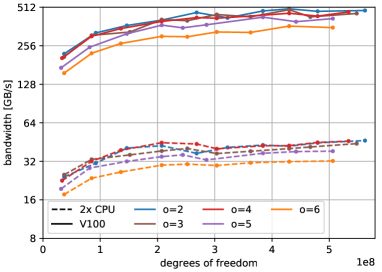
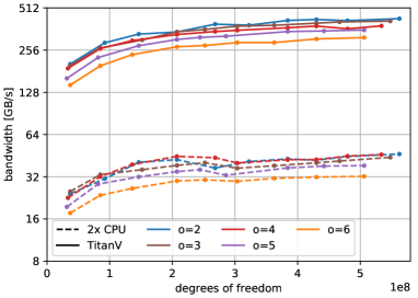
Figure 2: Single GPU and dual socket CPU performance for solving the 2+2 dimensional Vlasov–Poisson equation. The achieved bandwidth for a V100 (left) and Titan V (right) as a function of the number of degrees of freedom is shown. The simulation are performed using double precision floating point numbers.

For historical reasons and to provide further context for the present comparison, we will also consider a single GPU of the K80 package (Kepler architecture). Obviously, this is a different system and we thus use the dual socket Intel Xeon CPU E5-2630 v3 as the basis for the comparison. The results are shown in Figure 3. Here we achieve approximately 16 GB/s on the dual socket CPU system and from 60 to 76 GB/s on the GPU. Thus, we observe a speed up on the GPU of approximately a factor of $4$. The difference in performance between the V100 and the K80 is approximately a factor $6$ (the release dates of these two GPUs are approximately three years apart).

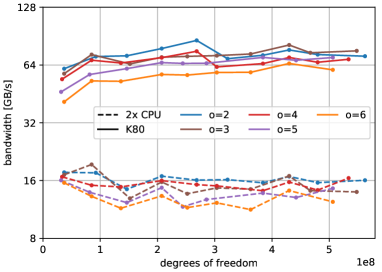
Figure 3: Single GPU and dual socket CPU performance for solving the 2+2 dimensional Vlasov–Poisson equation. The achieved bandwidth for one GPU in the K80 package is shown as a function of the number of degrees of freedom. The simulations are performed using double precision floating point numbers.

4 Multiple GPU performance

In this section we will consider simulations that run on multiple GPUs. In this context the entire domain is equally distributed along the two directions in velocity. Each GPU that takes part in the computation is thus responsible for a part of the domain. The algorithm requires an additional communication step that transfers the required boundary data between the different GPUs. If we denote the degrees of freedom stored on a single GPU in the $x_{1}$, $x_{2}$, $v_{1}$, and $v_{2}$ directions by $n_{x_{1}}$, $n_{x_{2}}$, $n_{v_{1}}$, and $n_{v_{2}}$, respectively, the total number of degrees of freedom per GPU is $N_{GPU}=n_{x_{1}}n_{x_{{}_{2}}}n_{v_{1}}n_{v_{2}}$. This is also the amount of degrees of freedom we have to transfer to and from memory in every advection step. On the other hand, the amount of boundary data we have to transfer is significantly smaller. For example, for the advection in the $x$-direction we have to transfer $Con_{x_{2}}n_{v_{1}}n_{v_{2}}$ degrees of freedom from each GPU to each other GPU, where $C$ is the CFL number and $o$ is the order of the method used, . Thus, the data that has to be transferred is smaller than the number of memory accesses by a factor of $Co/n_{x_{1}}$. However, we also have to realize that the bandwidth available is significantly reduced. In particular, this is true for the systems with PCIe, as is illustrated in Table 1.

In this section we consider performance in the multi-GPU, but single node setting. This is interesting as for both large supercomputers and desktop workstations it is very common to have multiple GPUs available on each node. These GPUs are then connected either via NVLink (this is an option for the V100) or using PCIe. Thus, one main goal of this section is to investigate the performance implications of NVLink for our code. The main utility of having a faster interconnect, in the present context, is to speed up the transfer of the boundary data.Walker

Our setup consists of four GPUs of each type on the same node. The V100 GPUs have an NVLink interconnect, while the Titan V are connected via PCIe. The results for the V100 and Titan V are shown in Figure 4. The performance observed ranges from 1165 GB/s to 1745 GB/s for the V100 and from 543 to 1094 GB/s for the Titan V. The fourth order method achieves 1602 GB/s on the four V100 and 747 GB/s on the four Titan V. Thus, we conclude that the availability of NVLink gives a significant boost in performance, approximately a factor of two. The speed up compared to a single GPU is also rather good for the V100 configuration, approximately a factor of $3.5$. For the Titan V on the other hand, we only observe slightly more than a factor of two. Thus, there is a significant discrepancy in performance between the V100 and Titan V configurations.; approximately a factor of two for the fourth order method.

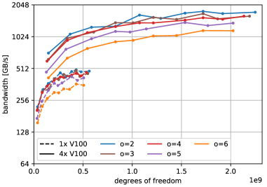
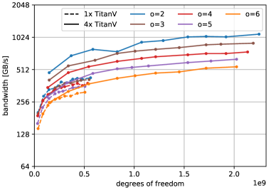
Figure 4: Performance of four GPUs on a single node for solving the 2+2 dimensional Vlasov–Poisson equation. The achieved bandwidth for four V100 (left) and four Titan V (right) as a function of the number of degrees of freedom is shown. The simulation are performed using double precision floating point numbers. For comparison the results for a single GPU of the same type are shown as well.

This is a good time to pause and investigate the performance characteristics of the code in more detail. To do that we will consider Figure 5. There the wall time for different parts of the program is shown as a bar chart. We are particularly interested in the disparity in performance for schemes of different order. We will discuss this both for the single and the multi-GPU configuration. Figure 5 divides the execution of the program into the following parts advection x (computing the translation in the direction of space variables), advection v (computing the translation in the direction of velocity variables), compute rho (computing the density, required for computing the electric field, and some physical invariants), poisson (computing the electric field by solving a Poisson equation), boundary (collecting the boundary data and all communication that is necessary), and remainder (everything that has not been accounted for in the listed categories). Before proceeding, let us note that computing the advection in the velocity directions is actually more expensive than computing the advection in the space directions. The bars denote the entire run time and, due to the the Strang splitting, the advections in the space directions are called twice as often as the corresponding advections in the velocity direction.

We clearly see that although there is some additional cost to compute the advections for higher order schemes, this is only part of the performance difference. In the multi-GPU setting the time it takes to transfer boundary data from one GPU to its neighboring GPU is also very important. This scales unfavorably with the order of the method as the algorithm has to send a fixed number of cells. For higher order methods each cell contains more degrees of freedom and thus a larger amount of data needs to be transferred. This is, of course, particularly an issue for the slower interconnect on the Titan V and we indeed see from 5 that for four Titan V and $o=6$ approximately half of the run time of the algorithm is spend in transferring boundary data. However, we should note that higher order methods are also more accurate (for the same number of degrees of freedom), which at least to some extent compensates for this overhead.

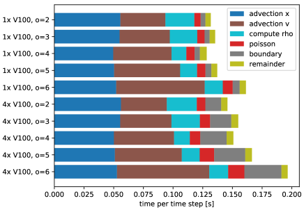
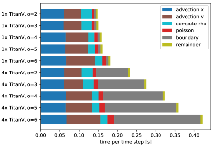
Figure 5: The wall time for different parts of the Vlasov solver are shown. Results are given for single GPU and multi-GPU configurations (V100 on the left and Titan V on the right) and as a function of the order $o$ of the numerical scheme. The degrees of freedom on each GPU is held constant (strong scaling). That is, the overall problem size is proportional to the number of GPUs employed (approximately $0.5\cdot 10^{9}$ degrees of freedom for the single GPU setup and $2\cdot 10^{9}$ degrees of freedom for the four GPU setup). Thus, ideally the time per time step going from a single to four GPUs would remain constant. The legend is explained in more detail in the main text.

All configurations so far have used peer-to-peer transfer to directly copy boundary data from one GPU to another. We will now investigate how much performance improvement this approach yields compared to doing the boundary data transfer via the host. There is not really a point in doing this for the present application, as peer-to-peer transfer is already implemented and is available on both the V100 and Titan V. Nevertheless, using host transfer is somewhat simpler and in some settings it could be questioned if the additional complexity in the code is justified. Moreover, it is interesting to see how much gain in performance we actually obtain by such an implementation. The results are shown in Figure 4. The performance difference in our code is quite significant. For example, for the fourth order method the performance of the V100 drops from approximately 1602 GB/s (peer-to-peer) to approximately 726 GB/s (host transfer). For the Titan V the difference is somewhat smaller, as one might suspect. But even in this case a significant fraction of performance is lost.

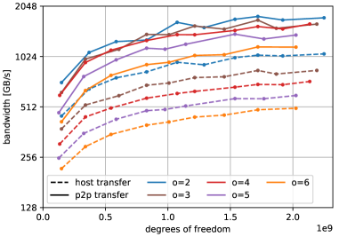
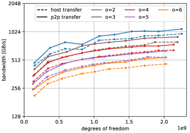
Figure 6: Comparison of peer-to-peer data transfer and data transfer via the host for the 2+2 dimensional Vlasov–Poisson equation. The achieved bandwidth for four V100 (left) and four Titan V (right) as a function of the number of degrees of freedom is shown. The simulation are performed using double precision floating point numbers.

As before, we also consider the K80. Here we only scale up to the 2 GPUs found in that package. The corresponding results are shown in Figure 7. We observe approximately a factor of $1.5$-$1.7$ improvement in performance by going from a single GPU to two GPUs. Let us note that even though the two GPUs in the K80 package are connected using PCIe, this is completely done within the package provided by the vendor.

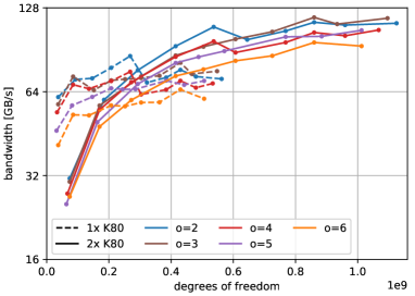
Figure 7: Performance of the two GPUs in the K80 package for solving the 2+2 dimensional Vlasov–Poisson equation. The achieved bandwidth as a function of the number of degrees of freedom is shown. The simulation are performed using double precision floating point numbers. For comparison the results for a single GPU are shown as well.

5 Single precision performance

Since many scientific applications (stencil codes, sparse matrix operations, the semi-Lagrangian discontinuous Galerkin algorithm considered here, etc.) are now memory bound on virtually all modern hardware architectures, reducing the amount of memory that is required to run a simulation is beneficial in two ways. First, it increases performance by reducing the amount of data that have to be read/written to/from memory. Second, reducing the overall amount of memory can be quite valuable on more memory constraint platforms. such as GPUs. This enables us to run a larger simulation on each GPU. Moreover, consumer level GPUs, which are significantly less expensive, have much better single precision than double precision performance (we will discuss this more in section 6). Thus, single and mixed precision computation have become an important topic of research in the last decade. In fact, for the Vlasov equation a mixed precision algorithm has been proposed in [7]. The present code supports simulation using both double and single precision. In particular, care has been taken that no unnecessary round-off errors are introduced. This is less an issue for the transport part of the algorithm. Computing a number of physical quantities, on the other hand, is more problematic as those requires a reduction over the entire data set. In our implementation double precision accumulators are used on the CPU. This has only a negligible impact on performance. On the GPU a natural way to implement reduction is in a hierarchical fashion (reduction within a single block first, then reduction within a grid, then reduction of the results on the CPU). This algorithm is less problematic with respect to round-off errors. The software package has a number of unit tests that check if the error of the implementation is reasonable.

We now consider the same configuration as in section 3, except that all data are stored as single precision floating point numbers. Equation 3 is modified in the obvious way to take this into account. The corresponding results are shown in Figure 8 (dashed lines). We observe that the achieved bandwidth for single precision computations on a single V100 is somewhat reduced; approximately 15% for the fourth order method. For the Titan V the situation is similar. Let us emphasize that even though the efficiency (as measured by the achieved bandwidth) is slightly lower, the real world performance , i.e. how many degrees of freedom can be processed in one second, is still significantly higher. For the fourth order method we observe a reduction in memory by a factor of two and, for the same number of degrees of freedom, a reduction in run time by a factor of approximately $1.7$ for the V100 and $1.8$ for the Titan V. For comparison Figure 9 (dashed lines) shows the single precision performance of a single GPU in the K80 package.

We now report single precision results on multiple GPUs, i.e. the configuration in section 4. The results for V100 and Titan V are given in Figure 8 and the corresponding results for the K80 are given in Figure 9. For the V100 the results are very similar to the single GPU case. That is, we observe a small reduction in efficiency but still an overall gain in performance by going from double to single precision. For the Titan V the difference in efficiency between single and double precision is very small.

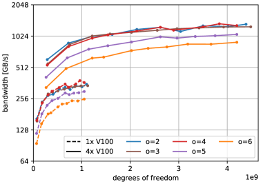
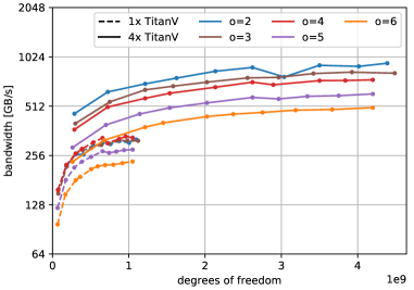
Figure 8: Performance of a single and four GPUs on one node for solving the 2+2 dimensional Vlasov–Poisson equation. The achieved bandwidth for the V100 (left) and the Titan V (right) GPUs as a function of the number of degrees of freedom is shown. The simulation are performed using single precision floating point numbers. For comparison the results for a single GPU of the same type are shown as well.

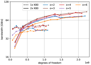
Figure 9: Performance of the two GPUs in the K80 package for solving the 2+2 dimensional Vlasov–Poisson equation. The achieved bandwidth as a function of the number of degrees of freedom is shown. The simulation are performed using single precision floating point numbers. For comparison the results for a single GPU are shown as well.

6 Performance of consumer level GPUs

Consumer GPUs, i.e. those GPUs that are are primarily marketed towards gaming applications, have one decisive advantage; namely, their low price. Their main drawback for scientific computation is the lack of good performance for double precision computations. Double precision computations have long been considered the gold standard for doing scientific computing. However, due to the appearance of hardware architectures where single precision computations are advantageous, significant research into single and mixed precision algorithms has been conducted. Consumer GPUs also do not feature error correcting (ECC) memory nor do they offer NVLink support. Other than that, the specification of those GPUs are often almost on par with the Tesla (and Titan V) cards, the latter of which are more marketed towards the scientific computing community. Because of this, many fields within scientific computing that do not require strong double precision performance or very fast interconnects, such as machine learning or molecular dynamics, have embraced consumer level GPUs.

The goal of the present section is to investigate the performance of such a consumer level GPU for our application. As an example, we have chosen the GTX 1080 Ti; see Table 1 for more details. The corresponding results are shown in Figure 10. We observe that the difference in performance for this GPU between single and double precision performance is not as large as one might expect. However, remember that we have a memory bound problem and thus the inability of the GTX 1080 Ti to do double precision operations natively has not a drastic effect on performance. The difference for the 4th order scheme, for example, is approximately 30% in terms of efficiency (i.e. approximately a factor of $2.6$ between single and double precision simulations). Note, however, that even in the single precision case the GTX 1080 Ti achieves only a fraction of the performance compared to the V100 or Titan V (132 GB/s vs 411 GB/s and 350 GB/s, respectively, for the fourth order method). In the multiple GPU setting, 6 GTX 1080 Ti are able to achieve a combined single precision bandwidth of 612 GB/s. This is just short of twice the performance of a Titan V.

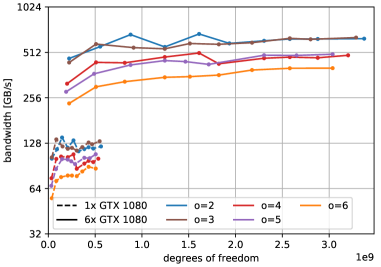
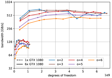
Figure 10: Performance of six GTX 1080 Ti GPUs on a single node for solving the 2+2 dimensional Vlasov–Poisson equation. The achieved bandwidth is shown as a function of the number of degrees of freedom. The simulation are performed using double precision (left) and single precision (right) floating point numbers. For comparison the results for a single GPU of the same type are shown as well.

In Figure 11 we investigate the performance normalized to procurement cost. We see that for both double and single precision the GTX 1080 Ti cards have an advantage here. Despite this, the V100 and TitanV perform very similar according to this this metric. The overall advantage of any GPU solution compared to the dual socket Xeon Gold 6130 node is approximately a factor of $6$ to $7$.

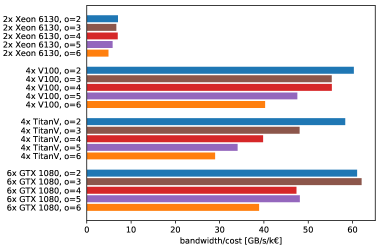
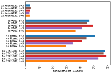
Figure 11: Performance normalized to cost for solving the 2+2 dimensional Vlasov–Poisson equation. The achieved bandwidth per 1000 € of procurement cost on a single node is shown. The simulation are performed using double precision (left) and single precision (right) floating point numbers.

7 Performance in 1+3d and 2+3d

As described in the introduction, our implementation is able to handle arbitrary dimensions, in both the $x$ and $v$-direction, within the same code base. This is, in particular, an advantage if good performance for different configurations can be achieved. In this case a single code base is sufficient to treat all the different configurations and no additional code to specifically optimize certain configurations has to be written. This simplifies the maintenance of the software package enormously. To demonstrate that this is indeed the case for SLDG we will consider 1+3 dimensional (i.e. 1 dimension of space and 3 dimensions of velocity) and 2+3 dimensional (i.e. 2 dimensions in space and 3 dimensions in velocity) simulation in this section. For brevity, we will only present results for double precision computations and V100 GPUs here. However, we emphasize that there are no surprises when looking at the performance of the other GPUs considered in this paper.

Let us start with the 1+3 dimensional case. The corresponding results for the configuration from sections 3 and 4 are shown in Figure 12. In this setting the performance is very similar to the 2+2 dimensional case considered so far. For example, for the fourth order scheme we achieve a bandwidth of approximately 424 GB/s for a single V100 and 1584 for four V100 connected via NVLink. We note that the difference between the schemes with different order is less pronounced; even the sixth order scheme achieves 1265 GB/s on four V100 GPUs. Before proceeding let us note that the performance on the CPU is very similar to what has been observed in section 3 for the 2+2 dimensional case. We achieve approximately 40 GB/s. Also in this case the spread between the schemes of different order is significantly reduced.

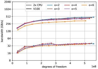
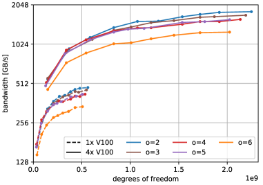
Figure 12: Performance of V100 GPUs for solving the 1+3 dimensional Vlasov–Poisson equation. The achieved bandwidth for a single V100 (left) and four V100 (right) is shown as a function of the number of degrees of freedom. The simulation are performed using double precision floating point numbers.

We now consider the 2+3 dimensional case. Thus, we simulate a five dimensional problem. The obtained results are shown in Figure 13. We remark that the achieved bandwidth is slightly reduced compared to the 2+2 dimensional case. For example, for the fourth order method a single V100 achieves 307 GB/s and four V100 achieve 1077 GB/s. A similar reduction in performance can be observed for the CPU and thus, overall, the difference between the CPU and the single GPU implementation is still approximately a factor of $10$.

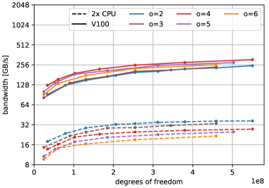
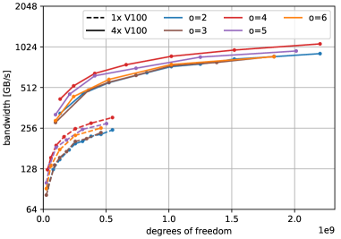
Figure 13: Performance of V100 GPUs for solving the 2+3 dimensional Vlasov–Poisson equation. The achieved bandwidth for a single V100 (left) and four V100 (right) is shown as a function of the number of degrees of freedom. The simulation are performed using double precision floating point numbers.

8 Numerical simulation & validation

In this section we will discuss the steps we have taken to validate our code. In SLDG we make use of a range of automated tests. This includes unit testing the components and algorithms that make up the software package (using Boost.Test). In particular, automatic tests check the convergence rate of all numerical algorithms involved and test their accuracy, in cases where analytic solutions can be constructed. In addition, we test the results of numerical simulations for the complete Vlasov equation. For the latter we make use of analytic properties that are available in certain situations. For example, we have a test where a multi-dimensional linear Landau damping simulation is conducted. Since the analytic decay rate (as a function of the wave number of the initial perturbation) is known, we use this to check the output of the numerical simulation. We also use properties of the numerical algorithm, such as mass and momentum conservation, to further verify the code. For all the numerical simulations that have been conducted in order to obtain the results presented in sections 3-7 we automatically check that all runs give the same results (within the approximation error).

Finally, we compare the output of numerical simulations, for which no analytic properties are available, to known results from the literature. We will present one such simulation here. Namely, a four-dimensional two-stream instability given by the initial data

$$f(0,x_{1},x_{2},v_{1},v_{2}) =(1+\epsilon(\cos(kx_{1})+\cos(kx_{2})))f^{\text{eq}}(v_{1},v_{2})$$ (2)

with

$$f^{\text{eq}}(v_{1},v_{2})=\frac{1}{8\pi}\left(\mathrm{e}^{-(v_{1}-v_{0})^{2}/2}+\mathrm{e}^{-(v_{1}+v_{0})^{2}/2}\right)\left(\mathrm{e}^{-(v_{2}-v_{0})^{2}/2}+\mathrm{e}^{-(v_{2}+v_{0})^{2}/2}\right),$$

where $\epsilon=10^{-3}$, $k=0.2$, and $v_{0}=2.4$. The computational domain is $[0,10\pi]^{2}\times[-6,6]^{2}$. The time evolution of the electric field and some snapshots of the density function are shown in Figure 14. We remark that these results agree well with what has been reported in the literature (see, for example, [24, 1]). Figure 14 shows both single and double precision results, which are almost indistinguishable in the plots. The difference in the distribution function (measured in the infinity norm), the electric field (measured in the infinity norm), and the relative difference in electric energy are below $2\cdot 10^{-4}$. In addition, we show the time evolution of the physical invariants mass, energy, and $L^{2}$ norm in Figure 15. We observe that for both energy as well as the $L^{2}$ norm the difference between double and single precision result is very small.

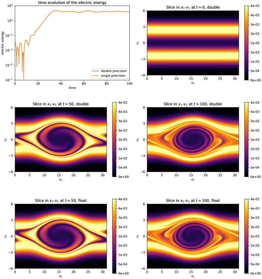
Figure 14: Numerical simulation of the two-stream instability given by equation (2). On the top-left the time evolution of the electric field is shown (note that the double and single precision results almost overlap). The remaining plots are $x_{1}-v_{1}$ slices of the density function $f$ at time $t=0$ (top-right), $t=50$ (middle-left for double precision and bottom-left for the single precision simulation), and $t=100$ (middle-right for double precision and bottom-right for the single precision simulation). The simulation is conducted on a grid of size $60^{4}\cdot 4^{4}$. That is, in each coordinate direction $60$ cells, each with $o=4$ degrees of freedom (i.e. the fourth order semi-Lagrangian discontinuous Galerkin scheme) are used.

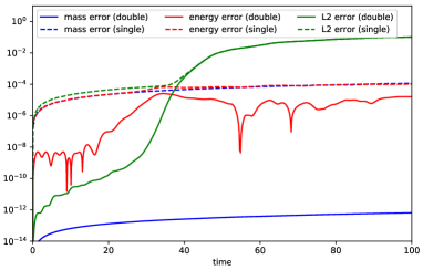
Figure 15: Numerical simulation of the two-stream instability given by equation (2). The time evolution of the relative error in mass, energy, and $L^{2}$ norm is shown. The simulation is conducted on a grid of size $60^{4}\cdot 4^{4}$. That is, in each coordinate direction $60$ cells, each with $o=4$ degrees of freedom (i.e. the fourth order semi-Lagrangian discontinuous Galerkin scheme) are used.

9 Conclusion

We have shown that the dimension independent semi-Lagrangian Vlasov solver SLDG can achieve excellent performance on systems with single and multiple GPUs. In fact, the single node GPU performance (i.e. 4 V100 GPUs on the same node compared to the dual socket CPU system) shows a speed up of approximately a factor of $35$ compared to a dual socket CPU node. We further emphasize that the Titan V also shows excellent performance characteristics. The main performance bottleneck for the Titan V in the multi-GPU setup is the absence of a fast interconnect (such as NVLink).

Although there are some variations, the observed performance is rather predictable across 2+2 dimensional, 1+3 dimensional, and 2+3 dimensional Vlasov simulations. This is a good validation of our approach to develop a dimension independent code. It is also interesting to note that higher order methods are less efficient than lower order methods. One might be tempted to blame this on the increased computational burden. However, as discussed, the increased data transfer plays an even larger role. This is particularly true for GPUs without a fast interconnect. Performance on the GTX 1080 Ti is rather disappointing giving the theoretical memory bandwidth of those GPUs. However, on a pure performance per cost basis consumer cards are still winning out. It is interesting to note that this is true for both single and double precision computations. That is, there is only a modest performance penalty for the double precision implementation on the GTX 1080 Ti.

The current version of the SLDG code can be found at https://bitbucket.org/leinkemmer/sldg. The code can be freely used under the terms of the MIT license.

References

- [1] Y. Barsamian, J. Bernier, S.A. Hirstoaga, and M. Mehrenberger. Verification of 2D 2D and two-species Vlasov-Poisson solvers. ESAIM: Proceedings and Surveys, 63:78–108, 2018.
- [2] M. Brunetti, F. Califano, and F. Pegoraro. Asymptotic evolution of nonlinear Landau damping. Phys. Rev. E, 62(3):4109, 2000.
- [3] M. Bussmann, H. Burau, T. E. Cowan, A. Debus, A. Huebl, G. Juckeland, T. Kluge, W. E. Nagel, R. Pausch, F. Schmitt, U. Schramm, J. Schuchart, and R. Widera. Radiative Signatures of the Relativistic Kelvin-Helmholtz Instability. In Proceedings of the International Conference on High Performance Computing, Networking, Storage and Analysis, SC ’13, pages 5:1–5:12, New York, NY, USA, 2013. ACM.
- [4] F. Califano, L. Galeotti, and A. Mangeney. The Vlasov-Poisson model and the validity of a numerical approach. Phys. Plasmas, 13(8):082102, 2006.
- [5] A. Crestetto and P. Helluy. Resolution of the Vlasov-Maxwell system by PIC Discontinuous Galerkin method on GPU with OpenCL. In ESAIM: Proceedings, volume 38, pages 257–274. EDP Sciences, 2012.
- [6] N. Crouseilles, M. Mehrenberger, and F. Vecil. Discontinuous Galerkin semi-Lagrangian method for Vlasov-Poisson. In ESAIM: Proceedings, volume 32, pages 211–230. EDP Sciences, 2011.
- [7] L. Einkemmer. A mixed precision semi-Lagrangian algorithm and its performance on accelerators. In High Performance Computing and Simulation (HPCS), International Conference on, 2016.
- [8] L. Einkemmer. High performance computing aspects of a dimension independent semi-Lagrangian discontinuous Galerkin code. Comput. Phys. Commun., 202:326–336, 2016.
- [9] L. Einkemmer. A study on conserving invariants of the Vlasov equation in semi-Lagrangian computer simulations. J. Plasma Phys., 83(2), 2017.
- [10] L. Einkemmer. A performance comparison of semi-Lagrangian discontinuous Galerkin and spline based Vlasov solvers in four dimensions. J. Comput. Phys., 376:937–951, 2019.
- [11] L. Einkemmer and C. Lubich. A low-rank projector-splitting integrator for the Vlasov–Poisson equation. SIAM J. Sci. Comput., 40:B1330–B1360, 2018.
- [12] L. Einkemmer and C. Lubich. A quasi-conservative dynamical low-rank algorithm for the Vlasov equation. SIAM J. Sci. Comput., 41(5):B1061–B1081, 2019.
- [13] L. Einkemmer and A. Ostermann. Convergence analysis of a discontinuous Galerkin/Strang splitting approximation for the Vlasov–Poisson equations. SIAM J. Numer. Anal., 52(2):757–778, 2014.
- [14] L. Einkemmer, A. Ostermann, and C. Piazzola. A low-rank projector-splitting integrator for the Vlasov–Maxwell equations with divergence correction. arXiv:1902.00424, 2019.
- [15] E. Fijalkow. Numerical solution to the Vlasov equation: The 1D code. Comput. Phys. Commun., 116(2):329–335, 1999.
- [16] F. Filbet and E. Sonnendrücker. Comparison of Eulerian Vlasov Solvers. Comput. Phys. Commun., 150:247–266, 2003.
- [17] French Atomic Energy Commision and University of Strasbourg and Max-Planck-Institut fÃŒr Plasmaphysik (IPP). SeLaLib. http://selalib.gforge.inria.fr/.
- [18] L. Galeotti and F. Califano. Asymptotic Evolution of Weakly Collisional Vlasov-Poisson Plasmas. Phys. Rev. Lett., 95:015002, 2005.
- [19] W. Guo and Y. Cheng. A sparse grid discontinuous Galerkin method for high-dimensional transport equations and its application to kinetic simulation. SIAM J. Sci. Comput., 38(6):3381–3409, 2016.
- [20] J.A.F. Hittinger and J.W. Banks. Block-structured adaptive mesh refinement algorithms for Vlasov simulation. J. Comput. Phys., 241:118–140, 2013.
- [21] M. Horowitz, E. Alon, D. Patil, S. Naffziger, R. Kumar, and K. Bernstein. Scaling, power, and the future of CMOS. In IEEE InternationalElectron Devices Meeting. IEEE, 2005.
- [22] D. Jarema, H. Bungartz, T. Görler, F. Jenko, T. Neckel, and D. Told. Block-structured grids for Eulerian gyrokinetic simulations. Comput. Phys. Commun., 198:105–117, 2016.
- [23] D. Jarema, H. Bungartz, T. Görler, F. Jenko, T. Neckel, and D. Told. Block-structured grids in full velocity space for Eulerian gyrokinetic simulations. Comput. Phys. Commun., 215:49–62, 2017.
- [24] K. Kormann. A semi-Lagrangian Vlasov solver in tensor train format. SIAM J. Sci. Comput., 37:613–632, 2015.
- [25] K. Kormann and E. Sonnendrücker. Sparse grids for the Vlasov–Poisson equation. Sparse Grids Appl., pages 163–190, 2014.
- [26] G. Manfredi. Long-time behavior of nonlinear Landau damping. Phys. Rev. Lett., 79(15):2815, 1997.
- [27] A. Mangeney, F. Califano, C. Cavazzoni, and P. Travnicek. A numerical scheme for the integration of the Vlasov–Maxwell system of equations. J. Comput. Phys., 179(2):495–538, 2002.
- [28] M. Mehrenberger, C. Steiner, L. Marradi, N. Crouseilles, E. Sonnendrücker, and B. Afeyan. Vlasov on GPU (VOG project). In ESAIM: Proceedings, volume 43, pages 37–58. EDP Sciences, 2013.
- [29] A. Miyoshi, C. Lefurgy, E. Van Hensbergen, R. Rajamony, and R. Rajkumar. Critical power slope: understanding the runtime effects of frequency scaling. In Proceedings of the 16th International Conference on Supercomputing, pages 35–44, 2002.
- [30] M. Palmroth, U. Ganse, Y. Pfau-Kempf, M. Battarbee, L. Turc, T. Brito, M. Grandin, S. Hoilijoki, A. Sandroos, , and S. von Alfthan. Vlasov methods in space physics and astrophysics. Living Rev. Comput. Astrophys., 4(1), 2018.
- [31] I.S. Pershin, V.D. Levchenko, and A.Y. Perepelkina. Performance Limits Study of Stencil Codes on Modern GPGPUs. Supercomputing Frontiers and Innovations, 6(2):86–101, 2019.
- [32] J.M. Qiu and C.W. Shu. Positivity preserving semi-Lagrangian discontinuous Galerkin formulation: theoretical analysis and application to the Vlasov–Poisson system. J. Comput. Phys., 230(23):8386–8409, 2011.
- [33] P.S. Rawat, M. Vaidya, A. Sukumaran-Rajam, M. Ravishankar, V. Grover, A. Rountev, L. Pouchet, and P. Sadayappan. Domain-specific optimization and generation of high-performance GPU code for stencil computations. Proceedings of the IEEE, 106(11):1902–1920, 2018.
- [34] V.H.M. Rodrigues, L. Cavalcante, M.B. Pereira, F. Luporini, I. Reguly, G. Gorman, and S.X. de Souza. GPU Support for Automatic Generation of Finite-Differences Stencil Kernels. arXiv preprint, arXiv:1912.00695, 2019.
- [35] F. Rossi, P. Londrillo, A. Sgattoni, S. Sinigardi, and G. Turchetti. Towards robust algorithms for current deposition and dynamic load-balancing in a GPU particle in cell code. In AIP Conference Proceedings, volume 1507, pages 184–192, 2012.
- [36] J.A. Rossmanith and D.C. Seal. A positivity-preserving high-order semi-Lagrangian discontinuous Galerkin scheme for the Vlasov–Poisson equations. J. Comput. Phys., 230(16):6203–6232, 2011.
- [37] A. Sandroos, I. Honkonen, S. von Alfthan, and M. Palmroth. Multi-GPU simulations of Vlasov’s equation using Vlasiator. Parallel Comput., 39(8):306–318, 2013.
- [38] J. P. Verboncoeur. Particle simulation of plasmas: review and advances. Plasma Phys. Control. Fusion, 47(5A):A231, 2005.