Solenoidal scaling laws for compressible mixing

Abstract

Mixing of passive scalars in compressible turbulence does not obey the same classical Reynolds number scaling as its incompressible counterpart. We first show from a large database of direct numerical simulations that even the solenoidal part of the velocity field fails to follow the classical incompressible scaling when the forcing includes a substantial dilatational component. Though the dilatational effects on the flow remain significant, our main results are that both the solenoidal energy spectrum and the passive scalar spectrum scale assume incompressible forms, and that the scalar gradient aligns with the most compressive eigenvalue of the solenoidal part, provided that only the solenoidal components are used for scaling in a consistent manner. Minor modifications to this statement are also pointed out.

PACS numbers 47.27

A defining feature of turbulence is the ability to mix substances with orders of magnitude greater effectiveness than molecular mixing. The subject has been studied extensively Sreenivasan (2018) when the mixing agent is incompressible turbulence because it is a fundamentally important problem in its own right and a good paradigm for many practical circumstances. However, there are critically important applications from astrophysics to high-speed aerodynamics in which compressibility needs to be explicitly considered. Including compressibility renders inapplicable the Reynolds number scaling laws Lele (1994); Sarkar (1995) that are used extensively in incompressible turbulence. This paper shows one successful way of incorporating compressibility explicitly. We show by three examples that the standard incompressible laws work in the compressible case by rescaling the appropriate variables.

The initial attempt to include compressibility was through a suitably defined Mach number as an additional parameter. For the ideal case of homogeneous isotropic turbulence in a cubic box with periodic boundary conditions, this Mach number, $M_{t}=u^{\prime}/\langle c\rangle$, where $u^{\prime}=\langle u_{i}^{2}\rangle^{1/2}$, $u_{i}$ being the velocity in the Cartesian direction $i$, and the angular brackets indicate a suitable average. However, as has been pointed out by Ni Ni (2016), $M_{t}$ is not adequate when the velocity field has a strong dilatational component. Indeed, DNS data with different types of large scale forcing, such as pure solenoidal forcing Jagannathan and Donzis (2016); Donzis and Jagannathan (2013); Wang et al. (2017a), homogeneous shear forcing Chen et al. (2018), dilatational forcing Wang et al. (2018, 2013) and thermal forcing Wang et al. (2019), have revealed that the dilatational flow field characteristics depend on the details of forcing, even for fixed $M_{t}$. Further progress has been made recently Donzis and John (2019) by adding yet another parameter, namely $\delta=u_{d}^{\prime}/u_{s}^{\prime}$, which is the ratio of root-mean-square (rms) dilatational to solenoidal velocity. These two components can be readily obtained for homogeneous compressible turbulence, by utilizing the Helmholtz decomposition of the velocity field, $\mathbf{u}=\mathbf{u_{s}}+\mathbf{u_{d}},$ where the solenoidal part, $\mathbf{u_{s}}$, represents vortical contribution and satisfies the incompressibility condition $\nabla\cdot\mathbf{u_{s}}=0$. The dilatational part, $\mathbf{u_{d}}$, represents the irrotational component and satisfies $\nabla\times\mathbf{u_{d}}=0$. The improved physical understanding that arises from Donzis and John (2019) can be used to assess the scaling of the passive scalars in compressible turbulence.

The data for the current work come from direct numerical simulations (DNS) of compressible Navier-Stokes equations in a periodic box yielding homogeneous and isotropic turbulence, and span the following conditions: the microscale Reynolds number $R_{\lambda}\equiv\langle\rho\rangle u^{{}^{\prime}}\lambda/\mu$, where $\langle\rho\rangle$ is the mean density, $\lambda$ is the Taylor microscale and $\mu$ the mean dynamic viscosity, ranges from 38 to 165; the turbulent Mach number, $M_{t}$, varies between 0 and about 0.6; the Schmidt number $Sc=\mu/[\langle\rho\rangle D]$, where $D$ is the diffusivity of the scalar, is unity. The forcing at low wavenumbers contains a strong dilatational component as well, with $\delta$ ranging from 0 to 7.5. Figure 1 shows the wide range of compressibility conditions covered for the scalar field in the parameter spaces of $R_{\lambda}$, $\delta$ and $M_{t}$.

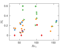
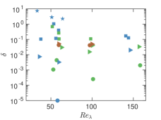
Figure 1: Parameter space of simulations for the scalar field. (a) $M_{t}$-$R_{\lambda}$ plane. Red: $\delta<10^{-3}$, Blue: $10^{-3}<\delta<10^{-2}$, Green: $10^{-2}<\delta<10^{-1}$, Orange: $10^{-1}<\delta<1$, Brown: $1<\delta<10$. (b) $\delta$-$R_{\lambda}$ plane Blue: $M_{t}<0.2$, Green: $0.2<M_{t}<0.4$, Brown: $0.4<\delta<0.7$. Symbols in all figures correspond to different percentages of dilatational forcing, $\sigma$. diamonds: incompressible simulations; circles: $\sigma=0$, triangles: $\sigma=10-30$, squares: $\sigma=30-65$, stars: $\sigma=65-100$.

The first instance of the inadequacy of incompressible scaling is the energy spectrum which, according to Kolmogorov (1941), follows the relation $E(k)=C\langle\epsilon\rangle^{2/3}k^{-5/3}$ in the inertial range, where $C$ is the Kolmogorov constant, $k$ is the wavenumber, and $\langle\epsilon\rangle$ is the mean total energy dissipation. The energy spectrum has the property that $\int_{0}^{\infty}E\left(k\right)dk=\langle u^{2}\rangle/2;\langle u^{2}\rangle=\langle u_{i}u_{i}\rangle$. In Fig. 2(a) we see that, unlike in incompressible turbulence, there is no collapse of spectral data when normalized according to Kolmogorov (1941). This is not surprising: it has been pointed out already in theories Ristorcelli (1997); Sagaut and Cambon (2008); Sarkar et al. (1991) and simulations Jagannathan and Donzis (2016); Wang et al. (2017a, 2018, 2013) that the dilatational component of energy can take on a wide range of behaviors and can depart from the classical Kolmogorov scaling.

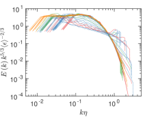
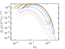
Figure 2: (a) Kolmogorov-compensated total energy spectra using total energy dissipation and Kolmogorov length scale ($\eta=\left(\mu^{3}/\langle\rho\rangle^{2}\langle\epsilon\rangle\right)^{1/4}$) Jagannathan and Donzis (2016). (b) Kolmogorov-compensated solenoidal energy spectra using total dissipation and the Kolmogorov length scale based on it. Here and in all figures to follow except the last, different colors correspond to different Reynolds numbers. Red: $R_{\lambda}<40$, blue: $40<R_{\lambda}<75$, green: $75<R_{\lambda}<115$, and orange: $115<R_{\lambda}<170$. The velocity data of this figure and of Fig. 5(a) include larger set of conditions than shown for the scalar field in Fig. 1.

As an improvement, it has been suggested that the solenoidal part of the energy spectra $\left(\nabla\cdot\mathbf{u_{s}=0}\right)$ does scale according classical Kolmogorov scaling; the basis for this claim comes from solenoidally forced DNS Jagannathan and Donzis (2016); Wang et al. (2017a). However, this result does not hold when the forcing has a strong dilatational component, as shown in Fig. 2(b), where the Kolmogorov-compensated solenoidal energy spectra $E_{s}(k)$, defined such that $\int_{0}^{\infty}E_{s}\left(k\right)dk=\langle u_{s}^{2}\rangle/2,$ does not scale when the forcing includes a dilatational part.

The second instance of this inadequacy is the scalar spectrum. In incompressible turbulence, its behavior is reasonably well understood at the phenomenological level Obukhov (1949); Corrsin (1951); Batchelor (1959); Kraichnan (1968); Watanabe and Gotoh (2004); Yeung et al. (2002); Sreenivasan (1996, 2018). For unity Schmidt number, the appropriate normalization for the passive scalars is the Obukhov-Corrsin normalization $E_{\phi}(k)=C^{\prime}\langle\epsilon_{\phi}\rangle\langle\epsilon\rangle^{-1/3}k^{-5/3}$ where $E_{\phi}$ is defined such that $\int_{0}^{\infty}E_{\phi}\left(k\right)dk=\langle\phi^{2}\rangle/2$ and $\langle\epsilon_{\phi}\rangle$ is the mean scalar dissipation; $C^{\prime}$ is the Obukhov-Corrsin constant. In Fig. 3, we plot the Obukhov-Corrsin compensated scalar spectra for all cases. There is no collapse of the data, and so compressibility appears to have a first order effect on the scalar spectra.

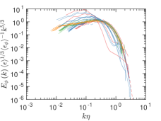
Figure 3: The Obukhov-Corrsin compensated scalar spectra using total dissipation and Kolmogorov length scale based on the total energy dissipation. No scaling is observed. Dashed line is for the incompressible case.

As a third quantity, consider the alignment of the scalar gradient with the directions of the eigenvectors of the strain field. In incompressible turbulence, the turbulent velocity field plays an important role in the stirring action of passive scalars where the different isosurfaces of the scalars are brought together Warhaft (2000); Dimotakis (2005); Sreenivasan (2018). This stirring action results in high scalar gradients across the flow field, ultimately enabling molecular diffusion to act. Batchelor’s theory Batchelor (1959), initially proposed for large Schmidt numbers, shows that the scalar gradient aligns itself with the most compressive eigenvalue. DNS studies Donzis et al. (2010) have shown that this aspect of the theory is valid, perhaps surprisingly, even for Schmidt numbers of order unity; see also Vedula et al. Vedula et al. (2001). Danish et al. Danish et al. (2016) studied this alignment for decaying compressible turbulence and found that the topology and alignment were universal for a range of Reynolds and Mach numbers, though their studies were confined to a narrow range of initial $M_{t}$ $\left(0.50-0.70\right)$ and $R_{\lambda}\left(18-24\right)$. For the wider range of compressible turbulent states considered here, in terms of $R_{\lambda}$, $M_{t}$ and $\delta$, Fig. 4 shows that the scalar gradient, $\nabla\phi=\partial\phi/\partial x_{i}$, does not align uniquely with the symmetric part of the velocity gradient tensor, $S_{ij}$, where

$$S_{ij}=\frac{1}{2}\left(\frac{\partial u_{i}}{\partial x_{j}}+\frac{\partial u_{j}}{\partial x_{i}}\right).$$

The eigenvectors of this tensor, called here $e_{\alpha}$, $e_{\beta}$, and $e_{\gamma}$, correspond respectively to the maximum, intermediate and minimum eigenvalues with $\alpha>\beta>\gamma$; incompressible turbulence is constrained by $\alpha+\beta+\gamma=0$. The previous observations by Blaisdell et al. Blaisdell et al. (1994), and more recently by Ni Ni (2016), that contributions from the dilatational field to the scalar flux are negligible compared to the solenoidal part alone, correspond to a narrow range of conditions.

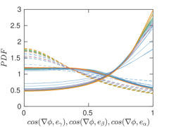
Figure 4: Alignment of scalar gradient $\left(\nabla\phi\right)$ with the eigen-directions of the $S_{ij}$, i.e. $e_{\gamma},e_{\beta},e_{\alpha}$ which correspond to the eigenvalues $\left(\gamma,\beta,\alpha\right)$ with $\gamma<\beta<\alpha$.

The discussion so far makes it clear that even the spectrum for just the solenoidal part of the velocity field does not satisfy the incompressibility scaling laws if we consider forcing with a dilatational component (see Fig. 1). Existing work Jagannathan and Donzis (2016); Wang et al. (2017a, 2011, b) which makes this claim concerns the velocity field under solenoidal forcing and decaying turbulence.

We now propose the following paradigm. Similar to the velocity field one can decompose the dissipation into solenoidal and dilatational contributions as $\langle\epsilon\rangle=\langle\epsilon_{s}\rangle+\langle\epsilon_{d}\rangle,$ where $\langle\epsilon_{s}\rangle=\langle\mu\omega_{i}\omega_{i}\rangle$, $\bm{\omega}$ being the vorticity of the fluid motion, and $\langle\epsilon_{d}\rangle=(4/3)\langle\mu\left(\partial u_{i}/\partial x_{i}\right)^{2}\rangle$ are the solenoidal and dilatational parts, respectively. Indeed, under solenoidal forcing conditions when $\delta\ll 1$ and $\langle\epsilon_{s}\rangle\approx\langle\epsilon\rangle$, we do not expect significant departures in the scaling of the solenoidal energy spectra. However, under general conditions of mixed solenoidal-dilatational forcing where $\delta$ can vary by orders of magnitude, one may expect using solenoidal variables in the compensation of the solenoidal spectra would yield better collapse. Indeed, Fig. 5(a) shows the excellent collapse of the Kolmogorov-compensated solenoidal energy spectra when both velocity and the dissipation pertain solely to the solenoidal variables. The solenoidal Kolmogorov length scale is defined Jagannathan and Donzis (2016) as $\eta_{s}=(\langle\mu\rangle^{3}/\langle\rho\rangle^{2}\langle\epsilon_{s}\rangle)^{1/4}$.

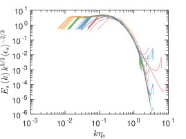
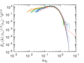
Figure 5: Kolmogorov-compensated solenoidal energy spectra (a) and Obukhov-Corrsin compensated scalar spectra (b) using solenoidal dissipation,$\langle\epsilon_{s}\rangle$ and solenoidal Kolmogorov length scale, $\eta_{s}$. Dashed line in the bottom figure is for the incompressible case.

In Fig. 5(b), we plot the Obukhov-Corrsin compensated scalar spectrum using just the solenoidal part of the velocity field. A robust collapse occurs for scalar spectra under a wide range of conditions and the spectra look similar to the incompressible case. This suggests that even at really high levels of dilatational content in the flow field, the interaction between the passive scalars and solenoidal velocity field is universal. The implication is that the cascade process in which the large scales of the passive scalar are broken down to smaller scales is independent of compressibility. Thus classical scaling laws, when modified by suitable rescaling, obey the same incompressible turbulence models in highly compressible flows, even when the dilatational part is quite strong.

We now come to the orientation of the scalar gradient with respect to the velocity strain field. Following the observations above, we assess the effect of the solenoidal component of the tensor, $S^{s}_{ij}$. In particular, we examine the statistics of the normalized eigenvalues ($\beta_{s}$) Vedula et al. (2001) given by $\widehat{\beta}_{s}={\sqrt{6}\beta_{s}}\big{/}{\sqrt{\alpha_{s}^{2}+\beta_{s}^{2}+\gamma_{s}^{2}}}$, such that $-1\leq\widehat{\beta}_{s}\leq 1$.

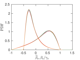
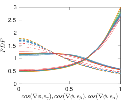
Figure 6: (a) Normalized eigenvalues of the solenoidal symmetric velocity gradient tensor, $S^{s}_{ij}$: i) $\widehat{\beta}_{s}=\sqrt{6}\beta_{s}/\sqrt{\alpha_{s}^{2}+\beta_{s}^{2}+\gamma_{s}^{2}}$; ii) $\beta_{s}/\gamma_{s}$. (b) Alignment of scalar gradient $\left(\nabla\phi\right)$ with $e_{\gamma},e_{\beta},e_{\alpha}$, the eigenvectors of $S^{s}_{ij}$.

In Fig. 6(a) is plotted the probability density function (PDF) of $\widehat{\beta}_{s}$ for a wide range of compressibility conditions. Excellent collapse is observed (curve (i)), indicating that the ratio of the PDF of the eigenvalues is unaffected by compressibility. Similar universal behavior is observed for the ratio of $\beta_{s}/\gamma_{s}$ shown as curve (ii) in the same figure. We also note that the maximum probable value of $\beta_{s}/\gamma_{s}$ is approximately $0.28$ which corresponds to the ratio of $\gamma_{s}/\beta_{s}=3.7$, close to the situation suggested for incompressible turbulence Ashurst et al. (1987) and consistent with results for solenoidal forcing Wang et al. (2012). This feature suggests that, while compressibility may change the solenoidal field itself, it does not alter its mixing capability and would remain as efficient as incompressible turbulence.

Figure 6(b) plots the alignment of the scalar gradient with the solenoidal frame of reference. One finds that the behavior of the scalar gradient is very similar to that of incompressible turbulence Vedula et al. (2001), with a high probability for the scalar gradient to align with the most compressive direction. There are, however, some weak compressibility effects. To understand them qualitatively, we show in Fig. 7 the PDF values for $\cos\left(\nabla\phi,e_{\gamma}\right)\in[0.995,1]$—that is, when the two vectors are almost perfectly aligned—as a function of turbulent Mach number, $M_{t}$. The figure shows that $R_{\lambda}$ is the major effect, though a weaker decreasing trend with $M_{t}$ is also seen. In order to completely understand compressible turbulent mixing, one has to include these secondary compressibility effects on the fine scale structure of turbulence.

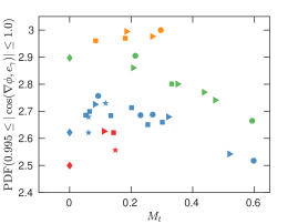
Figure 7: (a) Probability of scalar gradient $\left(\nabla\phi\right)$ being perfectly aligned with the eigendirection $e_{\gamma}$ corresponding to the most compressive eigenvalue. Symbols in the figure correspond to different percentages of dilatational forcing, $\sigma$: incompressible simulations (diamons), $\sigma=0$ (circles), 10-30 (triangles), 30-65 (squares), and 65-100 (stars).

\begin{picture}(0.0,0.0)\end{picture}

In summary, using high fidelity DNS data, we have shown that the interaction between passive scalar and solenoidal velocity field is universal under a wide range of compressibility conditions, for both the velocity and the scalar field, if both the velocity field and the energy dissipation are taken from the solenoidal part of the velocity.

References

- Sreenivasan (2018) K. R. Sreenivasan, “Turbulent mixing: A perspective,” Proc. Natl. Acad. Sci. USA (2018), 10.1073/pnas.1800463115.
- Lele (1994) S. K. Lele, “Compressibility effects on turbulence,” Annu. Rev. Fluid Mech. 26, 211–254 (1994).
- Sarkar (1995) S. Sarkar, “The stabilizing effect of compressibility in turbulent shear flow,” J. Fluid Mech. 282, 163–186 (1995).
- Ni (2016) Q. Ni, “Compressible turbulent mixing: Effects of compressibility,” Phys. Rev. E 93, 043116 (2016).
- Jagannathan and Donzis (2016) S. Jagannathan and D. A. Donzis, “Reynolds and Mach number scaling in solenoidally-forced compressible turbulence using high-resolution direct numerical simulations,” J. Fluid Mech. 789, 669–707 (2016).
- Donzis and Jagannathan (2013) D. A. Donzis and S. Jagannathan, “Fluctuations of thermodynamic variables in stationary compressible turbulence,” J. Fluid Mech. 733, 221–244 (2013).
- Wang et al. (2017a) J. Wang, T. Gotoh, and T. Watanabe, “Spectra and statistics in compressible isotropic turbulence,” Phys. Rev. Fluids 2, 013403 (2017a).
- Chen et al. (2018) S. Chen, J. Wang, H. Li, M. Wan, and S. Chen, “Spectra and mach number scaling in compressible homogeneous shear turbulence,” Phys. Fluids 30, 065109 (2018).
- Wang et al. (2018) J. Wang, M. Wan, S. Chen, C. Xie, and S. Chen, “Effect of shock waves on the statistics and scaling in compressible isotropic turbulence,” Phys. Rev. E 97, 043108 (2018).
- Wang et al. (2013) J. Wang, Y. Yang, Y. Shi, Z. Xiao, X. T. He, and S. Chen, “Statistics and structures of pressure and density in compressible isotropic turbulence,” J. Turbulence 14, 21–37 (2013), https://doi.org/10.1080/14685248.2013.831989 .
- Wang et al. (2019) J. Wang, M. Wan, S. Chen, C. Xie, L-P. Wang, and S. Chen, “Cascades of temperature and entropy fluctuations in compressible turbulence,” J. Fluid Mech. 867, 195 215 (2019).
- Donzis and John (2019) D.A Donzis and J. P. John, “Universality and scaling in compressible turbulence,” arXiv , 2771833 (2019).
- Kolmogorov (1941) A. N. Kolmogorov, “Local structure of turbulence in an incompressible fluid for very large Reynolds numbers,” Dokl. Akad. Nauk. SSSR 30, 299–303 (1941).
- Ristorcelli (1997) J. R. Ristorcelli, “A pseudo-sound constitutive relationship for the dilatational covariances in compressible turbulence,” J. Fluid Mech. 347, 37–70 (1997).
- Sagaut and Cambon (2008) P. Sagaut and C. Cambon, Homogeneous Turbulence Dynamics (Cambridge University Press, Cambridge, 2008).
- Sarkar et al. (1991) S. Sarkar, G. Erlebacher, M. Y. Hussaini, and H. O. Kreiss, “The analysis and modelling of dilatational terms in compressible turbulence,” J. Fluid Mech. 227, 473–493 (1991).
- Obukhov (1949) A. M. Obukhov, “The structure of the temperature field in a turbulent flow,” Izv. Akad. Nauk. SSSR 13, 58–69 (1949).
- Corrsin (1951) S. Corrsin, “On the spectrum of isotropic temperature fluctuations in an isotropic turbulence,” J. Appl. Phys. 22, 469–473 (1951).
- Batchelor (1959) G. K. Batchelor, “Small-scale variation of convected quantities like temperature in turbulent fluid .1. General discussion and the case of small conductivity,” J. Fluid Mech. 5, 113–133 (1959).
- Kraichnan (1968) R. H. Kraichnan, “Small-scale structure of a scalar field convected by turbulence,” Phys. Fluids 11, 945–953 (1968).
- Watanabe and Gotoh (2004) T. Watanabe and T. Gotoh, “Statistics of a passive scalar in homogeneous turbulence,” New J. Phys. 6, 40 (2004).
- Yeung et al. (2002) P. K. Yeung, S. Xu, and K. R. Sreenivasan, “Schmidt number effects on turbulent transport with uniform mean scalar gradient,” Phys. Fluids 14, 4178–4191 (2002).
- Sreenivasan (1996) K. R. Sreenivasan, “The passive scalar spectrum and the Obukhov-Corrsin constant,” Phys. Fluids 8, 189–196 (1996).
- Warhaft (2000) Z. Warhaft, “Passive scalars in turbulent flows,” Annu. Rev. Fluid Mech. 32, 203–240 (2000).
- Dimotakis (2005) P. E. Dimotakis, “Turbulent mixing,” Annu. Rev. Fluid Mech. 37, 329–356 (2005).
- Donzis et al. (2010) D. A. Donzis, K. R. Sreenivasan, and P. K. Yeung, “The Batchelor spectrum for mixing of passive scalars in isotropic turbulence,” Flow, Turb. Comb. 85, 549–566 (2010).
- Vedula et al. (2001) P. Vedula, P. K. Yeung, and R. O. Fox, “Dynamics of scalar dissipation in isotropic turbulence: a numerical and modelling study,” J. Fluid Mech. 433, 29–60 (2001).
- Danish et al. (2016) M. Danish, S. Suman, and S. S. Girimaji, “Influence of flow topology and dilatation on scalar mixing in compressible turbulence,” J. Fluid Mech. 793, 633–655 (2016).
- Blaisdell et al. (1994) G. A. Blaisdell, N. N. Mansour, and W. C. Reynolds, “Compressibility effects on the passive scalar flux within homogeneous turbulence,” Phys. Fluids 6, 3498–3500 (1994).
- Wang et al. (2011) J. Wang, Y. Shi, L-P. Wang, Z. Xiao, X. He, and S. Chen, “Effect of shocklets on the velocity gradients in highly compressible isotropic turbulence,” Phys. Fluids 23, 125103 (2011).
- Wang et al. (2017b) J. Wang, T. Gotoh, and T. Watanabe, “Scaling and intermittency in compressible isotropic turbulence,” Phys. Rev. Fluids 2, 053401 (2017b).
- Ashurst et al. (1987) W. T. Ashurst, A. R. Kerstein, R. M. Kerr, and C. H. Gibson, “Alignment of vorticity and scalar gradient with strain rate in simulated Navier-Stokes turbulence,” Phys. Fluids 30, 2343–2353 (1987).
- Wang et al. (2012) J. Wang, Y. Shi, L-P. Wang, Z. Xiao, X. T. He, and S. Chen, “Effect of compressibility on the small-scale structures in isotropic turbulence,” J. Fluid Mech. 713, 588–631 (2012).