GBDT and explicit solutions for the
matrix coupled dispersionless equations
(local and nonlocal cases)

Abstract

We introduce matrix coupled (local and nonlocal) dispersionless equations, construct wide classes of explicit multipole solutions, give explicit expressions for the corresponding Darboux and wave matrix valued functions and consider their asymptotics in some interesting cases. We consider the scalar cases of coupled, complex coupled and nonlocal dispersionless equations as well.

MSC(2010): 35B06, 37K40

Keywords: matrix coupled dispersionless equation, matrix nonlocal dispersionless equation, complex dispersionless equation, Darboux matrix, transfer matrix function, wave fuction, exlicit solution, asymptotics.

1 Introduction

The coupled dispersionless equations (real and complex) are integrable systems, which are actively studied since the important works [15, 17] (see, e.g., [2, 4, 7, 14, 16, 19] and various references therein). These equations are of independent interest and play also an essential role in the study of the short pulse equations (see [15, 7] and the references therein). We consider first the matrix generalization of the coupled dispersionless equations (MCDE):

$$R_{x}=\frac{(-1)^{p}}{2}(VV_{t}+V_{t}V),\quad V_{tx}=\frac{1}{2}(VR+RV)\qquad\Big{(}R_{x}=\frac{\partial}{\partial x}R\Big{)},$$ (1.1)

$$R(x,t)=\mathrm{diag}\{\rho_{1}(x,t),\,\rho_{2}(x,t)\},\quad V(x,t)=\begin{bmatrix}0&v_{1}(x,t)\\ {v_{2}(x,t)}&0\end{bmatrix},$$ (1.2)

where diag stands for the block diagonal matrix, the blocks $\rho_{k}$ are $m_{k}\times m_{k}$ matrix functions $(k=1,2;\,\,m_{k}>0)$, $v_{1}$ is an $m_{1}\times m_{2}$ matrix function, $v_{2}$ is an $m_{2}\times m_{1}$ matrix function, and $R$ and $V$ are $m\times m$ matrix functions $(m:=m_{1}+m_{2})$. Clearly, it suffices for $p$ in (1.1) to take one of the two values $\{0,1\}$, that is, $p$ is either $0$ or $1$.

It is easy to see that system (1.1) is equivalent to the compatibility condition

$$G_{t}-F_{x}+[G,F]=0,\qquad[G,F]:=GF-FG$$ (1.3)

of the following auxiliary linear systems:

$$w_{x}=G(x,t,\lambda)w;\quad G(x,t,\lambda):=\frac{\mathrm{i}}{4}\lambda j-\frac{\mathrm{i}}{2}j^{p+1}V(x,t),\quad j:=\begin{bmatrix}I_{m_{1}}&0\\ 0&-I_{m_{2}}\end{bmatrix}$$ (1.4)

(where $I_{k}$ is the $k\times k$ identity matrix), and

$$w_{t}=F(x,t,\lambda)w,\quad F(x,t,\lambda):=\big{(}-\mathrm{i}jR(x,t)+j^{p}V_{t}(x,t)\big{)}\big{/}\lambda.$$ (1.5)

The complex coupled dispersionless equations

$$\rho_{x}+\frac{1}{2}\varkappa\big{(}|v|^{2}\big{)}_{t}=0,\quad v_{tx}=\rho v\quad(\rho=\overline{\rho},\quad\varkappa=\pm 1)$$ (1.6)

appear, when we set in (1.1), (1.4), and (1.5):

$$m_{1}=m_{2}=1,\quad\rho_{1}=\rho_{2}=\rho=\overline{\rho},\quad v_{1}=v,\quad v_{2}=\overline{v},\quad p=(1+\varkappa)/2.$$ (1.7)

Here $\overline{\rho(x,t)}$ is the complex conjugate of $\rho(x,t)$. We note that the generalized coupled dispersionless system in [15, 16] is more general than MCDE (1.1). However, MCDE is more concrete and it is well known also (see, e.g., [3]) that the matrix and multicomponent generalizations are of interest in applications.

For the case of MCDE, we introduce the GBDT-version of the Bäcklund–Darboux transformation and construct wide classes of explicit solutions and corresponding explicit expressions for the Darboux and wave matrix functions $w$. Various versions of Bäcklund–Darboux transformations and related commutation methods are presented, for instance, in [5, 6, 11, 12, 18, 21, 22, 33] (see also the references therein). For generalized Bäcklund–Darboux (GBDT) approach see, for instance, [25, 26, 30]. The Darboux matrices for the generalized coupled dispersionless systems given in [16] were constructed in [14] by an iterative procedure and for a special case of diagonal generalized eigenvalues. GBDT allows to achieve an essential progress in this respect since neither the diagonal structure of the generalized eigenvalues nor iterative procedure are required there.

Nonlocal nonlinear integrable equations have been actively studied during the last years (see the important papers [2, 4, 9, 10, 13] and numerous references therein), starting from the article [1] on the nonlocal nonlinear Schrödinger equation. The nonlocal (scalar) dispersionless equations were considered in [2, 4]. Here we consider the nonlocal case $R(-x)=-R(x)^{*}$, $V(-x)=V(x)^{*}$, that is,

$$R(-x)=-R(x)^{*},\quad v_{1}(x)=v(x),\quad v_{2}(x)=v(-x)^{*}.$$ (1.8)

We develop further the nonlocal results from [23], introduce GBDT for the nonlocal equations (1.1), (1.8) and construct the corresponding explicit solutions and wave functions. The explicit construction of the wave functions is new even for the local and nonlocal scalar dispersionless equations.

In Subsection 2.3 we consider also asymptotics of the Darboux matrix functions (Darboux matrices) and, correspondingly, of the wave matrix functions (wave functions) in the case of explicit solutions.

In the paper, ${\mathbb{N}}$ denotes the set of natural numbers, ${\mathbb{R}}$ denotes the real axis, ${\mathbb{C}}$ stands for the complex plane, and ${\mathbb{C}}_{+}$ (${\mathbb{C}}_{-}$) stands for the open upper (lower) half-plane. The spectrum of a square matrix $A$ is denoted by $\sigma(A)$. The notation diag means that the matrix is diagonal (or block diagonal).

2 GBDT for the matrix
coupled dispersionless equations

2.1 Preliminaries

GBDT, which we consider here, is a particular case of the GBDT introduced in [26, Theorem 1.1]. After fixing some $n\in{\mathbb{N}}$, each GBDT for MCDE (1.1) is determined by the initial system (1.1) itself and by five parameter matrices with complex-valued entries: three $n\times n$ invertible parameter matrices $A_{1}$, $A_{2}$ and $S(0,0)$ ($\det A_{i}\not=0$, $\,i=1,2;$ $\det S(0,0)\not=0)$, and two $n\times m$ parameter matrices $\Pi_{1}(0,0)$ and $\Pi_{2}(0,0)$ such that

$$A_{1}S(0,0)-S(0,0)A_{2}=\Pi_{1}(0,0)\Pi_{2}(0,0)^{*}.$$ (2.1)

Similar to [26], we introduce coefficients $q_{1}(x,t)$, $q_{0}(x,t)$ and $Q_{-1}(x,t)$ via $G$ and $F$:

$$G=-\lambda q_{1}-q_{0},\quad F=-\frac{1}{\lambda}Q_{-1}.$$ (2.2)

Hence, in view of (1.4) and (1.5) we have

$$q_{1}=-\frac{\mathrm{i}}{4}j,\quad q_{0}=\frac{\mathrm{i}}{2}j^{p+1}V,\quad Q_{-1}=\mathrm{i}jR-j^{p}V_{t}.$$ (2.3)

If (1.1) holds (and $V_{t}$ is continuous with respect to both variables combined), then the following linear differential systems are compatible and (jointly with the initial values $S(0,0)$, $\Pi_{1}(0,0)$, and $\Pi_{2}(0,0)$) determine matrix functions $S(x,t)$, $\Pi_{1}(x,t)$, and $\Pi_{2}(x,t)$, respectively:

$$(\Pi_{1})_{x}=\sum_{i=0}^{1}A_{1}^{i}\Pi_{1}q_{i},\quad(\Pi_{1})_{t}=A_{1}^{-1}\Pi_{1}Q_{-1};$$ (2.4)

$$(\Pi_{2})_{x}=-\sum_{i=0}^{1}(A_{2}^{*})^{i}\Pi_{2}q_{i}^{*},\quad(\Pi_{2})_{t}=-(A_{2}^{*})^{-1}\Pi_{2}Q_{-1}^{*};$$ (2.5)

$$S_{x}=\Pi_{1}q_{1}\Pi_{2}^{*},\quad S_{t}=-A_{1}^{-1}\Pi_{1}Q_{-1}\Pi_{2}^{*}A_{2}^{-1}.$$ (2.6)

Although the point $x=0$, $t=0$ is chosen above as the initial point, it is easy to see that any other point may be chosen for this purpose as well. Consider $S(x,t)$, $\Pi_{1}(x,t)$, and $\Pi_{2}(x,t)$ in some domain $D$, for instance,

$$D=\{(x,t):\,-\infty\leq a_{1}<x<a_{2}\leq\infty,\,\,-\infty\leq b_{1}<t<b_{2}\leq\infty\},$$

such that $R(x,t)$ and $V(x,t)$ of the form (1.2) are well defined in $D$ and satisfy (1.1), and such that $(0,0)\in D$. Then $S(x,t)$, $\Pi_{1}(x,t)$, and $\Pi_{2}(x,t)$ are well defined and the identity

$$A_{1}S(x,t)-S(x,t)A_{2}=\Pi_{1}(x,t)\Pi_{2}(x,t)^{*}$$ (2.7)

follows from (2.1) and (2.3)–(2.6) [26].

Introduce (in the points of invertibility of $S(x,t)$ in $D$) the matrix functions

$$w_{A}(x,t,\lambda)=I_{m}-\Pi_{2}(x,t)^{*}S(x,t)^{-1}(A_{1}-\lambda I_{n})^{-1}\Pi_{1}(x,t).$$ (2.8)

In view of (2.7), the matrix function $w_{A}(x,t,\lambda)$ is the so called transfer matrix function in Lev Sakhnovich’s form (see [30, 31, 32] and the references therein) at each point $(x,t)$ of invertibility of $S(x,t)$. Our next proposition refers to the particular case of [26, (1.34)].

Proposition 2.1.

Let $R$ and $V$ have the form (1.2) and satisfy the MCDE (1.1). Assume that $S(x,t)$, $\Pi_{1}(x,t)$ and $\Pi_{2}(x,t)$ satisfy (2.1) and (2.4)–(2.6), and that $w_{A}$ is given by (2.8). Then, in the points of invertibility of $S(x,t)$ we have

$$\frac{\partial}{\partial x}w_{A}(x,t,z)=\widetilde{G}(x,t,z)w_{A}(x,t,z)-w_{A}(x,t,z)G(x,t,z),$$ (2.9)

$$\frac{\partial}{\partial t}w_{A}(x,t,z)=\widetilde{F}(x,t,z)w_{A}(x,t,z)-w_{A}(x,t,z)F(x,t,z),$$ (2.10)

where $G$ and $F$ are given by (2.2) and (2.3),

$$\widetilde{G}=-\lambda\widetilde{q}_{1}-\widetilde{q}_{0},\quad\widetilde{F}=-\frac{1}{\lambda}\widetilde{Q}_{-1}.$$ (2.11)

$$\widetilde{q}_{1}=q_{1}=-\frac{\mathrm{i}}{4}j,\quad\widetilde{q}_{0}=q_{0}-(q_{1}X_{0}-X_{0}q_{1}),$$ (2.12)

$$\widetilde{Q}_{-1}=(I_{m}-X_{-1})Q_{-1}(I_{m}+Y_{-1}),$$ (2.13)

$q_{0}$ and $Q_{-1}$ are defined by (2.3), and $X_{0}$, $X_{-1}$ and $Y_{-1}$ are given by the formulas

$$X_{0}:=\Pi_{2}^{*}S^{-1}\Pi_{1},\quad X_{-1}:=\Pi_{2}^{*}S^{-1}A_{1}^{-1}\Pi_{1},\quad Y_{-1}:=\Pi_{2}^{*}A_{2}^{-1}S^{-1}\Pi_{1}.$$ (2.14)

According to (2.2) and (2.11), $G$ and $\widetilde{G}$ and $F$ and $\widetilde{F}$ depend on $\lambda$ in a similar way (e.g., $G$ and $\widetilde{G}$ are polinomials of the first degree with respect to $\lambda$ and their leading coefficients coincide).

Compare (2.8) and (2.14) in order to see that $w_{A}(x,t,0)=I_{m}-X_{-1}(x,t)$. Hence, the equality [30, (1.76)] (at $z=\zeta=0$) yields

$$(I_{m}-X_{-1})(I_{m}+Y_{-1})=I_{m}.$$ (2.15)

Finally, according to [26, (1.17)] the following useful relations are valid:

$$(\Pi_{2}^{*}S^{-1})_{x}=-\widetilde{q}_{1}\Pi_{2}^{*}S^{-1}A_{1}-\widetilde{q}_{0}\Pi_{2}^{*}S^{-1},\quad(\Pi_{2}^{*}S^{-1})_{t}=-\widetilde{Q}_{-1}\Pi_{2}^{*}S^{-1}A_{1}^{-1}.$$ (2.16)

2.2 Darboux matrix

It follows from (2.2), (2.3) and (2.11), (2.12) that $\widetilde{q}_{0}$ has the same form as $q_{0}$, and so $\widetilde{G}$ has the same form as $G$. More precisely, in the expression for $\widetilde{q}_{0}$ we substitute only $\widetilde{V}$ instead of $V$, $\widetilde{v}_{1}$ instead of $v_{1}$ and $\widetilde{v}_{2}$ instead of $v_{2}$, that is

$$\widetilde{q}_{0}=\frac{\mathrm{i}}{2}j^{p+1}\widetilde{V},$$ (2.17)

where

$$\widetilde{V}=\left[\begin{array}[]{lr}0&\widetilde{v}_{1}\\ \widetilde{v}_{2}&0\end{array}\right]:=V+\frac{1}{2}j^{p}(X_{0}-jX_{0}j),\quad(X_{0}=\Pi_{2}^{*}S^{-1}\Pi_{1}).$$ (2.18)

According to (2.2), (2.3) and (2.11), the proposition below means that $\widetilde{F}$ has the same form as $F$ and $\widetilde{Q}_{-1}$ has the same form as $Q_{-1}$.

Proposition 2.2.

Let the conditions of Proposition 2.1 hold. Then, in the points of invertibility of $S$, we have

$$\widetilde{Q}_{-1}=\mathrm{i}j\widetilde{R}-j^{p}\widetilde{V}_{t}.$$ (2.19)

where $\widetilde{V}$ is given by (2.18) and

$$\widetilde{R}=\frac{1}{2\mathrm{i}}(\widetilde{Q}_{-1}j+j\widetilde{Q}_{-1}),\quad\widetilde{Q}_{-1}=(I_{m}-X_{-1})Q_{-1}(I_{m}+Y_{-1}).$$ (2.20)

Proof.

The second equality in (2.20) coincides with (2.13). In view of the first equality in (2.20) the block diagonal part of $\widetilde{Q}_{-1}$ equals $\mathrm{i}j\widetilde{R}$ and in order to prove (2.19) it remains to show that the block antidiagonal part of $\widetilde{Q}_{-1}$ equals $-j^{p}\widetilde{V}_{t}$, that is,

$$\frac{1}{2}(\widetilde{Q}_{-1}-j\widetilde{Q}_{-1}j)=-j^{p}\widetilde{V}_{t}.$$ (2.21)

First, let us find the derivative $(\Pi_{2}^{*}S^{-1}\Pi_{1})_{t}$. Second equalities in (2.4) and (2.16) and the definition of $X_{-1}$ in (2.14) yield

$$(\Pi_{2}^{*}S^{-1}\Pi_{1})_{t} =\Pi_{2}^{*}S^{-1}A_{1}^{-1}\Pi_{1}Q_{-1}-\widetilde{Q}_{-1}\Pi_{2}^{*}S^{-1}A_{1}^{-1}\Pi_{1}$$

$$=X_{-1}Q_{-1}-\widetilde{Q}_{-1}X_{-1}.$$ (2.22)

Using the second equality in (2.20) and formula (2.22) we derive

$$(\Pi_{2}^{*}S^{-1}\Pi_{1})_{t} =X_{-1}Q_{-1}-(I_{m}-X_{-1})Q_{-1}(I_{m}+Y_{-1})X_{-1}$$ (2.23)

$$=X_{-1}Q_{-1}+(I_{m}-X_{-1})Q_{-1}(I_{m}+Y_{-1})(I_{m}-X_{-1})-\widetilde{Q}_{-1}.$$

By virtue of (2.15), we rewrite (2.23) in the form

$$(\Pi_{2}^{*}S^{-1}\Pi_{1})_{t}=X_{-1}Q_{-1}+(I_{m}-X_{-1})Q_{-1}-\widetilde{Q}_{-1}=Q_{-1}-\widetilde{Q}_{-1}.$$ (2.24)

Now, formulas (2.18) and (2.24) yield

$$\widetilde{V}_{t}=V_{t}+\frac{1}{2}j^{p}(Q_{-1}-jQ_{-1}j)-\frac{1}{2}j^{p}(\widetilde{Q}_{-1}-j\widetilde{Q}_{-1}j).$$ (2.25)

Hence, in view of the second equality in (2.3) we have

$$\widetilde{V}_{t}=-\frac{1}{2}j^{p}(\widetilde{Q}_{-1}-j\widetilde{Q}_{-1}j),$$

which implies (2.21). ∎

Propositions 2.1 and 2.2 lead us to the following theorem.

Theorem 2.3.

Let $R$ and $V$ have the form (1.2), let $V_{t}(x,t)$ be a continuous function of $x$ and $t$ combined, and let $R$ and $V$ satisfy MCDE (1.1) in $D$. Assume that three $n\times n$ parameter matrices $A_{1}$, $A_{2}$ and $S(0,0)$ $(\det A_{i}\not=0$, $\,i=1,2;$ $\det S(0,0)\not=0)$, and two $n\times m$ parameter matrices $\Pi_{1}(0,0)$ and $\Pi_{2}(0,0)$ are given, and that the matrix identity (2.1) holds.

Then, $\Pi_{1}(x,t)$, $\Pi_{2}(x,t)$, $S(x,t)$ and $w(x,t,\lambda)$ $($where $w$ is the wave function, i.e., $w(x,t,\lambda)$ satisfies (1.4), (1.5) and $\det w(0,0,\lambda)\not=0)$ are well defined in $D$. Moreover, in the points of invertibility of $S(x,t)$ in $D$, the matrix functions $\widetilde{R}$ and $\widetilde{V}$ given by (2.18) and (2.20), respectively, have the form (1.2) and satisfy (1.1), that is

$$\widetilde{R}_{x}=\frac{(-1)^{p}}{2}(\widetilde{V}\widetilde{V}_{t}+\widetilde{V}_{t}\widetilde{V}),\quad\widetilde{V}_{tx}=\frac{1}{2}(\widetilde{V}\widetilde{R}+\widetilde{R}\widetilde{V}),$$ (2.26)

$$\widetilde{R}(x,t)=\mathrm{diag}\{\widetilde{\rho}_{1}(x,t),\,\widetilde{\rho}_{2}(x,t)\},\quad\widetilde{V}(x,t)=\begin{bmatrix}0&\widetilde{v}_{1}(x,t)\\ {\widetilde{v}_{2}(x,t)}&0\end{bmatrix}.$$ (2.27)

The wave function $\widetilde{w}$ $(\det\widetilde{w}(0,0,\lambda)\not=0)$, which corresponds to the transformed MCDE (2.26), is given by the product $w_{A}\,w$:

$$\widetilde{w}(x,t,\lambda)=w_{A}(x,t,\lambda)w(x,t,\lambda);\quad\widetilde{w}_{x}=\widetilde{G}\widetilde{w},\quad\widetilde{w}_{t}=\widetilde{G}\widetilde{w};$$ (2.28)

$$\widetilde{G}(x,t,\lambda)=\frac{\mathrm{i}}{4}\lambda j-\frac{\mathrm{i}}{2}j^{p+1}\widetilde{V}(x,t),$$ (2.29)

$$\widetilde{F}(x,t,\lambda)=\big{(}-\mathrm{i}j\widetilde{R}(x,t)+j^{p}\widetilde{V}_{t}(x,t)\big{)}\big{/}\lambda.$$ (2.30)

Proof.

It follows from [27] that $\Pi_{1}$, $\Pi_{2}$, $S$ and $w$ are well defined. Then, according to (1.4), (1.5) and Proposition 2.1, $\widetilde{w}$ determined by the first equality in (2.28) satisfies the second and third equalities in (2.28), where $\widetilde{G}$ and $\widetilde{F}$ are given by (2.11). Moreover, the second and third equalities in (2.28) imply that the compatibility condition

$$\widetilde{G}_{t}-\widetilde{F}_{x}+[\widetilde{G},\widetilde{F}]=0$$

holds. Relations (2.11), (2.12) and (2.15) imply that (2.29) holds. Relations (2.11) and (2.19) yield (2.30). Moreover, according to the first equalities in (2.18) and (2.20), the matrix functions $\widetilde{R}$ and $\widetilde{V}$ have the form (2.27).

Taking into account (2.27), (2.29) and (2.30), one can see that $\widetilde{G}$ and $\widetilde{F}$ have the same structure as $G$ and $F$, respectively. Thus, the compatibility condition $\widetilde{G}_{t}-\widetilde{F}_{x}+[\widetilde{G},\widetilde{F}]=0$ yields (2.26) in the same way as (1.3) yields (1.1). ∎

In particular, it is shown in Theorem 2.3 that the Darboux matrix, which transforms the wave function of the initial system into the wave function of the transformed system is given by the transfer function $w_{A}(x,t,\lambda)$.

It is convenient to partition both $\Pi_{1}$ and $\Pi_{2}$ into $n\times m_{1}$ and $n\times m_{2}$ blocks:

$$\Pi_{1}=\begin{bmatrix}\Phi_{1}&\Phi_{2}\end{bmatrix},\quad\Pi_{2}=\begin{bmatrix}\Psi_{1}&\Psi_{2}\end{bmatrix}.$$ (2.31)

The simplest cases where explicit solutions appear are the cases $V=0$ and $R=I_{m}$, $R=j$, $R=\mathrm{i}I_{m}$ or $R=\mathrm{i}j$. For instance, when $V=0$ and $R=I_{m}$ we obtain $($in view of (2.3)–(2.5)$)$ that

$$\Phi_{1}(x,t)=\exp\big{\{}-\mathrm{i}\big{(}(x/4)A_{1}-tA_{1}^{-1}\big{)}\big{\}}\Phi_{1}(0,0),$$ (2.32)

$$\Phi_{2}(x,t)=\exp\big{\{}\mathrm{i}\big{(}(x/4)A_{1}-tA_{1}^{-1}\big{)}\big{\}}\Phi_{2}(0,0),$$ (2.33)

$$\Psi_{1}(x,t)=\exp\big{\{}-\mathrm{i}\big{(}(x/4)A_{2}^{*}-t(A_{2}^{*})^{-1}\big{)}\big{\}}\Psi_{1}(0,0),$$ (2.34)

$$\Psi_{2}(x,t)=\exp\big{\{}\mathrm{i}\big{(}(x/4)A_{2}^{*}-t(A_{2}^{*})^{-1}\big{)}\big{\}}\Psi_{2}(0,0).$$ (2.35)

Example 2.4.

Let us consider the case of trivial $V$ and constant diagonal matrix $R$ $(R={\mathcal{D}})$ with the entries $d_{i}$ $($or, written in the block form, blocks ${\mathcal{D}}_{1}$ and ${\mathcal{D}}_{2})$ on the main diagonal$:$

$$V(x,t)\equiv 0,\quad R(x,t)\equiv{\mathcal{D}}=\mathrm{diag}\{d_{1},d_{2},\ldots,d_{m}\}=\mathrm{diag}\{{\mathcal{D}}_{1},{\mathcal{D}}_{2}\},$$ (2.36)

$${\mathcal{D}}_{1}=\mathrm{diag}\{d_{1},\ldots,d_{m_{1}}\},\quad{\mathcal{D}}_{2}=\mathrm{diag}\{d_{m_{1}+1},\ldots,d_{m}\}.$$ (2.37)

We set also

$$n=1,\quad A_{1}=a_{1}\in{\mathbb{C}}\setminus\{0\},\quad A_{2}=a_{2}\in{\mathbb{C}}\setminus\{0\},\quad a_{1}\not=a_{2}.$$ (2.38)

Then relations (2.3)–(2.5), (2.36) and (2.38) yield

$$\Phi_{1}(x,t)=\Phi_{1}(0,0)\exp\big{\{}-\mathrm{i}\big{(}(x/4)a_{1}I_{m_{1}}-(t/a_{1}){\mathcal{D}}_{1}\big{)}\big{\}},$$ (2.39)

$$\Phi_{2}(x,t)=\Phi_{2}(0,0)\exp\big{\{}\mathrm{i}\big{(}(x/4)a_{1}I_{m_{2}}-(t/a_{1}){\mathcal{D}}_{2}\big{)}\big{\}},$$ (2.40)

$$\Psi_{1}(x,t)=\Psi_{1}(0,0)\exp\big{\{}-\mathrm{i}\big{(}(x/4)\overline{a}_{2}I_{m_{1}}-(t/\overline{a}_{2}){\mathcal{D}}_{1}^{*}\big{)}\big{\}},$$ (2.41)

$$\Psi_{2}(x,t)=\Psi_{2}(0,0)\exp\big{\{}\mathrm{i}\big{(}(x/4)\overline{a}_{2}I_{m_{2}}-(t/\overline{a}_{2}){\mathcal{D}}_{2}^{*}\big{)}\big{\}},$$ (2.42)

where $\Phi_{i}$ and $\Psi_{i}$ are vector $($row$)$ functions. The function $S(x,t)$ may be recovered from (2.7) and (2.39)–(2.42)$:$

$$S(x,t)=(a_{1}-a_{2})^{-1}(\Phi_{1}(x,t)\Psi_{1}(x,t)^{*}+\Phi_{2}(x,t)\Psi_{2}(x,t)^{*}),$$ (2.43)

$$\Phi_{1}(x,t)\Psi_{1}(x,t)^{*}$$ (2.44)

$$=\Phi_{1}(0,0)\exp\big{\{}-\mathrm{i}\big{(}(x/4)(a_{1}-a_{2})I_{m_{1}}-((t/a_{1})-(t/a_{2})){\mathcal{D}}_{1}\big{)}\big{\}}\Psi_{1}(0,0)^{*},$$

$$\Phi_{2}(x,t)\Psi_{2}(x,t)^{*}$$ (2.45)

$$=\Phi_{2}(0,0)\exp\big{\{}\mathrm{i}\big{(}(x/4)(a_{1}-a_{2})I_{m_{2}}-((t/a_{1})-(t/a_{2})){\mathcal{D}}_{2}\big{)}\big{\}}\Psi_{2}(0,0)^{*}.$$

Using (2.18) and (2.27) we derive

$$\widetilde{v}_{1}(x,t)=\frac{1}{S(x,t)}\Psi_{1}(x,t)^{*}\Phi_{2}(x,t),\quad\widetilde{v}_{2}(x,t)=\frac{(-1)^{p}}{S(x,t)}\Psi_{2}(x,t)^{*}\Phi_{1}(x,t),$$

where $\Phi_{i}$, $\Psi_{i}$ and $S$ are given explicitly in (2.39)–(2.45). Finally, from (2.14), (2.20) and (2.27) we obtain

$$\widetilde{\rho}_{1}(x,t)= \left(\begin{bmatrix}I_{m_{1}}&0\end{bmatrix}-\frac{1}{a_{1}S(x,t)}\Psi_{1}(x,t)^{*}\begin{bmatrix}\Phi_{1}(x,t)&\Phi_{2}(x,t)\end{bmatrix}\right)j{\mathcal{D}}$$

$$\times\left(\begin{bmatrix}I_{m_{1}}\\ 0\end{bmatrix}+\frac{1}{a_{2}S(x,t)}\begin{bmatrix}\Psi_{1}(x,t)^{*}\\ \Psi_{2}(x,t)^{*}\end{bmatrix}\Phi_{1}(x,t)\right),$$ (2.46)

and we have a similar formula for $\widetilde{\rho}_{2}$ as well. Clearly, taking into account (2.8), (2.31) and (2.39)–(2.45) we have also an explicit formula for the Darboux matrix $w_{A}$.

2.3 Local matrix dispersionless equations and
asymptotics of the Darboux matrix

Let us set in (1.2)

$$v_{1}(x,t)=v(x,t),\quad v_{2}(x,t)=v(x,t)^{*};\quad R(x,t)=R(x,t)^{*},$$ (2.47)

$${\mathrm{i.e.,}}\quad\rho_{i}(x,t)=\rho_{i}(x,t)^{*}\quad(i=1,2).$$ (2.48)

Then, MCDE (1.1) takes the form of the local matrix dispersionless equation

$$v_{tx}=(\rho_{1}v+v\rho_{2})/2,\quad(\rho_{1})_{x}=(-1)^{p}((vv^{*})_{t}/2,\quad(\rho_{2})_{x}=(-1)^{p}((v^{*}v)_{t}/2.$$ (2.49)

Put in (2.4)–(2.7),

$$A_{1}=A,\quad A_{2}=A^{*},\quad\Pi_{1}(x,t)=\Pi(x,t),\quad\Pi_{2}(0,0)=-\mathrm{i}\Pi(0,0)j^{p+1},$$ (2.50)

$$S(0,0)=S(0,0)^{*}.$$ (2.51)

We will show that GBDT of the initial solutions of (2.49) into the transformed solutions of (2.49) is determined by the triple of matrices $\{A,S(0,0),\Pi(0,0)\}$, where $\det A\not=0$,

$$AS(0,0)-S(0,0)A^{*}=\mathrm{i}\Pi(0,0)j^{p+1}\Pi(0,0)^{*},$$ (2.52)

and (2.51) holds. According to (2.3) and (2.47), we have

$$(Q_{-1}j^{p+1})^{*}=-Q_{-1}j^{p+1}.$$ (2.53)

It follows from (2.4), (2.5) and from (2.50), (2.53) that

$$\Pi_{2}(x,t)=-\mathrm{i}\Pi(x,t)j^{p+1}.$$ (2.54)

Equations (2.4)–(2.7) take the form

$$\Pi_{x}=A\Pi q_{1}+\Pi q_{0},\quad\Pi_{t}=A^{-1}\Pi Q_{-1},$$ (2.55)

$$S_{x}=\Pi j^{p}\Pi^{*}/4,\quad S_{t}=A^{-1}\Pi\big{(}j^{p}R+(-1)^{p+1}\mathrm{i}jV_{t}\big{)}\Pi(A^{*})^{-1},$$ (2.56)

$$AS(x,t)-S(x,t)A^{*}=\mathrm{i}\Pi(x,t)j^{p+1}\Pi(x,t)^{*}.$$ (2.57)

Relations (2.51) and (2.56) yield

$$S(x,t)=S(x,t)^{*}.$$ (2.58)

Next we show that

$$\widetilde{R}(x,t)=\widetilde{R}(x,t)^{*},\quad\widetilde{V}(x,t)=\widetilde{V}(x,t)^{*},$$ (2.59)

in the case considered in this subsection. In other words, if (2.47) holds for the MCDE solutions, then (2.47) holds for the GBDT-transformed solutions as well. Indeed, relations (2.13), (2.14), (2.50), (2.53), (2.54), and (2.58) imply that

$$(\widetilde{Q}_{-1}j^{p+1})^{*}=-\widetilde{Q}_{-1}j^{p+1}.$$ (2.60)

From the first equalities in (1.2) and (2.20), and from (2.60) we derive the first equality in (2.59). Taking into account (2.54), we rewrite (2.18) in the form

$$\widetilde{V}=V+\frac{\mathrm{i}}{2}\left(j\Pi^{*}S^{-1}\Pi-\Pi^{*}S^{-1}\Pi j\right),\quad\left(V=\begin{bmatrix}0&v\\ v^{*}&0\end{bmatrix}\right),$$ (2.61)

and the second equality in (2.59) follows. Now, Theorem 2.3 yields the following corollary.

Corollary 2.5.

Let the $m_{1}\times m_{2}$, $m_{1}\times m_{1}$ and $m_{2}\times m_{2}$ matrix functions $v(x,t)$, $\rho_{1}(x,t)$ and $\rho_{2}(x,t)$, respectively, satisfy the local matrix dispersionless equation (2.49) and the equalities (2.48), and let $v_{t}(x,t)$ be continuous in $D$. Assume that the parameter matrices $A$ $(\det A\not=0)$, $S(0,0)=S(0,0)^{*}$ and $\Pi(0,0)$ satisfy (2.52).

Then, the matrix functions $\widetilde{v}$, $\widetilde{\rho}_{1}$ and $\widetilde{\rho}_{2}$ given by (2.61) and equalities

$$\widetilde{v}=\begin{bmatrix}I_{m_{1}}&0\end{bmatrix}\widetilde{V}\begin{bmatrix}0\\ I_{m_{2}}\end{bmatrix},\quad\begin{bmatrix}\widetilde{\rho}_{1}&0\\ 0&\widetilde{\rho}_{2}\end{bmatrix}=\frac{\mathrm{i}}{2\mathrm{i}}(\widetilde{Q}_{-1}j+j\widetilde{Q}_{-1}),$$ (2.62)

$$\widetilde{Q}_{-1}=(I_{m}-\mathrm{i}j^{p+1}\Pi^{*}S^{-1}A^{-1}\Pi)(\mathrm{i}jR_{t}-j^{p}V_{t})(I_{m}+\mathrm{i}j^{p+1}\Pi^{*}(A^{*})^{-1}S^{-1}\Pi),$$ (2.63)

where $S(x,t)$ and $\Pi(x,t)$ are determined by (2.55) and (2.56), satisfy the local matrix dispersionless equation and the equalities $\widetilde{\rho}_{i}(x,t)=\widetilde{\rho}_{i}(x,t)^{*}\quad(i=1,2)$.

The corresponding Darboux matrix $w_{A}$ takes the form

$$w_{A}(x,t,\lambda)=I_{m}-\mathrm{i}j^{p+1}\Pi(x,t)^{*}S(x,t)^{-1}(A-\lambda I_{n})^{-1}\Pi(x,t).$$ (2.64)

Further in the subsection, we consider the case

$$R(x,t)\equiv R(t),\quad v(x,t)\equiv 0$$ (2.65)

and study the asymptotics of $v(x,t)$ and $w_{A}(x,t)$ when $x\to\infty$. The asymptotics of $v(x,t)$ and $w_{A}(x,t)$ when $x\to-\infty$ can be studied in the same way.

Formula (2.28) for the fundamental solution $\widetilde{w}$ of the auxiliary systems (for the wave function) takes in this case the form

$$\widetilde{w}(x,t,\lambda)=w_{A}(x,t,\lambda)\mathrm{e}^{\mathrm{i}\lambda xj/4}w(t,\lambda);\quad w_{t}(t,\lambda)=\frac{1}{\mathrm{i}\lambda}jR(t)w(t,\lambda),$$ (2.66)

where $w_{A}$ is given by (2.64). Hence, the asymptotics of the wave function with respect to $x$ is described by the asymptotics of the Darboux matrix $w_{A}$. Moreover, when we partition $\Pi(0,t)$ into the $n\times m_{1}$ and $n\times m_{2}$ blocks $\Phi_{1}$ and $\Phi_{2}$, we have

$$\Pi(x,t)=\begin{bmatrix}\mathrm{e}^{xA/(4\mathrm{i})}\Phi_{1}(0,t)&\mathrm{e}^{-xA/(4\mathrm{i})}\Phi_{2}(0,t)\end{bmatrix}.$$ (2.67)

In view of (2.56), under the assumptions

$$S(0,0)>0,\quad{\rm sgn}(t)j^{p}R(t)\geq 0$$ (2.68)

we have

$$S(0,t)>0;\quad S(x,t)>0\,\,{\mathrm{for}}\,\,p=0,\,\,x\geq 0.$$ (2.69)

When $p=1$ and (2.68) holds, relations (2.56) and (2.57) yield

$$\big{(}\mathrm{e}^{\mathrm{i}xA/4}S(x,t)\mathrm{e}^{-\mathrm{i}xA^{*}/4}\big{)}^{\prime}\leq 0,\quad\big{(}\mathrm{e}^{-\mathrm{i}xA/4}S(x,t)\mathrm{e}^{\mathrm{i}xA^{*}/4}\big{)}^{\prime}\geq 0.$$ (2.70)

Since $S(0,t)>0$, inequalities (2.70) imply that $\det S(x,t)\not=0$ and $\widetilde{v}(x,t)$ is well defined for all $x\in{\mathbb{R}}.$

We note that $w_{A}(4x,t,\lambda)\mathrm{e}^{\mathrm{i}\lambda xj}$ (for each fixed value $t$) is the fundamental solution of the “normalized” Dirac system

$$y^{\prime}=\mathrm{i}(\lambda j+j^{p+1}\widetilde{V}_{N}(x))y,\quad\widetilde{V}_{N}=\begin{bmatrix}0&-2\widetilde{v}(4x,t)\\ -2\widetilde{v}(4x,t)^{*}&0\end{bmatrix}.$$ (2.71)

Systems (2.71) as the systems generated by the triples $\{A,S(0,t),\Pi(0,t)\}$ have been studied in a series of papers (see [8, 28, 30] and the references therein). In particular, Weyl functions of the systems (2.71) are rational, and inverse problems to recover systems from the rational Weyl functions have unique and explicit solutions.

Consider the case $p=0$. According to [29, (3.13)] we have

$$\widetilde{v}(x,t)\in L^{2}_{m_{1}\times m_{2}}({\mathbb{R}}_{+}),\quad\widetilde{v}(x,t)\to 0\quad{\mathrm{for}}\quad x\to\infty.$$ (2.72)

Without changing $\widetilde{v}$ and $w_{A}$ we may choose $n$, $A$, $S(0,t)>0$, and $\Pi(0,t)$ (see [29]) such that

$$\sigma(A)\in({\mathbb{C}}_{-}\cup{\mathbb{R}}),\quad{\mathrm{span}}\bigcup_{k=0}^{n-1}{\rm Im\ }(A^{k}\Phi_{1}(0,t))={\mathbb{C}}^{n},$$ (2.73)

where ${\rm Im\ }$ stands for image and the second equality in (2.72) means that the pair $\{A,\Phi_{1}(0,t)\}$ is controllable. Then, we have the following asymptotic relation [29, (3.28)]

$$w_{A}(x,t,\lambda)=\begin{bmatrix}I_{m_{1}}&0\\ 0&\chi(t,\lambda)\end{bmatrix}+o(1)\quad{\mathrm{for}}\quad x\to\infty,$$ (2.74)

$$\chi(t,\lambda):=I_{m_{2}}+\mathrm{i}\Phi_{2}(0,t)^{*}\varkappa(t)(A-\lambda I_{n})^{-1}\Phi_{2}(0,t),$$ (2.75)

where $\varkappa(t)=\lim_{x\to\infty}\Big{(}\mathrm{e}^{-\mathrm{i}xA}S(x,t)\mathrm{e}^{\mathrm{i}xA^{*}}\Big{)}^{-1}$, and this limit always exists.

Corollary 2.6.

Let $p=0$ and assume that (2.68) holds. Then $\widetilde{v}(x,t)$ does not have singularities when $x\geq 0$, relations (2.72) are valid and $($under a proper choice of $n$, $A$, $S(0,t)>0$, and $\Pi(0,t))$ equality (2.74) holds.

When (2.68) holds (and so $S(0,t)>0$), one can combine [28, Theorem 2.5] (see also the references therein) and [29, Theorem 3.7] in order to obtain the existence of the Jost solutions

$$\widetilde{w}_{L}^{\prime}=(\mathrm{i}/4)\big{(}\lambda j-2j\widetilde{V}(x,t)\big{)}\widetilde{w}_{L};\quad\widetilde{w}_{L}(x,t,\lambda)=\mathrm{e}^{(\mathrm{i}/4)x\lambda j}(I_{m}+o(1))$$ (2.76)

for $\lambda\in{\mathbb{R}}$ and $x\to\infty$. Moreover, from the above-mentioned theorems follows the expression for the reflection coefficient $R_{L}$ of the form

$$R_{L}(t,\lambda):=\begin{bmatrix}0&I_{m_{2}}\end{bmatrix}\widetilde{w}_{L}(0,t,\lambda)\begin{bmatrix}I_{m_{1}}\\ 0\end{bmatrix}\left(\begin{bmatrix}I_{m_{1}}&0\end{bmatrix}\widetilde{w}_{L}(0,t,\lambda)\begin{bmatrix}I_{m_{1}}\\ 0\end{bmatrix}\right)^{-1}.$$

Corollary 2.7.

Let $p=0$ and assume that (2.68) holds. Then the reflection coefficient $R_{L}$ of system (2.76) on the semi-axis $[0,\infty)$ is given by the formula

$$R_{L}(t,\lambda)=-\mathrm{i}\Phi_{2}(0,t)^{*}S(0,t)^{-1}(\lambda I_{n}-\theta)^{-1}\Phi_{1}(0,t),$$ (2.77)

where $\theta=A-\mathrm{i}\Phi_{1}(0,t)\Phi_{1}(0,t)^{*}S(0,t)^{-1}$.

Consider the case $p=1$. We already showed that $\widetilde{v}(x,t)$ does not have singularities if (2.68) holds. Moreover, we have [8, Corollary 3.6]

$$\lim_{x\to\infty}\widetilde{v}(x,t)=0.$$

The asymptotics of $w_{A}$ may be studied in a way similar to the case $p=0$ (see [29]) although the result is somewhat more complicated.

The complex coupled dispersionless equation, which we consider in Section 4, is a scalar subcase of the local matrix dispersionless equation (2.49).

3 GBDT for the nonlocal matrix
dispersionless equations

Recall that the nonlocal matrix dispersionless equations are characterized by the equalities (1.8). Equivalently, the nonlocal matrix dispersionless equations (NMDE) are equations (1.1), where $R$ and $V$ have the form

$$R(x,t)=\mathrm{diag}\{\rho_{1}(x,t),\,\rho_{2}(x,t)\}=-R(-x,t)^{*},$$ (3.1)

$$V(x,t)=\begin{bmatrix}0&v(x,t)\\ {v(-x,t)}^{*}&0\end{bmatrix}\quad(\mathrm{i.e.,}\quad V(x,t)=V(-x,t)^{*}).$$ (3.2)

In the nonlocal case we assume (3.1) and (3.2) instead of (1.2) and (similar to the subsection 2.3) determine GBDT by 3 parameter matrices. However, these matrices satisfy somewhat different relations. Namely, we set

$$A_{1}=A\quad(\det A\not=0),\quad A_{2}=-A^{*},\quad\Pi_{1}(x,t)=\Pi(x,t),$$ (3.3)

$$\Pi_{2}(0,0)=-\mathrm{i}\Pi(0,0)j^{p},\quad S(0,0)=-S(0,0)^{*}\quad(\det S(0,0)\not=0).$$ (3.4)

so that the identity (2.1) takes the form

$$AS(0,0)+S(0,0)A^{*}=\mathrm{i}\Pi(0,0)j^{p}\Pi(0,0)^{*}.$$ (3.5)

It easily follows from (2.4)–(2.6) that (3.3) and (3.4) yield

$$\Pi_{2}(x,t)\equiv-\mathrm{i}\Pi(-x,t)j^{p},\quad S(x,t)\equiv-S(-x,t)^{*}.$$ (3.6)

Thus, the identity (2.7) takes the form

$$AS(x,t)+S(x,t)A^{*}=\mathrm{i}\Pi(x,t)j^{p}\Pi(-x,t)^{*}.$$ (3.7)

In view of (3.6), we have $X_{0}=\mathrm{i}j^{p}\Pi(-x,t)^{*}S(x,t)^{-1}\Pi(x,t)$ and formula (2.18) takes the form

$$\widetilde{V}(x,t)=V+\frac{\mathrm{i}}{2}\Big{(}\Pi(-x,t)^{*}S(x,t)^{-1}\Pi(x,t)-j\Pi(-x,t)^{*}S(x,t)^{-1}\Pi(x,t)j\Big{)}.$$ (3.8)

Let us again partition $\Pi$ into two blocks: $\Pi=\begin{bmatrix}\Phi_{1}&\Phi_{2}\end{bmatrix}$, where $\Phi_{1}$ is an $m\times m_{1}$ matrix function. Now, (3.2) and (3.8) imply that

$$\widetilde{V}(x,t)=\left[\begin{array}[]{lr}0&\widetilde{v}(x,t)\\ \widetilde{v}(-x,t)^{*}&0\end{array}\right]=\widetilde{V}(-x,t)^{*},$$ (3.11)

$$\widetilde{v}(x,t)=v(x,t)+\mathrm{i}\Phi_{1}(-x,t)^{*}S(x,t)^{-1}\Phi_{2}(x,t).$$ (3.12)

Next, we show that $\widetilde{R}$ given by (2.20) satisfies (under the assumptions of this section) the nonlocal requirement

$$\widetilde{R}(x,t)=\mathrm{diag}\{\widetilde{\rho}_{1}(x,t),\,\widetilde{\rho}_{2}(x,t)\}=-\widetilde{R}(-x,t)^{*}.$$ (3.13)

Indeed, in view of the relations (2.14), (3.3), and (3.6), we have

$$X_{-1}(x,t)=\mathrm{i}j^{p}\Pi(-x,t)^{*}S(x,t)^{-1}A^{-1}\Pi(x,t),$$ (3.14)

$$Y_{-1}(x,t)=-\mathrm{i}j^{p}\Pi(-x,t)^{*}(A^{-1})^{*}S(x,t)^{-1}\Pi(x,t),$$ (3.15)

$$X_{-1}(-x,t)^{*}=-j^{p}Y_{-1}(x,t)j^{p},\quad Y_{-1}(-x,t)^{*}=-j^{p}X_{-1}(x,t)j^{p}$$ (3.16)

From the last equality in (2.3) and the formulas (3.1) and (3.2) we derive

$$Q_{-1}(-x,t)^{*}=j^{p}Q_{-1}(x,t)j^{p}.$$ (3.17)

Formulas (2.13), (3.16) and (3.17) imply that

$$\widetilde{Q}_{-1}(-x,t)^{*}=j^{p}\widetilde{Q}_{-1}(x,t)j^{p}.$$ (3.18)

Finally, the first equality in (2.20) and formula (3.18) yield (3.13).

Rewriting (2.4), (2.6), and (2.8) under assumptions of this section, we obtain

$$\Pi_{x}=\sum_{i=0}^{1}A^{i}\Pi q_{i},\quad\Pi_{t}=A^{-1}\Pi Q_{-1};\quad S_{x}(x,t)=\mathrm{i}\Pi(x,t)q_{1}j^{p}\Pi(-x,t)^{*},$$ (3.19)

$$S_{t}=\mathrm{i}A^{-1}\Pi(x,t)Q_{-1}(x,t)j^{p}\Pi(-x,t)^{*}(A^{*})^{-1},$$ (3.20)

$$w_{A}(x,t,\lambda)=I_{m}-\mathrm{i}j^{p}\Pi(-x,t)^{*}S(x,t)^{-1}(A-\lambda I_{n})^{-1}\Pi(x,t).$$ (3.21)

Recall that in this section we assume that the relations (3.3) and (3.4) hold (in particular, GBDT is determined by the triple $\{A,S(0,0),\Pi(0,0)\}$). Now, we can rewrite Theorem 2.3 for the NMDE case.

Theorem 3.1.

Let $R$ and $V$ have the forms (3.1) and (3.2), respectively, let $V_{t}(x,t)$ be continuous in $D$, and let $R$ and $V$ satisfy (1.1) in $D$. Assume that two $n\times n$ parameter matrices $A$ and $S(0,0)$ and one $n\times m$ parameter matrix $\Pi(0,0)$ are given, and that (3.5) holds.

Then, $\Pi(x,t)$, $S(x,t)$ and $w(x,t,\lambda)$ $($where $w$ is the wave function, i.e., $w(x,t,\lambda)$ satisfies (1.4), (1.5) and $\det w(0,0,\lambda)\not=0)$ are well defined in $D$.

Moreover, in the points of invertibility of $S(x,t)$ in $D$, the matrix function $\widetilde{R}$ given by (2.20) $($where $X_{-1}$ and $Y_{-1}$ have the forms (3.14) and (3.15)$)$ and the matrix function $\widetilde{V}$ given by (3.8) satisfy NCDE, that is, the relations (3.13) and (3.11) are valid and the equations

$$\widetilde{R}_{x}=\frac{(-1)^{p}}{2}(\widetilde{V}\widetilde{V}_{t}+\widetilde{V}_{t}\widetilde{V}),\quad\widetilde{V}_{tx}=\frac{1}{2}(\widetilde{V}\widetilde{R}+\widetilde{R}\widetilde{V})$$ (3.22)

are satisfied.

The wave function $\widetilde{w}$ $(\det\widetilde{w}(0,0,\lambda)\not=0)$, which corresponds to the transformed NCDE (3.22), is given by the product $w_{A}\,w$, where the Darboux matrix $w_{A}$ has the form (3.21). In other words, the relations (2.28)–(2.30) are valid.

4 GBDT for the complex
coupled dispersionless equations

Recall that in order to obtain the complex coupled dispersionless equations (CCDE)

$$\rho_{x}+\frac{1}{2}\varkappa\big{(}|v|^{2}\big{)}_{t}=0,\quad v_{tx}=\rho v\quad(\rho=\overline{\rho},\quad\varkappa=\pm 1),$$ (4.1)

we set in the MCDE (see (1.1) and (1.2)) the equalities (1.7). In particular, since $m_{1}=m_{2}=1$, the functions $\rho$ and $v$ are scalar functions and we rewrite (2.3) and (1.2) in the form

$$q_{1}=-\frac{\mathrm{i}}{4}j,\quad q_{0}=\frac{\mathrm{i}}{2}j^{p+1}V,\quad Q_{-1}=\mathrm{i}\rho j-j^{p}V_{t};$$ (4.2)

$$j=\begin{bmatrix}1&0\\ 0&-1\end{bmatrix},\quad R(x,t)=\rho(x,t)I_{2},\quad V(x,t)=\begin{bmatrix}0&v(x,t)\\ \overline{v(x,t)}&0\end{bmatrix}.$$ (4.3)

In view of (4.3), the coefficients $q_{1},\,q_{0},\,Q_{1}$ given by (4.2) have the property

$$q_{k}^{*}=-j^{p+1}q_{k}j^{p+1}\quad(k=1,0),\quad Q_{-1}^{*}=-j^{p+1}Q_{-1}j^{p+1}.$$ (4.4)

In order to construct GBDT for the CCDE equations (4.1), we set in the GBDT for MCDE in Section 2 the equalities

$$A_{1}=A_{2}^{*}=A,\quad\Pi_{1}(x,t)=\Pi(x,t),\quad\Pi_{2}(0,0)=-\mathrm{i}\Pi(0,0)j^{p+1},$$ (4.5)

and $S(0,0)=S(0,0)^{*}$. It means that GBDT is determined by 3 parameter matrices:

$$A\quad(\det A\not=0),\quad S(0,0)=S(0,0)^{*}\quad(\det S(0,0)\not=0),\quad{\mathrm{and}}\quad\Pi(0,0).$$

In view of (4.5), we rewrite (2.4) in the form

$$\Pi_{x}=A\Pi q_{1}+\Pi q_{0},\quad\Pi_{t}=A^{-1}\Pi Q_{-1}.$$ (4.6)

Taking into account (2.5) and (4.4)–(4.6), we see that

$$\Pi_{2}(x,t)=-\mathrm{i}\Pi(x,t)j^{p+1}.$$

Hence, the identity (2.7) takes the form

$$AS(x,t)-S(x,t)A^{*}=\mathrm{i}\Pi(x,t)j^{p+1}\Pi(x,t)^{*}.$$ (4.7)

The matrix function $S(x,t)=S(x,t)^{*}$ is determined now by $S(0,0)$ and the equations

$$S_{x}=\mathrm{i}\Pi q_{1}j^{p+1}\Pi^{*},\quad S_{t}=-\mathrm{i}A^{-1}\Pi Q_{-1}j^{p+1}\Pi^{*}(A^{*})^{-1},$$ (4.8)

which follow from (2.6).

The GBDT-transformed solution $\{\widetilde{R},\,\widetilde{V}\}$, Darboux matrix $w_{A}$ and wave function $\widetilde{w}$ are expressed via $A$, $\Pi(x,t)$ and $S(x,t)$. Let us show that $\widetilde{R}$ and $\widetilde{V}$ have the form (4.3):

$$\widetilde{R}(x,t)=\widetilde{\rho}(x,t)I_{2}\quad(\widetilde{\rho}=\overline{\widetilde{\rho}}),\quad\widetilde{V}(x,t)=\begin{bmatrix}0&\widetilde{v}(x,t)\\ \overline{\widetilde{v}(x,t)}&0\end{bmatrix},$$ (4.9)

and so $\widetilde{\rho}$ and $\widetilde{v}$ satisfy CCDE. Indeed, $X_{0}$, $X_{-1}$ and $Y_{-1}$ (given by (2.14)) take now the form

$$X_{0}=\mathrm{i}j^{p+1}\Pi^{*}S^{-1}\Pi,$$ (4.10)

$$X_{-1}=\mathrm{i}j^{p+1}\Pi^{*}S^{-1}A^{-1}\Pi,\quad Y_{-1}=\mathrm{i}j^{p+1}\Pi^{*}(A^{*})^{-1}S^{-1}\Pi.$$ (4.11)

Thus, we rewrite (2.18) as

$$\widetilde{V}=V+\frac{\mathrm{i}}{2}(j\Pi^{*}S^{-1}\Pi-\Pi^{*}S^{-1}\Pi j).$$ (4.12)

According to (4.12), $\widetilde{V}$ has the form (4.9), where

$$\widetilde{v}=v+\mathrm{i}\Phi_{1}^{*}S^{-1}\Phi_{2}\qquad\big{(}\begin{bmatrix}\Phi_{1}&\Phi_{2}\end{bmatrix}:=\Pi\big{)}.$$ (4.13)

According to (2.13), (2.15) and (4.2) we have

$${\mathrm{tr}}(\widetilde{Q}_{-1})={\mathrm{tr}}(Q_{-1})=0,$$ (4.14)

where ${\mathrm{tr}}$ stands for trace. In view of (2.20) and (4.14), the first equality in (4.9) holds.

It remains to prove that $\widetilde{\rho}=\overline{\widetilde{\rho}}$. From (4.11) we see that

$$X_{-1}^{*}=-j^{p+1}Y_{-1}j^{p+1}.$$

Hence, the last equality in (4.4) and the equalities in (2.20) imply that $\widetilde{Q}_{-1}^{*}=-j^{p+1}\widetilde{Q}_{-1}j^{p+1}$ and so $\widetilde{R}=\widetilde{R}^{*}$. That is, we have

$$\widetilde{\rho}=\mathrm{i}\begin{bmatrix}0&1\end{bmatrix}\widetilde{Q}_{-1}\begin{bmatrix}0\\ 1\end{bmatrix}=\overline{\widetilde{\rho}}\qquad\big{(}\widetilde{Q}_{-1}=(I_{m}-X_{-1})Q_{-1}(I_{m}+Y_{-1})\big{)},$$ (4.15)

which finishes the proof of (4.9). We obtained the following corollary of Theorem 2.3.

Corollary 4.1.

Let $v_{t}(x,t)$ be continuous in $D$, and let the functions $\rho$ and $v$ satisfy CCDE (4.1) in $D$. Assume that two $n\times n$ parameter matrices $A$ and $S(0,0)=S(0,0)^{*}$ and one $n\times 2$ parameter matrix $\Pi(0)$ are given, and that the relations

$$AS(0,0)-S(0,0)A^{*}=\mathrm{i}\Pi(0,0)j^{p+1}\Pi(0,0)^{*}\quad(\det A\not=0,\quad\det S(0,0)\not=0)$$ (4.16)

hold. Introduce $\Pi(x,t)$ and $S(x,t)$ using (4.6), (4.8) $\big{(}$and (4.2), (4.3), where $p=(1+\varkappa)/2\big{)}$.

Then, in the points of invertibility of $S(x,t)$ in $D$, the functions $\widetilde{\rho}$ $($given by (4.15) and (4.11)$)$ and $\widetilde{v}$ $($given by (4.13)$)$ satisfy CCDE $:$

$$\widetilde{\rho}_{x}+\frac{1}{2}\varkappa\big{(}|\widetilde{v}|^{2}\big{)}_{t}=0,\quad\widetilde{v}_{tx}=\widetilde{\rho}\,\widetilde{v}\quad(\widetilde{\rho}=\overline{\widetilde{\rho}}).$$ (4.17)

Moreover, a wave function $w(x,t,\lambda)$ $($where $\det w(0,0,\lambda)\not=0)$ is well defined in $D$ via (4.3) and auxiliary systems

$$w_{x}=G(x,t,\lambda)w,\quad G(x,t,\lambda):=\frac{\mathrm{i}}{4}\lambda j-\frac{\mathrm{i}}{2}j^{p+1}V(x,t);$$ (4.18)

$$w_{t}=F(x,t,\lambda)w,\quad F(x,t,\lambda):=\big{(}-\mathrm{i}\rho j+j^{p}V_{t}(x,t)\big{)}\big{/}\lambda.$$ (4.19)

The wave function $\widetilde{w}$ $(\det\,\widetilde{w}(0,0,\lambda)\not=0)$, which corresponds to the transformed CCDE (4.17), is given by the product $\widetilde{w}=w_{A}\,w$, where the Darboux matrix $w_{A}$ has the form

$$w_{A}(x,t,\lambda)=I_{2}-\mathrm{i}j^{p+1}\Pi(x,t)^{*}S(x,t)^{-1}(A-\lambda I_{n})^{-1}\Pi(x,t).$$ (4.20)

Example 4.2.

In order to present an example of the solution of CCDE (4.1), we set in Example 2.4 $($in accordance with (1.7) and (4.5)$)$

$$m_{1}=m_{2}=1,\quad a_{1}=a,\quad a_{2}=\overline{a},\quad{\mathcal{D}}_{1}={\mathcal{D}}_{2}=d=\overline{d},$$

$\Psi_{1}(0,0)=-\mathrm{i}\Phi_{1}(0,0),$ and $\Psi_{2}(0,0)=(-1)^{p}\mathrm{i}\Phi_{1}(0,0)$. For simplicity of notations, we put $\Phi_{i}(0,0)=c_{i}$. In view of (2.43)–(2.45) we have

$$S(x,t)= \frac{\mathrm{i}}{a-\overline{a}}\Big{(}|c_{1}|^{2}\exp\big{\{}-\mathrm{i}\big{(}(a-\overline{a})(x/4)-d((t/a)-(t/\overline{a}))\big{)}\big{\}}$$

$$+(-1)^{p}|c_{2}|^{2}\exp\big{\{}\mathrm{i}\big{(}(a-\overline{a})(x/4)-d((t/a)-(t/\overline{a}))\big{)}\big{\}},$$ (4.21)

and $S(x,t)=\overline{S(x,t)}$. The formula for $\widetilde{v}_{1}$ in Example 2.4 takes the form

$$\widetilde{v}(x,t)=\frac{\mathrm{i}\overline{c}_{1}c_{2}}{S(x,t)}\exp\big{\{}\mathrm{i}\big{(}(a+\overline{a})(x/4)-d((t/a)+(t/\overline{a}))\big{)}\big{\}}.$$ (4.22)

Finally, formula (2.46) takes the form

$$\widetilde{\rho}(x,t)= d\Big{(}1-\mathrm{i}|c_{1}|^{2}\exp\big{\{}-\mathrm{i}\big{(}(a-\overline{a})(x/4)-d((t/a)-(t/\overline{a}))\big{)}\big{\}}\big{/}(aS(x,t))\Big{)}$$

$$\times\Big{(}1+\mathrm{i}|c_{1}|^{2}\exp\big{\{}-\mathrm{i}\big{(}(a-\overline{a})(x/4)-d((t/a)-(t/\overline{a}))\big{)}\big{\}}\big{/}(\overline{a}S(x,t))\Big{)}$$

$$+(-1)^{p}d|\widetilde{v}(x,t)^{2}|\big{/}|a|^{2}.$$ (4.23)

5 Coupled dispersionless equations

Similarly to Section 4, we consider here the case of scalar function $\rho$ (and scalar $v_{1}$ and $v_{2}$). Setting in (1.1)

$$m_{1}=m_{2}=1,\quad p=1,\quad\rho_{1}=\rho_{2}=\rho,\quad v_{1}=r,\quad v_{2}=s,$$ (5.1)

we rewrite (1.1) in the form

$$\rho_{x}+\frac{1}{2}(rs_{t}+r_{t}s)=0,\quad r_{tx}=\rho r,\quad s_{tx}=\rho s,$$ (5.2)

which is equivalent, for instance, to [20, (1.2)] (see also the references therein). The following corollary of Theorem 2.3 is valid.

Corollary 5.1.

Let the conditions of Theorem 2.3 hold and assume additionally that

$$m_{1}=m_{2}=1,\quad\rho_{1}=\rho_{2}=\rho.$$ (5.3)

Then, $\widetilde{v}_{1}$ and $\widetilde{v}_{2}$ given by (2.18), and $\widetilde{\rho}$ given by the formula

$$\widetilde{\rho}=\mathrm{i}\begin{bmatrix}0&1\end{bmatrix}\widetilde{Q}_{-1}\begin{bmatrix}0\\ 1\end{bmatrix}\qquad\big{(}\widetilde{Q}_{-1}=(I_{2}-X_{-1})Q_{-1}(I_{2}+Y_{-1})\big{)}$$ (5.4)

satisfy equations (5.2), that is,

$$\widetilde{\rho}_{x}=\frac{(-1)^{p}}{2}\big{(}\widetilde{v}_{1}(\widetilde{v}_{2})_{t}+(\widetilde{v}_{1})_{t}\widetilde{v}_{2}\big{)},\quad(\widetilde{v}_{1})_{tx}=\rho\widetilde{v}_{1},\quad(\widetilde{v}_{2})_{tx}=\rho\widetilde{v}_{2}.$$ (5.5)

Proof.

Taking into account (1.1), (1.2) and (2.20), the only fact which we need to prove is that $\widetilde{R}$ has the form $\widetilde{\rho}I_{2}$, that is, that $\widetilde{\rho}_{1}=\widetilde{\rho}_{2}$. Similar to the calculation in the previous section, relations (2.3) and (2.15) yield

$${\mathrm{tr}}(\widetilde{Q}_{-1})={\mathrm{tr}}(Q_{-1})=0,$$ (5.6)

and the equality $\widetilde{\rho}_{1}=\widetilde{\rho}_{2}$ follows from (2.20) and (5.6). ∎

For the nonlocal situation

$$\overline{\rho(x,t)}=-\rho(-x,t),\quad v(x,t):=v_{1}(x,t)=\overline{v_{2}(-x,t)},$$ (5.7)

equations (5.5) have the form

$$\rho_{x}(x,t)=\frac{(-1)^{p}}{2}\big{(}v(x,t)\overline{v_{t}(-x,t)}+v_{t}(x,t)\overline{v(-x,t)}\big{)},$$ (5.8)

$$v_{tx}(x,t)=\rho(x,t)v(x,t).$$ (5.9)

In other words, under conditions (5.3) and (5.7) system (1.1) is equivalent to the system (5.8), (5.9). (Note that $\rho$ and $v$ are scalar functions.)

Assume further that the relations (3.3)–(3.5) hold (in particular, GBDT is determined by the triple $\{A,S(0,0),\Pi(0,0)\}$). Below, we formulate a corollary of Theorem 3.1.

Corollary 5.2.

Let $v_{t}$ be continuous in $D$, assume that $\overline{\rho(x,t)}=-\rho(-x,t)$, and let $v$ and $\rho$ satisfy (5.8), (5.9) in $D$.

Then, $\widetilde{v}$ given by (3.12) and $\widetilde{\rho}$ given by (5.4) satisfy (5.8), (5.9) $($as well as $v$ and $\rho)$, that is, the following equalities hold$:$

$$\widetilde{\rho}_{x}(x,t)=\frac{(-1)^{p}}{2}\big{(}\widetilde{v}(x,t)\overline{\widetilde{v}_{t}(-x,t)}+\widetilde{v}_{t}(x,t)\overline{\widetilde{v}(-x,t)}\big{)},$$ (5.10)

$$\widetilde{v}_{tx}(x,t)=\widetilde{\rho}(x,t)\widetilde{v}(x,t).$$ (5.11)

We also have $\overline{\widetilde{\rho}(x,t)}=-\widetilde{\rho}(-x,t)$.

Proof.

Similar to the Corollary 5.1 we need only to prove that $\widetilde{\rho}_{1}=\widetilde{\rho}_{2}$ (after which we may use Theorem 3.1). The equality $\widetilde{\rho}_{1}=\widetilde{\rho}_{2}$ follows from (2.20) and (5.6). ∎

6 Examples and figures

In these examples we construct explicit solutions of the nonlocal equations (5.10), (5.11). We set

$$v(x,t)\equiv 0,\quad R(x,t)\equiv\mathrm{i}I_{2},\,\,{\mathrm{i.e.}}\,\,\rho(x,t)\equiv\mathrm{i}.$$ (6.12)

We put

$$n=2,\quad A=\begin{bmatrix}a&1\\ 0&a\end{bmatrix}\quad(a+\overline{a}\not=0),$$ (6.13)

which corresponds [29] to the simplest case of the Weyl function $($reflection coefficient$)$ with a pole of the order more than one $($so called multipole case$)$. For the literature on the multipole cases see, for instance, [24, 33] and the references therein.

Using notations $\Phi_{i}(0,0)=C_{i}=\begin{bmatrix}c_{i1}\\ c_{i2}\end{bmatrix}$, we $($similar to the deduction of (2.32)$)$ obtain

$$\Phi_{1}(x,t) =\exp\big{\{}-\big{(}\mathrm{i}(x/4)A+tA^{-1}\big{)}\big{\}}C_{1}$$

$$=\exp\big{\{}-\big{(}(\mathrm{i}/4)ax+(t/a)\big{)}\big{\}}\big{(}I_{2}-(\mathrm{i}/4)xA_{0}+(t/a^{2})A_{0}\big{)}C_{1},$$ (6.14)

where $A_{0}=\begin{bmatrix}0&1\\ 0&0\end{bmatrix}$. In the same way as (6.14), we derive

$$\Phi_{2}(x,t)=\exp\big{\{}(\mathrm{i}/4)ax+(t/a)\big{\}}\big{(}I_{2}+(\mathrm{i}/4)xA_{0}-(t/a^{2})A_{0}\big{)}C_{2}.$$ (6.15)

Relations (6.14)–(6.15) provide an explicit expression for

$$K(x,t)=\{K_{i\ell}(x,t)\}_{i,\ell=1}^{2}=\mathrm{i}\big{(}\Phi_{1}(x,t)\Phi_{1}(-x,t)^{*}+(-1)^{p}\Phi_{2}(x,t)\Phi_{2}(-x,t)^{*}\big{)}.$$ (6.16)

Next, using (3.7) we easily express $S(x,t)=\{S_{i\ell}(x,t)\}_{i,\ell=1}^{2}$ in terms of $K(x,t):$

$$S_{22}(x,t)=K_{22}(x,t)/(a+\overline{a}),$$ (6.17)

$$S_{12}(x,t)=\big{(}K_{12}(x,t)-S_{22}(x,t)\big{)}/(a+\overline{a}),$$ (6.18)

$$S_{21}(x,t)=\big{(}K_{21}(x,t)-S_{22}(x,t)\big{)}/(a+\overline{a}),$$ (6.19)

$$S_{11}(x,t)=\big{(}K_{11}(x,t)-S_{12}(x,t)-S_{21}(x,t)\big{)}/(a+\overline{a}).$$ (6.20)

Finally, from (3.12), (5.4) and (6.12) it follows that

$$\widetilde{v}(x,t)= \mathrm{i}\Phi_{1}(-x,t)^{*}S(x,t)^{-1}\Phi_{2}(x,t),$$ (6.21)

$$\widetilde{\rho}(x,t)= \mathrm{i}\big{(}1-\mathrm{i}(-1)^{p}\Phi_{2}(-x,t)^{*}S(x,t)^{-1}A^{-1}\Phi_{2}(x,t)\big{)}$$

$$\times\big{(}1-\mathrm{i}(-1)^{p}\Phi_{2}(-x,t)^{*}(A^{*})^{-1}S(x,t)^{-1}\Phi_{2}(x,t)\big{)}$$

$$+\mathrm{i}(-1)^{p}\Phi_{2}(-x,t)^{*}S(x,t)^{-1}A^{-1}\Phi_{1}(x,t)$$

$$\times\Phi_{1}(-x,t)^{*}(A^{*})^{-1}S(x,t)^{-1}\Phi_{2}(x,t).$$ (6.22)

Recall that $($according to Corollary 5.2$)$ $\widetilde{v}$ and $\widetilde{\rho}$ satisfy (5.10), (5.11).

The fundamental solution $($wave function$)$ $w(x,t,\lambda)$ of the initial systems (1.4) and (1.5), where $V=0$ and $R=\mathrm{i}I_{2}$ is given by the formula

$$w(x,t,\lambda)=\exp\big{\{}\big{(}(\mathrm{i}/4)\lambda x+(t/\lambda)\big{)}j\big{\}}.$$

In view of (6.13)–(6.20) we have explicit formulas for the Darboux matrix $w_{A}(x,t,\lambda)=I_{2}-\mathrm{i}j^{p}\Pi(-x,t)^{*}S(x,t)^{-1}(A-\lambda I_{2})^{-1}\Pi(x,t)$. Thus the wave function $w_{A}(x,t,\lambda)w(x,t,\lambda)$ of the transformed system with $\widetilde{v}$ and $\widetilde{\rho}$ given by (6.21) and (6.22), respectively, is also expressed explicitly.

Let us consider several explicit formulas in greater detail. In the following we set $a_{1}=\Re(a)$ and $a_{2}=\Im(a)$.

Case 1. The simplest case is the case where $c_{12}=c_{21}=0$, that is, $C_{1}=\begin{bmatrix}c_{11}\\ 0\end{bmatrix}$ and $C_{2}=\begin{bmatrix}0\\ c_{22}\end{bmatrix}$. Here, relations (6.14)–(6.22) after some calculations yield:

$$\widetilde{v}=\frac{4a_{1}^{2}\bar{c}_{11}c_{22}\mathrm{e}^{-a_{2}(x+4\mathrm{i}t/|a|^{2})/2}}{4a_{1}^{2}|c_{11}|^{2}\mathrm{e}^{-\mathrm{i}a_{1}(x-4\mathrm{i}t/|a|^{2})/2}+(-1)^{p}|c_{22}|^{2}\mathrm{e}^{\mathrm{i}a_{1}(x-4\mathrm{i}t/|a|^{2})/2}},$$

$$\widetilde{\rho}=\mathrm{i}-\frac{32\mathrm{i}(-1)^{p}a_{1}^{4}|c_{11}|^{2}|c_{22}|^{2}/|a|^{2}}{\big{(}4a_{1}^{2}|c_{11}|^{2}\mathrm{e}^{-\mathrm{i}a_{1}(x-4\mathrm{i}t/|a|^{2})/2}+(-1)^{p}|c_{22}|^{2}\mathrm{e}^{\mathrm{i}a_{1}(x-4\mathrm{i}t/|a|^{2})/2}\big{)}^{2}}.$$

In particular, for

$$p=1,\quad a=\frac{1}{2}+\frac{1}{3}\mathrm{i},\quad c_{11}=1+2\mathrm{i},\quad c_{22}=4+3\mathrm{i},$$

the behaviour of $|\widetilde{v}|$ and $\ln|\widetilde{\rho}|$ is shown on Figure 1.

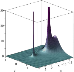
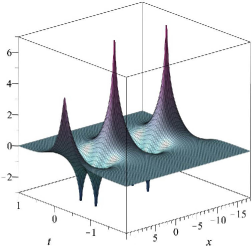
Figure 1: $|\widetilde{v}|$ (left) and $\ln|\widetilde{\rho}|$ (right).

Case 2. When $p=1$, $C_{1}=\begin{bmatrix}c_{11}\\ c_{12}\end{bmatrix}$ and $C_{2}=\begin{bmatrix}0\\ c_{22}\end{bmatrix}$ $(c_{11},\,c_{12},\,c_{22}\in{\mathbb{R}})$, our choice of non-diagonal $A$ leads to polynomials

$$\gamma_{1}:=\mathrm{i}c_{12}x-2c_{11}-4c_{12}t/\bar{a}^{2}\quad{\mathrm{and}}\quad\gamma_{2}:=\mathrm{i}c_{12}x-2c_{11}-4c_{12}t/a^{2}$$

(in addition to the exponents) in the formulas for $\widetilde{v}$ and $\widetilde{\rho}$. Namely, we have:

$$\widetilde{v}=2a_{1}c_{22}\frac{c_{22}^{2}(a_{1}\gamma_{1}-2c_{12})\mathrm{e}^{\mathrm{i}ax/2+2t/a}+c_{12}^{2}(a_{1}\gamma_{2}+2c_{12})\mathrm{e}^{-\mathrm{i}\bar{a}x/2-2t/\bar{a}}}{c_{22}^{4}\mathrm{e}^{\mathrm{i}a_{1}x+4a_{1}t/|a|^{2}}+c_{12}^{4}\mathrm{e}^{-\mathrm{i}a_{1}x-4a_{1}t/|a|^{2}}-2c_{12}^{2}c_{22}^{2}-a_{1}^{2}c_{22}^{2}\gamma_{1}\gamma_{2}},$$

$$\widetilde{\rho}=\mathrm{i}+\frac{8\mathrm{i}a_{1}^{2}c_{22}^{2}}{|a|^{4}\big{(}c_{22}^{4}\mathrm{e}^{\mathrm{i}a_{1}x+4a_{1}t/|a|^{2}}+c_{12}^{4}\mathrm{e}^{-\mathrm{i}a_{1}x-4a_{1}t/|a|^{2}}-2c_{12}^{2}c_{22}^{2}-a_{1}^{2}c_{22}^{2}\gamma_{1}\gamma_{2}\big{)}^{2}}$$

$$\qquad{}\times\Big{(}c_{22}^{4}(a_{1}\bar{a}\gamma_{1}+2\mathrm{i}a_{2}c_{12})(a_{1}a\gamma_{2}-2\mathrm{i}a_{2}c_{12})\mathrm{e}^{\mathrm{i}a_{1}x+4a_{1}t/|a|^{2}}$$

$$\qquad\quad{}+c_{12}^{4}(a_{1}\bar{a}\gamma_{1}-2\mathrm{i}a_{2}c_{12})(a_{1}a\gamma_{2}+2\mathrm{i}a_{2}c_{12})\mathrm{e}^{-\mathrm{i}a_{1}x-4a_{1}t/|a|^{2}}$$

$$\qquad\quad{}+2c_{12}^{2}c_{22}^{2}\big{(}-a_{1}^{2}(a_{1}^{2}-a_{2}^{2})\gamma_{1}\gamma_{2}+32(\mathrm{i}c_{12}x-2c_{11})c_{12}a_{2}^{2}a_{1}^{4}|a|^{-4}t-4a_{2}^{2}c_{12}^{2}\big{)}\Big{)}.$$

The behaviour of $\widetilde{v}$ and $\widetilde{\rho}$ is in this case more complicated, see Figure 2, where

$$p=1,\quad a=\frac{1}{3}+\frac{1}{5}\mathrm{i},\quad c_{11}=3,\quad c_{12}=1,\quad c_{22}=\frac{1}{2}.$$

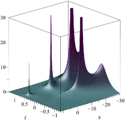
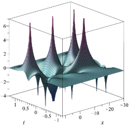
Figure 2: $|\widetilde{v}|$ (left) and $\ln|\widetilde{\rho}|$ (right).

In some other cases the formulas are more complicated and we restrict ourselves to figures only. See Figure 3, where

$$p=1,\quad a=\frac{1}{2}+\frac{1}{3}\mathrm{i},\quad C_{1}=\begin{bmatrix}1\\ 2\mathrm{i}\end{bmatrix},\quad C_{2}=\begin{bmatrix}3\mathrm{i}\\ 4\end{bmatrix};$$

see Figure 4, where

$$p=0,\quad a=\frac{3}{2}+\frac{1}{2}\mathrm{i},\quad C_{1}=\begin{bmatrix}1+3\mathrm{i}\\ 3+2\mathrm{i}\end{bmatrix},\quad C_{2}=\begin{bmatrix}6+\mathrm{i}\\ 2-4\mathrm{i}\end{bmatrix};$$

and see Figure 5, where

$$p=1,\quad a=1+\mathrm{i},\quad C_{1}=\begin{bmatrix}\mathrm{i}\\ 1\end{bmatrix},\quad C_{2}=\begin{bmatrix}1\\ \mathrm{i}\end{bmatrix}.$$

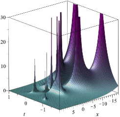
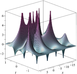
Figure 3: $|\widetilde{v}|$ (left) and $\ln|\widetilde{\rho}|$ (right).

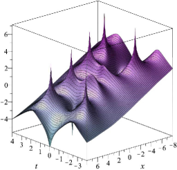
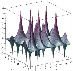
Figure 4: $\ln|\widetilde{v}|$ (left) and $\ln|\widetilde{\rho}|$ (right).

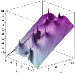
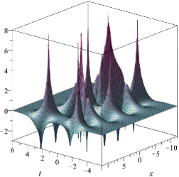
Figure 5: $\ln|\widetilde{v}|$ (left) and $\ln|\widetilde{\rho}|$ (right).

Acknowledgments. This research was supported by the Austrian Science Fund (FWF) under Grant No. P29177.

References

- [1] Ablowitz M J and Musslimani Z H 2013 Integrable nonlocal nonlinear Schrödinger equation Phys. Rev. Lett. 110 Paper 064105
- [2] Ablowitz M J and Musslimani Z H 2017 Integrable nonlocal nonlinear equations, Stud. Appl. Math. 139 7–59.
- [3] Ablowitz M J, Prinari B and Trubatch A D 2004 Discrete and continuous nonlinear Schrödinger systems (Cambridge: Cambridge University Press)
- [4] Chen K, Deng X, Lou S and Zhang D 2018 Solutions of nonlocal equations reduced from the AKNS hierarchy Stud. Appl. Math. 141 113–141.
- [5] Cieslinski J L 2009 Algebraic construction of the Darboux matrix revisited J. Phys. A 42 Paper 404003.
- [6] Deift P A 1978 Applications of a commutation formula Duke Math. J. 45 267–310.
- [7] Feng B F, Maruno K and Ohta Y 2017 Geometric formulation and multi-dark soliton solution to the defocusing complex short pulse equation Stud. Appl. Math. 138 343–367.
- [8] Fritzsche B, Kirstein B, Roitberg I and Sakhnovich A L 2017 Stability of the procedure of explicit recovery of skew-selfadjoint Dirac systems from rational Weyl matrix functions Linear Algebra Appl. 533 428–450.
- [9] Gadzhimuradov T A and Agalarov A M 2016 Towards a gauge-equivalentmagnetic structure of the nonlocal nonlinear Schrödinger equation Phys Rev A 93 Paper 062124.
- [10] Gerdjikov V S, Grahovski G G and Ivanov R I 2017 On integrable wave interactions and Lax pairs on symmetric spaces Wave Motion 71 53–70.
- [11] Gesztesy F and Teschl G 1996 On the double commutation method Proc. Amer. Math. Soc. 124 1831–1840.
- [12] Gu C, Hu H and Zhou X 2005 Darboux transformations in integrable systems (Dordrecht: Springer).
- [13] Gürses M and Pekcan A 2018 Nonlocal nonlinear Schrödinger equations and their soliton solutions J. Math. Phys. 59 Paper 051501.
- [14] Hassan M 2009 Darboux transformation of the generalized coupled dispersionless integrable system J. Phys. A 42 Paper 065203.
- [15] Kakuhata H and Konno K 1996 A generalization of coupled integrable dispersionless system J. Phys. Soc. Japan 65 340–341.
- [16] Kakuhata H and Konno K 1997 Canonical formulation of a generalized coupled dispersionless system J. Phys. A 30 L401–L407.
- [17] Konno K and Oono H 1994 New coupled integrable dispersionless equations J. Phys. Soc. Japan 63 377–378.
- [18] Kostenko A, Sakhnovich A and Teschl G 2012 Commutation methods for Schrödinger operators with strongly singular potentials Math. Nachr. 285 392–410.
- [19] Kuetche V K, Bouetou T B and Kofane T C 2008 On exact -loop soliton solution to nonlinear coupled dispersionless evolution equations Phys. Lett. A 372 665–669.
- [20] Li Z 2016 Finite-band solutions of the coupled dispersionless hierarchy J. Phys. A 49 Paper 345202.
- [21] Marchenko V A 1988 Nonlinear equations and operator algebras (Dordrecht: D. Reidel).
- [22] Matveev V B and Salle M A 1991 Darboux transformations and solitons (Berlin: Springer)
- [23] Michor J and Sakhnovich A L 2019 GBDT and algebro-geometric approaches to explicit solutions and wave functions for nonlocal NLS J. Phys. A: Math. Theor. 52 Paper 025201.
- [24] Olmedilla E 1986 Multiple pole solutions of the non-linear Schrödinger equation Physica D 25 330–346.
- [25] Sakhnovich A L 1994 Dressing procedure for solutions of nonlinear equations and the method of operator identities Inverse Problems 10 699–710.
- [26] Sakhnovich A L 2001 Generalized Bäcklund–Darboux transformation: spectral properties and nonlinear equations J. Math. Anal. Appl. 262 274–306.
- [27] Sakhnovich A L 2012 On the compatibility condition for linear systems and a factorization formula for wave functions J. Differential Equations 252 3658–3667.
- [28] Sakhnovich A L 2016 Inverse problems for self-adjoint Dirac systems: explicit solutions and stability of the procedure Oper. Matrices 10 997–1008.
- [29] Sakhnovich A L 2018 Scattering for general-type Dirac systems on the semi-axis: reflection coefficients and Weyl functions J. Differential Equations 265 4820–4834.
- [30] Sakhnovich A L, Sakhnovich L A and Roitberg I Ya 2013 Inverse problems and nonlinear evolution equations. Solutions, Darboux matrices and Weyl–Titchmarsh functions (De Gruyter Studies in Mathematics 47) (Berlin: De Gruyter).
- [31] Sakhnovich L A 1976 On the factorization of the transfer matrix function Sov. Math. Dokl. 17 203–207.
- [32] Sakhnovich L A 1999 Spectral theory of canonical differential systems, method of operator identities (Operator Theory Adv. Appl. 107) (Basel: Birkhäuser).
- [33] Schiebold C 2017 Asymptotics for the multiple pole solutions of the nonlinear Schrödinger equation Nonlinearity 30 2930–2981.
Faculty of Mathematics, University of Vienna,
Oskar-Morgenstern-Platz 1, A-1090 Vienna, Austria.
R.O. Popovych, e-mail: roman.popovych@univie.ac.at
A.L. Sakhnovich, e-mail: oleksandr.sakhnovych@univie.ac.at