Doubly-Adaptive Artificial Compression Methods for Incompressible Flow

   William Layton Department of Mathematics, University of Pittsburgh, Pittsburgh, PA 15260, USA, wjl@pitt.edu; The research herein was partially supported by NSF grants DMS1522267, 1817542 and CBET 1609120.    Michael McLaughlin Department of Mathematics, University of Pittsburgh, Pittsburgh, PA 15260, USA, mem266@pitt.edu; The research herein was partially supported by NSF grants DMS1522267, 1817542 and CBET 1609120.
Abstract

This report presents adaptive artificial compression methods in which the time-step and artificial compression parameter ε𝜀\varepsilon are independently adapted. The resulting algorithms are supported by analysis and numerical tests. The first and second-order methods are embedded. As a result, the computational, cognitive and space complexities of the adaptive ε,k𝜀𝑘\varepsilon,k algorithms are negligibly greater than that of the simplest, first-order, constant ε,𝜀\varepsilon, constant k𝑘k artificial compression method.

1 Introduction

Artificial compression (AC) methods are based on replacing u=0𝑢0\nabla\cdot u=0 by εpt+u=0𝜀subscript𝑝𝑡𝑢0\varepsilon p_{t}+\nabla\cdot u=0 (0<ε0𝜀0<\varepsilon small), uncoupling velocity and pressure and advancing the pressure explicitly in time. Their high speed and low storage requirements recommend them for complexity bound fluid flow simulations. Unfortunately, time-accurate artificial compression approximations have proven elusive. Time accuracy (along with increased efficiency and decreased memory) is obtained by time-adaptive algorithms. To our knowledge, the defect correction based scheme of Guermond and Minev [17] and the non-autonomous AC method in [6], both adapting the time-step with ε=k𝜀𝑘\varepsilon=k (time-step), are the only previous implicit, time-adaptive AC methods.

This report presents time-adaptive AC algorithms based on a new approach of independently adapting the AC parameter ε𝜀\varepsilon and time-step k𝑘k. The methods proceed as follows. A standard, first-order, implicit method, (1st Order) below, is used to advance the momentum equation in the artificial compression equations. A second-order velocity approximation, (2nd Order) below, is then computed at negligible cost using a time filter adapted from [19]. The difference between the first-order and second-order approximations gives a reliable estimator, EST(1), for the local error in the momentum equation for the first-order method and is used to adapt the time step in Algorithm 4.1, Section 4.

Adapting the AC parameter ε𝜀\varepsilon is more challenging. Stability of the standard AC discrete continuity equation (εpt+u=0𝜀subscript𝑝𝑡𝑢0\varepsilon p_{t}+\nabla\cdot u=0) is unknown for variable ε𝜀\varepsilon, [6]. We present two new, variable ε,𝜀\varepsilon, discrete continuity equations in (1.4) below and prove their unconditional, long-time stability in Theorems 2.1, 2.2 and 3.2. These results show that adaptivity will respond to accuracy constraints rather than try to correct stability problems with small time-steps. In these continuity equations, the size of unorm𝑢||\nabla\cdot u|| is monitored and used to adapt the choice of the AC parameter ε𝜀\varepsilon (e.g., Algorithm 3.1, Section 3) whereupon the calculation proceeds to the next time step. The self-adaptive strategy for independently adapting ε𝜀\varepsilon also side steps the practical problem of how to pick ε𝜀\varepsilon in AC methods and related penalty methods, even for constant time-steps. The new discrete continuity equations reduce to the standard εpt+u=0𝜀subscript𝑝𝑡𝑢0\varepsilon p_{t}+\nabla\cdot u=0 for constant ε𝜀\varepsilon, improve, through greater simplicity, a non-autonomous (ε=ε(t)𝜀𝜀𝑡\varepsilon=\varepsilon(t)) AC formulation in [6] and yield now three proven stable extensions of the discrete AC continuity equation to variable ε𝜀\varepsilon. A comparison of the three is presented in Section 5. Determining if one or some combination of the three111The stability proof extends to weighted averages of the three discrete continuity equations. or some other, yet undetermined, possibility is to be preferred is an important open problem.

The second-order method. To obtain an 𝒪(k2)𝒪superscript𝑘2\mathcal{O}(k^{2}) approximation of the momentum equation (with embedded error estimator), Algorithms 4.1 and 4.2 incorporate a recent idea of [19] of increasing accuracy and estimating errors by time filters. Theorem 3.2 of Section 3.1 gives a proof of unconditional, long-time stability of the second order, constant time-step but variable ε𝜀\varepsilon method. The resulting embedded structure of Algorithms 4.1 and 4.2 suggests low-complexity, variable-order methods may be possible once an adaptive ε𝜀\varepsilon strategy is well developed.

The second-order method is a one leg method. Reliable estimators of the local truncation error (LTE) in one leg methods are expensive as detailed in [10]. An inexpensive estimator, EST(2) in Algorithm 4.2, of the LTE in the method’s linear multistep twin, based on a second time filter, is presented. For the one leg method, this estimator is inexpensive but heuristic. The doubly adapted, second-order method in Algorithm 4.2 is tested in Section 5. The embedded structure of the first and second-order method suggests that adapting the method order in addition to the time-step and AC parameter ε𝜀\varepsilon may increase accuracy and efficiency further.

Three stable treatments of the momentum equation (first, second and even variable order) are possible. Three stable treatments of the variable ε𝜀\varepsilon continuity are now possible: two in (1.1) below and one in [6]. The result is nine adaptive AC methods with computational complexity comparable to the common first-order method, described next.

1.1 Review of a Common Artificial Compression Method

Denote by u𝑢u the velocity, p𝑝p the pressure, ν𝜈\nu the kinematic viscosity, and f𝑓f the external force. Consider the slightly compressible/hyposonic222We do not include a traditional superscript ”ε𝜀\varepsilon” as we shall focus only on AC models and methods., [38], approximation to the incompressible Navier-Stokes equations in a domain ΩΩ\Omega in d,d=2,3formulae-sequencesuperscript𝑑𝑑23{{\mathbb{R}}}^{d},d=2,3

{ut+uu+12(u)u+pνΔu=fεpt+u=0, where 0<ε is small.casessubscript𝑢𝑡𝑢𝑢12𝑢𝑢𝑝𝜈Δ𝑢𝑓otherwiseformulae-sequence𝜀subscript𝑝𝑡𝑢0 where 0𝜀 is small.otherwise\begin{cases}u_{t}+u\cdot\nabla u+{\frac{1}{2}}(\nabla\cdot u)u+\nabla p-\nu\Delta u=f\\ \varepsilon p_{t}+\nabla\cdot u=0,\text{ where }0<\varepsilon\text{ is small.}\end{cases} (1)

This is the most common of several possible formulations reviewed in Section 1.1 of [6]. To present methods herein we will consistently suppress the secondary spacial discretization333All stability results proven herein hold, by the same proof, for standard variational spatial discretizations such as finite element methods with div-stable elements.. Let usuperscript𝑢u^{\ast} denote the standard (second order) linear extrapolation of u𝑢u from previous values444Temperton and Staniforth [33] advocated even higher order extrapolation. to tn+1subscript𝑡𝑛1t_{n+1}

u=(1+kn+1kn)unkn+1knun1(=2unun1 for constant time-step).superscript𝑢annotated1subscript𝑘𝑛1subscript𝑘𝑛subscript𝑢𝑛subscript𝑘𝑛1subscript𝑘𝑛subscript𝑢𝑛1absent2subscript𝑢𝑛subscript𝑢𝑛1 for constant time-stepu^{\ast}=\left(1+\frac{k_{n+1}}{k_{n}}\right)u_{n}-\frac{k_{n+1}}{k_{n}}u_{n-1}\left(=2u_{n}-u_{n-1}\text{ for constant time-step}\right).

To fix ideas, among many possible, e.g., [14], [15], [16], [22], [24], [27], [9], [26], [37], consider a common, constant time-step, semi-implicit time discretization of (1):

un+1unk+uun+1+12(u)un+1+pn+1νΔun+1=f(tn+1),subscript𝑢𝑛1subscript𝑢𝑛𝑘superscript𝑢subscript𝑢𝑛112superscript𝑢subscript𝑢𝑛1subscript𝑝𝑛1𝜈Δsubscript𝑢𝑛1𝑓subscript𝑡𝑛1\displaystyle\frac{u_{n+1}-u_{n}}{k}+u^{\ast}\cdot\nabla u_{n+1}+{\frac{1}{2}}(\nabla\cdot u^{\ast})u_{n+1}+\nabla p_{n+1}-\nu\Delta u_{n+1}=f(t_{n+1}), (2)
 εpn+1pnk+un+1=0. 𝜀subscript𝑝𝑛1subscript𝑝𝑛𝑘subscript𝑢𝑛10\displaystyle{\text{ \ \ \ }}\varepsilon\frac{p_{n+1}-p_{n}}{k}+\nabla\cdot u_{n+1}=0.

Here k𝑘k is the time-step, tn=nk,subscript𝑡𝑛𝑛𝑘t_{n}=nk, unsubscript𝑢𝑛u_{n}, pnsubscript𝑝𝑛p_{n} are approximations to the velocity and pressure at t=tn𝑡subscript𝑡𝑛t=t_{n}. This has consistency error 𝒪(k+ε)𝒪𝑘𝜀\mathcal{O}(k+\varepsilon) leading to the most common choice of selecting ε=k𝜀𝑘\varepsilon=k to balance errors. Since pn+1=subscript𝑝𝑛1absent\nabla p_{n+1}= pn(k/ε)un+1subscript𝑝𝑛𝑘𝜀subscript𝑢𝑛1\nabla p_{n}-(k/\varepsilon)\nabla\nabla\cdot u_{n+1}, this uncouples into a velocity solve followed by an algebraic pressure update

un+1unk+uun+1+12(u)un+1kεun+1subscript𝑢𝑛1subscript𝑢𝑛𝑘superscript𝑢subscript𝑢𝑛112superscript𝑢subscript𝑢𝑛1𝑘𝜀subscript𝑢𝑛1\displaystyle\frac{u_{n+1}-u_{n}}{k}+u^{\ast}\cdot\nabla u_{n+1}+{\frac{1}{2}}(\nabla\cdot u^{\ast})u_{n+1}-\frac{k}{\varepsilon}\nabla\nabla\cdot u_{n+1}
νΔun+1=pn+fn+1,𝜈Δsubscript𝑢𝑛1subscript𝑝𝑛subscript𝑓𝑛1\displaystyle-\nu\Delta u_{n+1}=-\nabla p_{n}+f_{n+1},
 then given un+1pn+1=pnkεun+1. then given subscript𝑢𝑛1subscript𝑝𝑛1subscript𝑝𝑛𝑘𝜀subscript𝑢𝑛1\displaystyle{\text{ {then given }}u_{n+1}\text{{: \ \ \ }}}p_{n+1}=p_{n}-\frac{k}{\varepsilon}\nabla\cdot u_{n+1}. (3)

For constant ε,k𝜀𝑘\varepsilon,k, this method is unconditionally, nonlinearly, long-time stable, e.g., [14], [15], [31], [30]. Its long-time stability for variable ε,k𝜀𝑘\varepsilon,k is an open problem, [6].

1.2 New Methods for Variable ε,k𝜀𝑘\varepsilon,k

Although well motivated, the  choice ε=k𝜀𝑘\varepsilon=k cannot be more than a step to a correct choice. First observe that Units(ε)=Time2/Length3𝑈𝑛𝑖𝑡𝑠𝜀𝑇𝑖𝑚superscript𝑒2𝐿𝑒𝑛𝑔𝑡superscript3Units(\varepsilon)=Time^{2}/Length^{3} while Units(k)=Time𝑈𝑛𝑖𝑡𝑠𝑘𝑇𝑖𝑚𝑒Units(k)=Time. Thus, a correct choice of ε𝜀\varepsilon should be scaled to be dimensionally consistent and afterwards the constant multiplier optimized. Aside from dimensional inconsistency, the standard choice ε=k𝜀𝑘\varepsilon=k ignores the different roles of ε𝜀\varepsilon and k𝑘k. To leading orders, the consistency error in the continuity equation is 𝒪(ε)𝒪𝜀\mathcal{O}(\varepsilon), independent of k𝑘k, and the consistency error in the momentum equation is 𝒪(k)𝒪𝑘\mathcal{O}(k), independent of ε𝜀\varepsilon. This observation on the standard method (2), (3) motivates the development plan for the doubly adaptive algorithms herein:

  • Develop first (Section 2) and second (Section 3) order methods stable for variable k,ε𝑘𝜀k,\varepsilon.

  • Adapt εnsubscript𝜀𝑛\varepsilon_{n} to control the consistency error in the continuity equation by monitoring unorm𝑢||\nabla\cdot u||, Sections 3, 4.

  • Develop inexpensive estimators for momentum equation consistency error and adapt k=kn𝑘subscript𝑘𝑛k=k_{n} for its control, Section 4.

  • Use (Section 4) and test (Section 5) the estimators in a doubly adaptive, variable ε,k𝜀𝑘\varepsilon,k, algorithm.

In adaptive methods, strong stability is necessary, so εn,knsubscript𝜀𝑛subscript𝑘𝑛\varepsilon_{n},k_{n} can be adapted for time-accuracy rather than to correct instabilities. One key difficulty, resolved by the two methods (4) below, is that useful stability is unknown for the common AC method (2) with variable ε𝜀\varepsilon, see [6], and even for the continuum model (1) with ε=ε(t)𝜀𝜀𝑡\varepsilon=\varepsilon(t). A second key difficulty is that (unconditional, nonlinear) G-stability for variable time-steps is uncommon555To our knowledge, the only such two-step method is the little explored one of Dahlquist, Liniger, and Nevanlinna [7]. This second issue may be resolvable by a variable (first and second) order implementation since it would include the A-stable, fully implicit method.. (For example, the popular BDF2 method loses Alimit-from𝐴A-stability for increasing time-steps.)

The continuity equation is treated by either a geometric average (GA-Method) or a minimum term (min-Method) as follows. Given un,pn,εnsubscript𝑢𝑛subscript𝑝𝑛subscript𝜀𝑛u_{n},p_{n},\varepsilon_{n}, select εn+1,kn+1subscript𝜀𝑛1subscript𝑘𝑛1\varepsilon_{n+1},k_{n+1} calculate un+1subscript𝑢𝑛1u_{n+1} then666A convex combination of the two continuity equations discretizations is also stable.

GA-Method:εn+1pn+1εn+1εnpnkn+1+un+1=0, ormin-Method:εn+1pn+1min{εn+1,εn}pnkn+1+un+1=0.GA-Method:missing-subexpressionsubscript𝜀𝑛1subscript𝑝𝑛1subscript𝜀𝑛1subscript𝜀𝑛subscript𝑝𝑛subscript𝑘𝑛1subscript𝑢𝑛10 ormissing-subexpressionmissing-subexpressionmissing-subexpressionmin-Method:missing-subexpressionsubscript𝜀𝑛1subscript𝑝𝑛1subscript𝜀𝑛1subscript𝜀𝑛subscript𝑝𝑛subscript𝑘𝑛1subscript𝑢𝑛10\begin{array}[]{ccc}\text{GA-Method:}&&\frac{\varepsilon_{n+1}p_{n+1}-\sqrt{\varepsilon_{n+1}\varepsilon_{n}}p_{n}}{k_{n+1}}+\nabla\cdot u_{n+1}=0,\text{ or}\\ &&\\ \text{min-Method:}&&\frac{\varepsilon_{n+1}p_{n+1}-\min\{\varepsilon_{n+1},\varepsilon_{n}\}p_{n}}{k_{n+1}}+\nabla\cdot u_{n+1}=0.\end{array} (4)

These methods are proven in Section 2 to be unconditionally, variable ε,k𝜀𝑘\varepsilon,k stable. For the discrete momentum equation, recall usuperscript𝑢u^{\ast} is an extrapolated approximation to u(tn+1)𝑢subscript𝑡𝑛1u(t_{n+1}). The first-order method’s momentum equation is the standard one (2) above given by

un+1unkn+1+uun+1+12(u)un+1+pn+1νΔun+1=fn+1.subscript𝑢𝑛1subscript𝑢𝑛subscript𝑘𝑛1superscript𝑢subscript𝑢𝑛112superscript𝑢subscript𝑢𝑛1subscript𝑝𝑛1𝜈Δsubscript𝑢𝑛1subscript𝑓𝑛1\frac{u_{n+1}-u_{n}}{k_{n+1}}+u^{\ast}\cdot\nabla u_{n+1}+{\frac{1}{2}}(\nabla\cdot u^{\ast})u_{n+1}+\nabla p_{n+1}-\nu\Delta u_{n+1}=f_{n+1}. (1st Order)

The (linearly implicit) treatment of the nonlinear term is inspired by Baker [4]. The second method, adapted from [19], adds a time filter to obtain 𝒪(k2)𝒪superscript𝑘2\mathcal{O}(k^{2}) accuracy and automatic error estimation as follows. Let the time-step ratio be denoted τ=kn+1/kn𝜏subscript𝑘𝑛1subscript𝑘𝑛\tau=k_{n+1}/k_{n}. Call un+11superscriptsubscript𝑢𝑛11u_{n+1}^{1} the solution obtained from the first-order method (1st Order) above. The second-order approximation un+1subscript𝑢𝑛1u_{n+1} is obtained by filtering un+11superscriptsubscript𝑢𝑛11u_{n+1}^{1}:

un+11unkn+1+uun+11+12(u)un+11+pn+1νΔun+11=fn+1,For τ=kn+1kn let α1=τ(1+τ)(1+2τ), then:un+1=un+11α12{2knkn+kn+1un+112un+2kn+1kn+kn+1un1}.\begin{split}\frac{u_{n+1}^{1}-u_{n}}{k_{n+1}}&+u^{\ast}\cdot\nabla u_{n+1}^{1}+{\frac{1}{2}}(\nabla\cdot u^{\ast})u_{n+1}^{1}+\nabla p_{n+1}-\nu\Delta u_{n+1}^{1}=f_{n+1},\\ \text{For }\tau&=\frac{k_{n+1}}{k_{n}}\text{ let }\alpha_{1}=\frac{\tau(1+\tau)}{(1+2\tau)},\text{ then}:\\ u_{n+1}&=u_{n+1}^{1}-\frac{\alpha_{1}}{2}\left\{\frac{2k_{n}}{k_{n}+k_{n+1}}u_{n+1}^{1}-2u_{n}+\frac{2k_{n+1}}{k_{n}+k_{n+1}}u_{n-1}\right\}.\end{split} (2nd Order)

Denote by D2(n+1)subscript𝐷2𝑛1D_{2}(n+1) the quantity above in braces

D2(n+1):=2knkn+kn+1un+112un+2kn+1kn+kn+1un1.assignsubscript𝐷2𝑛12subscript𝑘𝑛subscript𝑘𝑛subscript𝑘𝑛1superscriptsubscript𝑢𝑛112subscript𝑢𝑛2subscript𝑘𝑛1subscript𝑘𝑛subscript𝑘𝑛1subscript𝑢𝑛1D_{2}(n+1):=\frac{2k_{n}}{k_{n}+k_{n+1}}u_{n+1}^{1}-2u_{n}+\frac{2k_{n+1}}{k_{n}+k_{n+1}}u_{n-1}.

Note that D2(n+1)subscript𝐷2𝑛1D_{2}(n+1) is 2knkn+1×2k_{n}k_{n+1}\times(a second divided difference).

The usual L2superscript𝐿2L^{2} norm ||||||\cdot|| and inner product (,)(\cdot,\cdot) are denoted

v=(Ω|v(x)|2𝑑x)1/2 and (v,w)=Ωv(x)w(x)𝑑x.norm𝑣superscriptsubscriptΩsuperscript𝑣𝑥2differential-d𝑥12 and 𝑣𝑤subscriptΩ𝑣𝑥𝑤𝑥differential-d𝑥||v||=\left(\int_{\Omega}|v(x)|^{2}dx\right)^{1/2}\text{ and }(v,w)=\int_{\Omega}v(x)\cdot w(x)dx.

A simple estimate of the local error in the first-order approximation un+11superscriptsubscript𝑢𝑛11u_{n+1}^{1} is given by a measure (here the L2superscript𝐿2L^{2} norm) of the difference of the two approximations

EST(1)=un+1un+11=α12D2(n+1).𝐸𝑆𝑇1normsubscript𝑢𝑛1superscriptsubscript𝑢𝑛11subscript𝛼12normsubscript𝐷2𝑛1EST(1)=||u_{n+1}-u_{n+1}^{1}||=\frac{\alpha_{1}}{2}||D_{2}(n+1)||.

Estimating the error in the second-order approximation. Naturally one would like to use the second-order approximation for more than an estimator. It is possible to use EST(1)𝐸𝑆𝑇1EST(1) above as a pessimistic estimator for un+1subscript𝑢𝑛1u_{n+1}. In Section 3 we show that, eliminating the intermediate step un+11superscriptsubscript𝑢𝑛11u_{n+1}^{1}, the second-order method is equivalent to the second-order, one leg method (13) below. Estimation of the LTE for this OLM cannot be done by a simple time filter for reasons delineated in [10] and based on classical analysis of the LTE in OLMs of Dahlquist. We test an inexpensive but heuristic estimator that can be calculated by a second time filter. EST(2)𝐸𝑆𝑇2EST(2) below is an LTE estimator for the OLMs linear multi-step twin. To estimate the local error in the second order approximation we use the third divided difference with multiplier chosen (by a lengthy but elementary Taylor series calculation) to cancel the first term of the LTE of the methods linear multi-step twin

EST(2)𝐸𝑆𝑇2\displaystyle EST(2) =\displaystyle= α263kn1kn+1+kn+kn1D2(n+1)3kn1kn+1+kn+kn1D2(n)subscript𝛼26norm3subscript𝑘𝑛1subscript𝑘𝑛1subscript𝑘𝑛subscript𝑘𝑛1subscript𝐷2𝑛13subscript𝑘𝑛1subscript𝑘𝑛1subscript𝑘𝑛subscript𝑘𝑛1subscript𝐷2𝑛\displaystyle\frac{\alpha_{2}}{6}\left\|\frac{3k_{n-1}}{k_{n+1}+k_{n}+k_{n-1}}D_{2}(n+1)-\frac{3k_{n-1}}{k_{n+1}+k_{n}+k_{n-1}}D_{2}(n)\right\|
where
α2subscript𝛼2\displaystyle\alpha_{2} =\displaystyle= τn(τn+1τn+τn+1)(4τn+13+5τn+12+τn+1)3(τnτn+12+4τnτn+1+2τn+1+τn+1), and τn=kn/kn1.subscript𝜏𝑛subscript𝜏𝑛1subscript𝜏𝑛subscript𝜏𝑛14superscriptsubscript𝜏𝑛135superscriptsubscript𝜏𝑛12subscript𝜏𝑛13subscript𝜏𝑛superscriptsubscript𝜏𝑛124subscript𝜏𝑛subscript𝜏𝑛12subscript𝜏𝑛1subscript𝜏𝑛1 and subscript𝜏𝑛subscript𝑘𝑛subscript𝑘𝑛1\displaystyle\frac{\tau_{n}(\tau_{n+1}\tau_{n}+\tau_{n}+1)(4\tau_{n+1}^{3}+5\tau_{n+1}^{2}+\tau_{n+1})}{3(\tau_{n}\tau_{n+1}^{2}+4\tau_{n}\tau_{n+1}+2\tau_{n+1}+\tau_{n}+1)},\text{ and }\tau_{n}=k_{n}/k_{n-1}.

The resulting adaptive algorithm uncouples like (3) into a velocity update with a grad-div term then an algebraic pressure update. More reliable but more expensive estimators are possible. The above inexpensive but heuristic one is tested herein because the motivation for AC methods is often based on the need for faster and reduced memory algorithms in specific applications.

Section 2 presents the analysis of the two first-order methods, proving long-time, unconditional stability for variable ε,k𝜀𝑘\varepsilon,k. This analysis develops the key treatment of the discrete continuity equation necessary for stability. Section 3.1 gives a proof of unconditional, long time stability for the variable ε𝜀\varepsilon, constant k𝑘k second order method. This proof can be extended to decreasing time-steps but not increasing time-steps.

1.3 Related work

Artificial compression (AC) methods were introduced in the 1960’s by Chorin, Oskolkov and Temam. Their mathematical foundation has been extensively developed by Shen [29], [30], [31], [32] and Prohl [27]. Recent work includes [24], [9], [15], [16], [22], [26] and [37]. The GA-method (geometric averaging method) herein is motivated by work in [5] for uncoupling atmosphere-ocean problems stably.

There has been extensive development of adaptive methods for assured accuracy in fully coupled, vp𝑣𝑝v-p discretizations, e.g., [21], and adaptive methods based on estimates of local truncation errors including [20], [23], [34]. In complement, the work herein aims at methods that use less expensive local (rather than global) error estimators, do not provide assured time-accuracy but emphasize (consistent with the artificial compression methods) low cognitive, computational, and space complexity. Aside from [6] and Guermond and Minev [17], extension of implicit, time-adaptive methods to artificial compression discretizations is undeveloped.

Herein accuracy is increased and local errors estimated by time filters. Other approaches are clearly possible. Time filters are an important tool in GFD to correct weak instabilities and extend forecast horizons, [3], [25], [28], [35], [36]. In [19], it was noticed that a time filter can also increase the convergence rate of the backward Euler method and estimate errors. G-stability of the resulting (constant time-step) time discretization was recently proven for the fully-coupled, velocity-pressure Navier-Stokes equations in [11].

2 First-Order, Variable k,ε𝑘𝜀k,\varepsilon Methods

This section establishes unconditional, long-time, nonlinear stability of the two variable k,ε𝑘𝜀k,\varepsilon first-order methods of Section 1.2 in the usual L2(Ω)superscript𝐿2ΩL^{2}(\Omega) norm, denoted ||||||\cdot|| with associated inner product (,)(\cdot,\cdot). The methods differ in the treatment of the discrete continuity equation and reduce to the standard AC method (2) for constant ε,k𝜀𝑘\varepsilon,k. We prove that the first order implicit discretization of the momentum equation with both new methods (5), (6) are unconditionally, nonlinearly, long-time stable without assumptions on εn,knsubscript𝜀𝑛subscript𝑘𝑛\varepsilon_{n},k_{n}. We study these new methods in a bounded, regular domain ΩΩ\Omega subject to the initial and boundary conditions

u0=u0(x) and p0=p0(x), in Ω,formulae-sequencesubscript𝑢0subscript𝑢0𝑥 and subscript𝑝0subscript𝑝0𝑥 in Ω,\displaystyle u_{0}=u_{0}(x)\text{ and }p_{0}=p_{0}(x),\text{ in }\Omega\text{,}
un=0 on Ω for t>0.subscript𝑢𝑛0 on Ω for 𝑡0.\displaystyle u_{n}=0\text{ on }\partial\Omega\text{ \ for }t>0\text{.}

The two, first-order methods are: Given un,pn,εnsubscript𝑢𝑛subscript𝑝𝑛subscript𝜀𝑛u_{n},p_{n},\varepsilon_{n}, select εn+1,kn+1subscript𝜀𝑛1subscript𝑘𝑛1\varepsilon_{n+1},k_{n+1} and

un+1unkn+1+uun+1+12(u)un+1+pn+1νΔun+1=fn+1,subscript𝑢𝑛1subscript𝑢𝑛subscript𝑘𝑛1superscript𝑢subscript𝑢𝑛112superscript𝑢subscript𝑢𝑛1subscript𝑝𝑛1𝜈Δsubscript𝑢𝑛1subscript𝑓𝑛1\displaystyle\frac{u_{n+1}-u_{n}}{k_{n+1}}+u^{\ast}\cdot\nabla u_{n+1}+{\frac{1}{2}}(\nabla\cdot u^{\ast})u_{n+1}+\nabla p_{n+1}-\nu\Delta u_{n+1}=f_{n+1},
εn+1pn+1ε^pnkn+1+un+1=0, wheresubscript𝜀𝑛1subscript𝑝𝑛1^𝜀subscript𝑝𝑛subscript𝑘𝑛1subscript𝑢𝑛10 where\displaystyle\frac{\varepsilon_{n+1}p_{n+1}-\hat{\varepsilon}p_{n}}{k_{n+1}}+\nabla\cdot u_{n+1}=0,\text{ where}
ε^=min{εn+1,εn} for the min-Method and^𝜀subscript𝜀𝑛1subscript𝜀𝑛 for the min-Method and\displaystyle\hat{\varepsilon}=\min\{\varepsilon_{n+1},\varepsilon_{n}\}\text{ \ \ for the min-Method and} (5)
ε^=εn+1,εn for the GA-Method ^𝜀subscript𝜀𝑛1subscript𝜀𝑛 for the GA-Method \displaystyle\hat{\varepsilon}=\sqrt{\varepsilon_{n+1},\varepsilon_{n}}\text{ \ \ \ \ for the GA-Method } (6)

For constant ε𝜀\varepsilon both methods reduce to the standard method (2), (3) for which stability is known. Thus, the interest is stability for variable ε𝜀\varepsilon.

Stability of the min-Method. It is useful to recall that

(εn+1εn)+=max{0,εn+1εn}=εn+1min{0,εn+1εn}.superscriptsubscript𝜀𝑛1subscript𝜀𝑛0subscript𝜀𝑛1subscript𝜀𝑛subscript𝜀𝑛10subscript𝜀𝑛1subscript𝜀𝑛\left(\varepsilon_{n+1}-\varepsilon_{n}\right)^{+}=\max\{0,\varepsilon_{n+1}-\varepsilon_{n}\}=\varepsilon_{n+1}-\min\{0,\varepsilon_{n+1}-\varepsilon_{n}\}.
Theorem 1 (Stability of the min Method).

The variable ε,k𝜀𝑘\varepsilon,k min-Method is unconditionally, long-time stable. For any N>0𝑁0N>0 the energy equality holds:

12Ω|uN|2+εN|pN|2dx+12subscriptΩsuperscriptsubscript𝑢𝑁2limit-fromsubscript𝜀𝑁superscriptsubscript𝑝𝑁2𝑑𝑥\displaystyle\frac{1}{2}\int_{\Omega}|u_{N}|^{2}+\varepsilon_{N}|p_{N}|^{2}dx+
n=0N112Ωmin{εn+1,εn}(pn+1pn)2+(εn+1εn)+pn+12\displaystyle\sum_{n=0}^{N-1}\frac{1}{2}\int_{\Omega}\min\{\varepsilon_{n+1},\varepsilon_{n}\}(p_{n+1}-p_{n})^{2}+\left(\varepsilon_{n+1}-\varepsilon_{n}\right)^{+}p_{n+1}{}^{2}
+(εnεn+1)+pnd2x+n=0N1Ω12|un+1un|2+kn+1ν|un+1|2dxsuperscriptsubscript𝜀𝑛subscript𝜀𝑛1subscript𝑝𝑛superscript𝑑2𝑥superscriptsubscript𝑛0𝑁1subscriptΩ12superscriptsubscript𝑢𝑛1subscript𝑢𝑛2subscript𝑘𝑛1𝜈superscriptsubscript𝑢𝑛12𝑑𝑥\displaystyle+\left(\varepsilon_{n}-\varepsilon_{n+1}\right)^{+}p_{n}{}^{2}dx+\sum_{n=0}^{N-1}\int_{\Omega}\frac{1}{2}|u_{n+1}-u_{n}|^{2}+k_{n+1}\nu|\nabla u_{n+1}|^{2}dx
=12Ω|u0|2+ε0p0d2x+n=0N1kn+1Ωun+1fn+1𝑑x.absent12subscriptΩsuperscriptsubscript𝑢02subscript𝜀0subscript𝑝0superscript𝑑2𝑥superscriptsubscript𝑛0𝑁1subscript𝑘𝑛1subscriptΩsubscript𝑢𝑛1subscript𝑓𝑛1differential-d𝑥\displaystyle=\frac{1}{2}\int_{\Omega}|u_{0}|^{2}+\varepsilon_{0}p_{0}{}^{2}dx+\sum_{n=0}^{N-1}k_{n+1}\int_{\Omega}u_{n+1}\cdot f_{n+1}dx.

Consequently, the stability bound holds:

12Ω|uN|2+εNpNd2x+12subscriptΩsuperscriptsubscript𝑢𝑁2limit-fromsubscript𝜀𝑁subscript𝑝𝑁superscript𝑑2𝑥\displaystyle\frac{1}{2}\int_{\Omega}|u_{N}|^{2}+\varepsilon_{N}p_{N}{}^{2}dx+
n=0N112Ωmin{εn+1,εn}(pn+1pn)2𝑑x+(εn+1εn)+pn+12superscriptsubscript𝑛0𝑁112subscriptΩsubscript𝜀𝑛1subscript𝜀𝑛superscriptsubscript𝑝𝑛1subscript𝑝𝑛2differential-d𝑥superscriptsubscript𝜀𝑛1subscript𝜀𝑛superscriptsubscript𝑝𝑛12\displaystyle\sum_{n=0}^{N-1}\frac{1}{2}\int_{\Omega}\min\{\varepsilon_{n+1},\varepsilon_{n}\}(p_{n+1}-p_{n})^{2}dx+\left(\varepsilon_{n+1}-\varepsilon_{n}\right)^{+}p_{n+1}^{2}
+(εnεn+1)+pnd2x+n=0N112Ω|un+1un|2+kn+1ν|un+1|2dxsuperscriptsubscript𝜀𝑛subscript𝜀𝑛1subscript𝑝𝑛superscript𝑑2𝑥superscriptsubscript𝑛0𝑁112subscriptΩsuperscriptsubscript𝑢𝑛1subscript𝑢𝑛2subscript𝑘𝑛1𝜈superscriptsubscript𝑢𝑛12𝑑𝑥\displaystyle+\left(\varepsilon_{n}-\varepsilon_{n+1}\right)^{+}p_{n}{}^{2}dx+\sum_{n=0}^{N-1}\frac{1}{2}\int_{\Omega}|u_{n+1}-u_{n}|^{2}+k_{n+1}\nu|\nabla u_{n+1}|^{2}dx
12Ω|u0|2+ε0p0d2x+n=0N1kn+112νfn+112.absent12subscriptΩsuperscriptsubscript𝑢02subscript𝜀0subscript𝑝0superscript𝑑2𝑥superscriptsubscript𝑛0𝑁1subscript𝑘𝑛112𝜈superscriptsubscriptnormsubscript𝑓𝑛112\displaystyle\leq\frac{1}{2}\int_{\Omega}|u_{0}|^{2}+\varepsilon_{0}p_{0}{}^{2}dx+\sum_{n=0}^{N-1}k_{n+1}\frac{1}{2\nu}||f_{n+1}||_{-1}^{2}.
Proof.

First we note that using the polarization identity, algebraic rearrangement and considering the cases εn+1>εnsubscript𝜀𝑛1subscript𝜀𝑛\varepsilon_{n+1}>\varepsilon_{n} and εn+1<εnsubscript𝜀𝑛1subscript𝜀𝑛\varepsilon_{n+1}<\varepsilon_{n} we have

(εn+1pn+1min{εn+1,εn}pn,pn+1)subscript𝜀𝑛1subscript𝑝𝑛1subscript𝜀𝑛1subscript𝜀𝑛subscript𝑝𝑛subscript𝑝𝑛1\displaystyle(\varepsilon_{n+1}p_{n+1}-\min\{\varepsilon_{n+1},\varepsilon_{n}\}p_{n},p_{n+1})
=εn+1pn+12min{εn+1,εn}(pn,pn+1)absentsubscript𝜀𝑛1superscriptnormsubscript𝑝𝑛12subscript𝜀𝑛1subscript𝜀𝑛subscript𝑝𝑛subscript𝑝𝑛1\displaystyle=\varepsilon_{n+1}||p_{n+1}||^{2}-\min\{\varepsilon_{n+1},\varepsilon_{n}\}(p_{n},p_{n+1})
=εn+1pn+12min{εn+1,εn}{12pn2+12pn+1212pnpn+12}absentsubscript𝜀𝑛1superscriptnormsubscript𝑝𝑛12subscript𝜀𝑛1subscript𝜀𝑛12superscriptnormsubscript𝑝𝑛212superscriptnormsubscript𝑝𝑛1212superscriptnormsubscript𝑝𝑛subscript𝑝𝑛12\displaystyle=\varepsilon_{n+1}||p_{n+1}||^{2}-\min\{\varepsilon_{n+1},\varepsilon_{n}\}\left\{\frac{1}{2}||p_{n}||^{2}+\frac{1}{2}||p_{n+1}||^{2}-\frac{1}{2}||p_{n}-p_{n+1}||^{2}\right\}
=(εn+112min{εn+1,εn})pn+12absentsubscript𝜀𝑛112subscript𝜀𝑛1subscript𝜀𝑛superscriptnormsubscript𝑝𝑛12\displaystyle=\left(\varepsilon_{n+1}-\frac{1}{2}\min\{\varepsilon_{n+1},\varepsilon_{n}\}\right)||p_{n+1}||^{2}
12min{εn+1,εn}pn2+12min{εn+1,εn}pnpn+1212subscript𝜀𝑛1subscript𝜀𝑛superscriptnormsubscript𝑝𝑛212subscript𝜀𝑛1subscript𝜀𝑛superscriptnormsubscript𝑝𝑛subscript𝑝𝑛12\displaystyle-\frac{1}{2}\min\{\varepsilon_{n+1},\varepsilon_{n}\}||p_{n}||^{2}+\frac{1}{2}\min\{\varepsilon_{n+1},\varepsilon_{n}\}||p_{n}-p_{n+1}||^{2}
=12εn+1pn+1212εnpn2+12min{εn+1,εn}pnpn+12+absent12subscript𝜀𝑛1superscriptnormsubscript𝑝𝑛1212subscript𝜀𝑛superscriptnormsubscript𝑝𝑛2limit-from12subscript𝜀𝑛1subscript𝜀𝑛superscriptnormsubscript𝑝𝑛subscript𝑝𝑛12\displaystyle=\frac{1}{2}\varepsilon_{n+1}||p_{n+1}||^{2}-\frac{1}{2}\varepsilon_{n}||p_{n}||^{2}+\frac{1}{2}\min\{\varepsilon_{n+1},\varepsilon_{n}\}||p_{n}-p_{n+1}||^{2}+
+12(εn+1min{εn+1,εn})pn+12+12(εnmin{εn+1,εn})pn2.12subscript𝜀𝑛1subscript𝜀𝑛1subscript𝜀𝑛superscriptnormsubscript𝑝𝑛1212subscript𝜀𝑛subscript𝜀𝑛1subscript𝜀𝑛superscriptnormsubscript𝑝𝑛2\displaystyle+\frac{1}{2}\left(\varepsilon_{n+1}-\min\{\varepsilon_{n+1},\varepsilon_{n}\}\right)||p_{n+1}||^{2}+\frac{1}{2}\left(\varepsilon_{n}-\min\{\varepsilon_{n+1},\varepsilon_{n}\}\right)||p_{n}||^{2}.

We have εn+1min{εn+1,εn}=(εn+1εn)+subscript𝜀𝑛1subscript𝜀𝑛1subscript𝜀𝑛superscriptsubscript𝜀𝑛1subscript𝜀𝑛\varepsilon_{n+1}-\min\{\varepsilon_{n+1},\varepsilon_{n}\}=\left(\varepsilon_{n+1}-\varepsilon_{n}\right)^{+} and εnmin{εn+1,εn}=subscript𝜀𝑛subscript𝜀𝑛1subscript𝜀𝑛absent\varepsilon_{n}-\min\{\varepsilon_{n+1},\varepsilon_{n}\}=
(εnεn+1)+.superscriptsubscript𝜀𝑛subscript𝜀𝑛1\left(\varepsilon_{n}-\varepsilon_{n+1}\right)^{+}. Thus,

(εn+1pn+1min{εn+1,εn}pn,pn+1)=subscript𝜀𝑛1subscript𝑝𝑛1subscript𝜀𝑛1subscript𝜀𝑛subscript𝑝𝑛subscript𝑝𝑛1absent\displaystyle(\varepsilon_{n+1}p_{n+1}-\min\{\varepsilon_{n+1},\varepsilon_{n}\}p_{n},p_{n+1})= (7)
=12εn+1pn+1212εnpn2+12min{εn+1,εn}pnpn+12+absent12subscript𝜀𝑛1superscriptnormsubscript𝑝𝑛1212subscript𝜀𝑛superscriptnormsubscript𝑝𝑛2limit-from12subscript𝜀𝑛1subscript𝜀𝑛superscriptnormsubscript𝑝𝑛subscript𝑝𝑛12\displaystyle=\frac{1}{2}\varepsilon_{n+1}||p_{n+1}||^{2}-\frac{1}{2}\varepsilon_{n}||p_{n}||^{2}+\frac{1}{2}\min\{\varepsilon_{n+1},\varepsilon_{n}\}||p_{n}-p_{n+1}||^{2}+
+12(εn+1εn)+pn+12+12(εnεn+1)+pn2.12superscriptsubscript𝜀𝑛1subscript𝜀𝑛superscriptnormsubscript𝑝𝑛1212superscriptsubscript𝜀𝑛subscript𝜀𝑛1superscriptnormsubscript𝑝𝑛2\displaystyle+\frac{1}{2}\left(\varepsilon_{n+1}-\varepsilon_{n}\right)^{+}||p_{n+1}||^{2}+\frac{1}{2}\left(\varepsilon_{n}-\varepsilon_{n+1}\right)^{+}||p_{n}||^{2}.

With this identity, take the inner product of the first equation with kn+1un+1subscript𝑘𝑛1subscript𝑢𝑛1k_{n+1}u_{n+1}, the second with kn+1pn+1subscript𝑘𝑛1subscript𝑝𝑛1k_{n+1}p_{n+1}, integrate over the flow domain, integrate by parts, use skew symmetry, use the polarization identity twice and add. This yields

12Ω|un+1|2|un|2+|un+1un|2dx+Ωkn+1ν|un+1|2𝑑x12subscriptΩsuperscriptsubscript𝑢𝑛12superscriptsubscript𝑢𝑛2superscriptsubscript𝑢𝑛1subscript𝑢𝑛2𝑑𝑥subscriptΩsubscript𝑘𝑛1𝜈superscriptsubscript𝑢𝑛12differential-d𝑥\displaystyle\frac{1}{2}\int_{\Omega}|u_{n+1}|^{2}-|u_{n}|^{2}+|u_{n+1}-u_{n}|^{2}dx+\int_{\Omega}k_{n+1}\nu|\nabla u_{n+1}|^{2}dx
12Ω(εn+1pn+1min{εn+1,εn}pn)pn+1𝑑x=kn+1Ωun+1fn+1𝑑x.12subscriptΩsubscript𝜀𝑛1subscript𝑝𝑛1subscript𝜀𝑛1subscript𝜀𝑛subscript𝑝𝑛subscript𝑝𝑛1differential-d𝑥subscript𝑘𝑛1subscriptΩsubscript𝑢𝑛1subscript𝑓𝑛1differential-d𝑥\displaystyle\frac{1}{2}\int_{\Omega}(\varepsilon_{n+1}p_{n+1}-\min\{\varepsilon_{n+1},\varepsilon_{n}\}p_{n})p_{n+1}dx=k_{n+1}\int_{\Omega}u_{n+1}\cdot f_{n+1}dx.

From (7) the energy equality becomes

12Ω|un+1|2+εn+1|pn+1|2dx12Ω|un|2+εnpnd2x12subscriptΩsuperscriptsubscript𝑢𝑛12subscript𝜀𝑛1superscriptsubscript𝑝𝑛12𝑑𝑥12subscriptΩsuperscriptsubscript𝑢𝑛2subscript𝜀𝑛subscript𝑝𝑛superscript𝑑2𝑥\displaystyle\frac{1}{2}\int_{\Omega}|u_{n+1}|^{2}+\varepsilon_{n+1}|p_{n+1}|^{2}dx-\frac{1}{2}\int_{\Omega}|u_{n}|^{2}+\varepsilon_{n}p_{n}{}^{2}dx
+Ωkn+1ν|un+1|2𝑑x+12Ω(un+1un)2+min{εn+1,εn}(pnpn+1)2subscriptΩsubscript𝑘𝑛1𝜈superscriptsubscript𝑢𝑛12differential-d𝑥12subscriptΩsuperscriptsubscript𝑢𝑛1subscript𝑢𝑛2subscript𝜀𝑛1subscript𝜀𝑛superscriptsubscript𝑝𝑛subscript𝑝𝑛12\displaystyle+\int_{\Omega}k_{n+1}\nu|\nabla u_{n+1}|^{2}dx+\frac{1}{2}\int_{\Omega}(u_{n+1}-u_{n})^{2}+\min\{\varepsilon_{n+1},\varepsilon_{n}\}(p_{n}-p_{n+1})^{2}
+(εn+1εn)+pn+1+2(εnεn+1)+pnd2x=kn+1Ωun+1fn+1dx.\displaystyle+\left(\varepsilon_{n+1}-\varepsilon_{n}\right)^{+}p_{n+1}{}^{2}+\left(\varepsilon_{n}-\varepsilon_{n+1}\right)^{+}p_{n}{}^{2}dx=k_{n+1}\int_{\Omega}u_{n+1}\cdot f_{n+1}dx.

Upon summation the first two terms telescope, completing the proof of the energy equality. The stability estimate follows from the energy equality and the Cauchy-Schwarz-Young inequality.    


The stability analysis shows that the numerical dissipation in the min-Method is

NumericalDissipationNumericalDissipation\displaystyle\begin{array}[]{c}\text{Numerical}\\ \text{Dissipation}\end{array}\text{ } = 12kn+12Ω|un+1unkn+1|2+min{εn+1,εn}(pn+1pnkn+1)2+12superscriptsubscript𝑘𝑛12subscriptΩsuperscriptsubscript𝑢𝑛1subscript𝑢𝑛subscript𝑘𝑛12limit-fromsubscript𝜀𝑛1subscript𝜀𝑛superscriptsubscript𝑝𝑛1subscript𝑝𝑛subscript𝑘𝑛12\displaystyle\frac{1}{2}k_{n+1}^{2}\int_{\Omega}|\frac{u_{n+1}-u_{n}}{k_{n+1}}|^{2}+\min\{\varepsilon_{n+1},\varepsilon_{n}\}(\frac{p_{n+1}-p_{n}}{k_{n+1}})^{2}+
+(εn+1εnkn+1)+pn+12+(εnεn+1kn+1)+pnd2x.superscriptsubscript𝜀𝑛1subscript𝜀𝑛subscript𝑘𝑛1superscriptsubscript𝑝𝑛12superscriptsubscript𝜀𝑛subscript𝜀𝑛1subscript𝑘𝑛1subscript𝑝𝑛superscript𝑑2𝑥\displaystyle+\left(\frac{\varepsilon_{n+1}-\varepsilon_{n}}{k_{n+1}}\right)^{+}p_{n+1}^{2}+\left(\frac{\varepsilon_{n}-\varepsilon_{n+1}}{k_{n+1}}\right)^{+}p_{n}{}^{2}dx.

The GA-Method. The proof of stability of the GA-method differs from the last proof only in the treatment of the variable ε𝜀\varepsilon term, resulting is a different numerical dissipation for the method.

Theorem 2 (Stability of GA-Method).

The variable ε,k𝜀𝑘\varepsilon,k, first-order GA-Method is unconditionally, long-time stable. For any N>0𝑁0N>0 the energy equality holds:

12Ω|uN|2+εN|pN|2dx+12subscriptΩsuperscriptsubscript𝑢𝑁2limit-fromsubscript𝜀𝑁superscriptsubscript𝑝𝑁2𝑑𝑥\displaystyle\frac{1}{2}\int_{\Omega}|u_{N}|^{2}+\varepsilon_{N}|p_{N}|^{2}dx+
+n=0N112Ω|un+1un|2+(εn+1pn+1εnpn)2+2kn+1ν|un+1|2dxsuperscriptsubscript𝑛0𝑁112subscriptΩsuperscriptsubscript𝑢𝑛1subscript𝑢𝑛2superscriptsubscript𝜀𝑛1subscript𝑝𝑛1subscript𝜀𝑛subscript𝑝𝑛22subscript𝑘𝑛1𝜈superscriptsubscript𝑢𝑛12𝑑𝑥\displaystyle+\sum_{n=0}^{N-1}\frac{1}{2}\int_{\Omega}|u_{n+1}-u_{n}|^{2}+(\sqrt{\varepsilon_{n+1}}p_{n+1}-\sqrt{\varepsilon_{n}}p_{n})^{2}+2k_{n+1}\nu|\nabla u_{n+1}|^{2}dx
=12Ω|u0|2+ε0|p0|2dx+n=0N1kn+1Ωun+1fn+1𝑑xabsent12subscriptΩsuperscriptsubscript𝑢02subscript𝜀0superscriptsubscript𝑝02𝑑𝑥superscriptsubscript𝑛0𝑁1subscript𝑘𝑛1subscriptΩsubscript𝑢𝑛1subscript𝑓𝑛1differential-d𝑥\displaystyle=\frac{1}{2}\int_{\Omega}|u_{0}|^{2}+\varepsilon_{0}|p_{0}|^{2}dx+\sum_{n=0}^{N-1}k_{n+1}\int_{\Omega}u_{n+1}\cdot f_{n+1}dx

and the stability bound holds:

12Ω|uN|2+εN|pN|2dx+12subscriptΩsuperscriptsubscript𝑢𝑁2limit-fromsubscript𝜀𝑁superscriptsubscript𝑝𝑁2𝑑𝑥\displaystyle\frac{1}{2}\int_{\Omega}|u_{N}|^{2}+\varepsilon_{N}|p_{N}|^{2}dx+
+n=0N1[12Ω|un+1un|2+(εn+1pn+1εnpn)2+kn+1ν|un+1|2dx]superscriptsubscript𝑛0𝑁1delimited-[]12subscriptΩsuperscriptsubscript𝑢𝑛1subscript𝑢𝑛2superscriptsubscript𝜀𝑛1subscript𝑝𝑛1subscript𝜀𝑛subscript𝑝𝑛2subscript𝑘𝑛1𝜈superscriptsubscript𝑢𝑛12𝑑𝑥\displaystyle+\sum_{n=0}^{N-1}\left[\frac{1}{2}\int_{\Omega}|u_{n+1}-u_{n}|^{2}+(\sqrt{\varepsilon_{n+1}}p_{n+1}-\sqrt{\varepsilon_{n}}p_{n})^{2}+k_{n+1}\nu|\nabla u_{n+1}|^{2}dx\right]
12Ω|u0|2+ε0|p0|2dx+n=0N1kn+112νfn+112.absent12subscriptΩsuperscriptsubscript𝑢02subscript𝜀0superscriptsubscript𝑝02𝑑𝑥superscriptsubscript𝑛0𝑁1subscript𝑘𝑛112𝜈superscriptsubscriptnormsubscript𝑓𝑛112\displaystyle\leq\frac{1}{2}\int_{\Omega}|u_{0}|^{2}+\varepsilon_{0}|p_{0}|^{2}dx+\sum_{n=0}^{N-1}k_{n+1}\frac{1}{2\nu}||f_{n+1}||_{-1}^{2}.
Proof.

First we note that using the polarization identity we have

(εn+1pn+1εn+1εnpn,pn+1)=subscript𝜀𝑛1subscript𝑝𝑛1subscript𝜀𝑛1subscript𝜀𝑛subscript𝑝𝑛subscript𝑝𝑛1absent\displaystyle(\varepsilon_{n+1}p_{n+1}-\sqrt{\varepsilon_{n+1}\varepsilon_{n}}p_{n},p_{n+1})=
=εn+1pn+12(εnpn,εn+1pn+1)absentsubscript𝜀𝑛1superscriptnormsubscript𝑝𝑛12subscript𝜀𝑛subscript𝑝𝑛subscript𝜀𝑛1subscript𝑝𝑛1\displaystyle=\varepsilon_{n+1}||p_{n+1}||^{2}-(\sqrt{\varepsilon_{n}}p_{n},\sqrt{\varepsilon_{n+1}}p_{n+1})
=εn+1pn+12{12εnpn2+12εn+1pn+1212εnpnεn+1pn+12}absentsubscript𝜀𝑛1superscriptnormsubscript𝑝𝑛1212subscript𝜀𝑛superscriptnormsubscript𝑝𝑛212subscript𝜀𝑛1superscriptnormsubscript𝑝𝑛1212superscriptnormsubscript𝜀𝑛subscript𝑝𝑛subscript𝜀𝑛1subscript𝑝𝑛12\displaystyle=\varepsilon_{n+1}||p_{n+1}||^{2}-\left\{\frac{1}{2}\varepsilon_{n}||p_{n}||^{2}+\frac{1}{2}\varepsilon_{n+1}||p_{n+1}||^{2}-\frac{1}{2}||\sqrt{\varepsilon_{n}}p_{n}-\sqrt{\varepsilon_{n+1}}p_{n+1}||^{2}\right\}
=12εn+1pn+1212εnpn2+12εn+1pn+1εnpn2.absent12subscript𝜀𝑛1superscriptnormsubscript𝑝𝑛1212subscript𝜀𝑛superscriptnormsubscript𝑝𝑛212superscriptnormsubscript𝜀𝑛1subscript𝑝𝑛1subscript𝜀𝑛subscript𝑝𝑛2\displaystyle=\frac{1}{2}\varepsilon_{n+1}||p_{n+1}||^{2}-\frac{1}{2}\varepsilon_{n}||p_{n}||^{2}+\frac{1}{2}||\sqrt{\varepsilon_{n+1}}p_{n+1}-\sqrt{\varepsilon_{n}}p_{n}||^{2}.

The remainder of the proof is the same as for the min-Method.    

The stability analysis shows that the numerical dissipation in the GA-Method is

NumericalDissipation = 12kn+12Ω[|un+1unkn+1|2+(εn+1pn+1εnpnkn+1)2]𝑑x.NumericalDissipation = 12superscriptsubscript𝑘𝑛12subscriptΩdelimited-[]superscriptsubscript𝑢𝑛1subscript𝑢𝑛subscript𝑘𝑛12superscriptsubscript𝜀𝑛1subscript𝑝𝑛1subscript𝜀𝑛subscript𝑝𝑛subscript𝑘𝑛12differential-d𝑥\begin{array}[]{c}\text{Numerical}\\ \text{Dissipation}\end{array}\text{ = }\frac{1}{2}k_{n+1}^{2}\int_{\Omega}\left[\left|\frac{u_{n+1}-u_{n}}{k_{n+1}}\right|^{2}+\left(\frac{\sqrt{\varepsilon_{n+1}}p_{n+1}-\sqrt{\varepsilon_{n}}p_{n}}{k_{n+1}}\right)^{2}\right]dx.

There is no obvious way to tell á priori which method’s numerical dissipation is larger or to be preferred. A numerical comparison is thus presented in Section 5.

Remark 3.

The continuum analogs. It is natural to ask if there is a non-autonomous continuum AC model associated with each method. The momentum equation for each continuum model is the standard

ut+uu+12(u)u+pνΔu=f.subscript𝑢𝑡𝑢𝑢12𝑢𝑢𝑝𝜈Δ𝑢𝑓u_{t}+u\cdot\nabla u+{\frac{1}{2}}(\nabla\cdot u)u+\nabla p-\nu\Delta u=f.

The associated continuum continuity equation for the min-Method is

ε(t)pt+εt+p+u=0,𝜀𝑡subscript𝑝𝑡superscriptsubscript𝜀𝑡𝑝𝑢0\varepsilon(t)p_{t}+\varepsilon_{t}^{+}p+\nabla\cdot u=0, (9)

whereas the continuum continuity equation for the GA-method is

ε(εp)t+u=0.𝜀subscript𝜀𝑝𝑡𝑢0\sqrt{\varepsilon}(\sqrt{\varepsilon}p)_{t}+\nabla\cdot{u}=0.

Analyzing convergence of each to a weak solution of the incompressible NSE as (non-autonomous) ε(t)0𝜀𝑡0\varepsilon(t)\rightarrow 0 is a significant open problem.

3 Second-Order, Variable ε𝜀\varepsilon Methods

The first-order methods are now extended to embedded first and second-order methods adapting [19] from ODEs to the NSE. First we review the idea of extension used.

Review of the ODE algorithm. Consider the initial value problem

y(t)=f(t,y(t)),y(0)=y0.formulae-sequencesuperscript𝑦𝑡𝑓𝑡𝑦𝑡𝑦0subscript𝑦0y^{\prime}(t)=f(t,y(t)),y(0)=y_{0}.

Recall τ=kn+1/kn𝜏subscript𝑘𝑛1subscript𝑘𝑛\tau=k_{n+1}/k_{n} is the time-step ratio. The second-order accurate, variable time-step method of [19] is the standard backward Euler (fully implicit) method followed by a time filter:

Step 1yn+11ynkn+1=f(tn+1,yn+11), pick filter parameter α(1)=τ(1+τ)(1+2τ), thenStep 2yn+1=yn+11α12{2knkn+kn+1yn+112yn+2kn+1kn+kn+1yn1}.Step 1superscriptsubscript𝑦𝑛11subscript𝑦𝑛subscript𝑘𝑛1𝑓subscript𝑡𝑛1superscriptsubscript𝑦𝑛11missing-subexpression pick filter parameter 𝛼1𝜏1𝜏12𝜏, thenStep 2subscript𝑦𝑛1superscriptsubscript𝑦𝑛11subscript𝛼122subscript𝑘𝑛subscript𝑘𝑛subscript𝑘𝑛1superscriptsubscript𝑦𝑛112subscript𝑦𝑛2subscript𝑘𝑛1subscript𝑘𝑛subscript𝑘𝑛1subscript𝑦𝑛1\begin{array}[]{cc}\text{Step 1}&\frac{y_{n+1}^{1}-y_{n}}{k_{n+1}}=f(t_{n+1},y_{n+1}^{1}),\\ &\text{ pick filter parameter }\alpha(1)=\frac{\tau(1+\tau)}{(1+2\tau)}\text{, then}\\ \text{Step 2}&y_{n+1}=y_{n+1}^{1}-\frac{\alpha_{1}}{2}\left\{\frac{2k_{n}}{k_{n}+k_{n+1}}y_{n+1}^{1}-2y_{n}+\frac{2k_{n+1}}{k_{n}+k_{n+1}}y_{n-1}\right\}.\end{array} (10)

The combination is second-order accurate, Alimit-from𝐴A-stable for constant or decreasing time-steps and a measure of the pre- and post-filter difference

EST(1)=|yn+11yn+1|𝐸𝑆𝑇1superscriptsubscript𝑦𝑛11subscript𝑦𝑛1EST(1)=|y_{n+1}^{1}-y_{n+1}| (11)

can be used in a standard way as a local error estimator for the lower order approximation yn+11superscriptsubscript𝑦𝑛11y_{n+1}^{1} or a (pessimistic) estimator for the higher order approximation yn+1subscript𝑦𝑛1y_{n+1}.

A simple, adaptiveε𝜀-\varepsilon, second-order AC algorithm. The continuity equation for both methods can be written

εn+1pn+1ε^pnkn+1+un+1=0 where ε^=εn+1εn or min{εn+1,εn}.subscript𝜀𝑛1subscript𝑝𝑛1^𝜀subscript𝑝𝑛subscript𝑘𝑛1subscript𝑢𝑛10 where ^𝜀subscript𝜀𝑛1subscript𝜀𝑛 or subscript𝜀𝑛1subscript𝜀𝑛.\frac{\varepsilon_{n+1}p_{n+1}-\hat{\varepsilon}p_{n}}{k_{n+1}}+\nabla\cdot u_{n+1}=0\text{ where }\hat{\varepsilon}=\sqrt{\varepsilon_{n+1}\varepsilon_{n}}\text{ or }\min\{\varepsilon_{n+1},\varepsilon_{n}\}\text{.}

This can be used to uncouple velocity and pressure using

pn+1=ε^εn+1pnkn+1εn+1un+1.subscript𝑝𝑛1^𝜀subscript𝜀𝑛1subscript𝑝𝑛subscript𝑘𝑛1subscript𝜀𝑛1subscript𝑢𝑛1\nabla p_{n+1}=\frac{\hat{\varepsilon}}{\varepsilon_{n+1}}\nabla p_{n}-\frac{k_{n+1}}{\varepsilon_{n+1}}\nabla\nabla\cdot u_{n+1}.

The discrete momentum equation for either first-order method is then

un+11unkn+1+uun+11+12(u)un+11kn+1εn+1un+11superscriptsubscript𝑢𝑛11subscript𝑢𝑛subscript𝑘𝑛1superscript𝑢superscriptsubscript𝑢𝑛1112superscript𝑢superscriptsubscript𝑢𝑛11subscript𝑘𝑛1subscript𝜀𝑛1superscriptsubscript𝑢𝑛11\displaystyle\frac{u_{n+1}^{1}-u_{n}}{k_{n+1}}+u^{\ast}\cdot\nabla u_{n+1}^{1}+{\frac{1}{2}}(\nabla\cdot u^{\ast})u_{n+1}^{1}-\frac{k_{n+1}}{\varepsilon_{n+1}}\nabla\nabla\cdot u_{n+1}^{1}
νΔun+11=fn+1ε^εn+1pn.𝜈Δsuperscriptsubscript𝑢𝑛11subscript𝑓𝑛1^𝜀subscript𝜀𝑛1subscript𝑝𝑛\displaystyle-\nu\Delta u_{n+1}^{1}=f_{n+1}-\frac{\hat{\varepsilon}}{\varepsilon_{n+1}}\nabla p_{n}.

Applying the time filter of (10) to the velocity approximation increases the methods accuracy to 𝒪(k2)𝒪superscript𝑘2\mathcal{O}(k^{2}). This combination yields a simple, second-order, constant time-step but adaptive ε𝜀\varepsilon algorithm. In the algorithm below the change in ε𝜀\varepsilon is restricted to be between halving and doubling the previous ε𝜀\varepsilon value.

Algorithm 4.

[Simple, adaptive εε\varepsilon, constant time-step, second-order AC method]. Given un,un1,pn,k,εn+1,εnsubscriptunsubscriptun1subscriptpnksubscriptεn1subscriptεnu_{n},u_{n-1},p_{n},k,\varepsilon_{n+1},\varepsilon_{n}, and tolerance TOLcTOsubscriptLcTOL_{c},

Select:  ε^=εn+1εn^εsubscriptεn1subscriptεn\hat{\varepsilon}=\sqrt{\varepsilon_{n+1}\varepsilon_{n}} 𝚘𝚛𝚘𝚛\ \mathtt{or} ε^=min{εn+1,εn}^εsubscriptεn1subscriptεn\hat{\varepsilon}=\min\{\varepsilon_{n+1},\varepsilon_{n}\}  

Set:  u=2unun1.superscriptu2subscriptunsubscriptun1u^{\ast}=2u_{n}-u_{n-1}.  

Solve for un+11superscriptsubscriptun11u_{n+1}^{1}

un+11unk+uun+11+12(u)un+11kεn+1un+11superscriptsubscript𝑢𝑛11subscript𝑢𝑛𝑘superscript𝑢superscriptsubscript𝑢𝑛1112superscript𝑢superscriptsubscript𝑢𝑛11𝑘subscript𝜀𝑛1superscriptsubscript𝑢𝑛11\displaystyle\frac{u_{n+1}^{1}-u_{n}}{k}+u^{\ast}\cdot\nabla u_{n+1}^{1}+{\frac{1}{2}}(\nabla\cdot u^{\ast})u_{n+1}^{1}-\frac{k}{\varepsilon_{n+1}}\nabla\nabla\cdot u_{n+1}^{1}
νΔun+11=fn+1ε^εn+1pn.𝜈Δsuperscriptsubscript𝑢𝑛11subscript𝑓𝑛1^𝜀subscript𝜀𝑛1subscript𝑝𝑛\displaystyle-\nu\Delta u_{n+1}^{1}=f_{n+1}-\frac{\hat{\varepsilon}}{\varepsilon_{n+1}}\nabla p_{n}.

Filter, Compute estimator ESTcESsubscriptTcEST_{c} , Find pn+1subscriptpn1p_{n+1}

un+1subscript𝑢𝑛1\displaystyle u_{n+1} =\displaystyle= un+1113{un+112un+un1},superscriptsubscript𝑢𝑛1113superscriptsubscript𝑢𝑛112subscript𝑢𝑛subscript𝑢𝑛1\displaystyle u_{n+1}^{1}-\frac{1}{3}\left\{u_{n+1}^{1}-2u_{n}+u_{n-1}\right\},
ESTc𝐸𝑆subscript𝑇𝑐\displaystyle EST_{c} =\displaystyle= un+1=13un+112un+un1,normsubscript𝑢𝑛113normsuperscriptsubscript𝑢𝑛112subscript𝑢𝑛subscript𝑢𝑛1\displaystyle||\nabla\cdot u_{n+1}||=\frac{1}{3}\left\|u_{n+1}^{1}-2u_{n}+u_{n-1}\right\|,
pn+1subscript𝑝𝑛1\displaystyle p_{n+1} =\displaystyle= ε^εn+1pnkn+1εn+1un+1.^𝜀subscript𝜀𝑛1subscript𝑝𝑛subscript𝑘𝑛1subscript𝜀𝑛1subscript𝑢𝑛1\displaystyle\frac{\hat{\varepsilon}}{\varepsilon_{n+1}}p_{n}-\frac{k_{n+1}}{\varepsilon_{n+1}}\nabla\cdot u_{n+1}.

Adapt ε::εabsent\varepsilon:  IF ESTc>TOLcESsubscriptTcTOsubscriptLcEST_{c}>TOL_{c} , THEN repeat step after resetting εn+1subscriptεn1\varepsilon_{n+1} by

εn+1=max{0.9εn+1TOLcESTc,0.5εn+1}subscript𝜀𝑛10.9subscript𝜀𝑛1𝑇𝑂subscript𝐿𝑐𝐸𝑆subscript𝑇𝑐0.5subscript𝜀𝑛1\varepsilon_{n+1}=\max\{0.9\varepsilon_{n+1}\frac{TOL_{c}}{EST_{c}},0.5\varepsilon_{n+1}\}

ELSE

εn+2=max{min{0.9εn+1TOLcESTc,2εn+1},.5εn+1}subscript𝜀𝑛20.9subscript𝜀𝑛1𝑇𝑂subscript𝐿𝑐𝐸𝑆subscript𝑇𝑐2subscript𝜀𝑛1.5subscript𝜀𝑛1\varepsilon_{n+2}=\max\{\min\{0.9\varepsilon_{n+1}\frac{TOL_{c}}{EST_{c}},2\varepsilon_{n+1}\},.5\varepsilon_{n+1}\}

and proceed to next step.

3.1 Stability of the second-order method for variable ε𝜀\varepsilon, constant k𝑘k

This section establishes unconditional, nonlinear, long-time stability of the second-order GA-method for constant time-steps but variable ε𝜀\varepsilon. The proof addresses the interaction between the filter step with the continuity equation. It is adapted to the min-Method following ideas in the proof of Theorem 2.1. For constant time-steps and variable ε𝜀\varepsilon the GA-method is as follows. Given un,pn,εnsubscript𝑢𝑛subscript𝑝𝑛subscript𝜀𝑛u_{n},p_{n},\varepsilon_{n}, select εn+1subscript𝜀𝑛1\varepsilon_{n+1} and u=superscript𝑢absentu^{\ast}= 2unun12subscript𝑢𝑛subscript𝑢𝑛12u_{n}-u_{n-1} (since the time-step is here constant). Then,

un+11unk+uun+11+12(u)un+11+pn+1νΔun+11=fn+1,superscriptsubscript𝑢𝑛11subscript𝑢𝑛𝑘superscript𝑢superscriptsubscript𝑢𝑛1112superscript𝑢superscriptsubscript𝑢𝑛11subscript𝑝𝑛1𝜈Δsuperscriptsubscript𝑢𝑛11subscript𝑓𝑛1\displaystyle\frac{u_{n+1}^{1}-u_{n}}{k}+u^{\ast}\cdot\nabla u_{n+1}^{1}+{\frac{1}{2}}(\nabla\cdot u^{\ast})u_{n+1}^{1}+\nabla p_{n+1}-\nu\Delta u_{n+1}^{1}=f_{n+1},
Filter: un+1=un+1113{un+112un+un1}Filter: subscript𝑢𝑛1superscriptsubscript𝑢𝑛1113superscriptsubscript𝑢𝑛112subscript𝑢𝑛subscript𝑢𝑛1\displaystyle\text{Filter: }u_{n+1}=u_{n+1}^{1}-\frac{1}{3}\left\{u_{n+1}^{1}-2u_{n}+u_{n-1}\right\} (12)
Find pn+1 : εn+1pn+1εn+1εnpnk+un+11=0 & proceed to next step.Find subscript𝑝𝑛1 : subscript𝜀𝑛1subscript𝑝𝑛1subscript𝜀𝑛1subscript𝜀𝑛subscript𝑝𝑛𝑘superscriptsubscript𝑢𝑛110 & proceed to next step.\displaystyle\text{Find }p_{n+1}\text{ :\ }\frac{\varepsilon_{n+1}p_{n+1}-\sqrt{\varepsilon_{n+1}\varepsilon_{n}}p_{n}}{k}+\nabla\cdot u_{n+1}^{1}=0\text{ \& proceed to next step.}

We now prove an energy equality for the method which implies stability.

Theorem 5.

The method (12) satisfies the following discrete energy equality (from which stability follows). For any N>1𝑁1N>1

[14Ω|uN+1|2+|2uN+1uN|2+|uN+1uN|2+2εN+1|pN+1|2dx]delimited-[]14subscriptΩsuperscriptsubscript𝑢𝑁12superscript2subscript𝑢𝑁1subscript𝑢𝑁2superscriptsubscript𝑢𝑁1subscript𝑢𝑁22subscript𝜀𝑁1superscriptsubscript𝑝𝑁12𝑑𝑥\displaystyle\left[\frac{1}{4}\int_{\Omega}|u_{N+1}|^{2}+|2u_{N+1}-u_{N}|^{2}+|u_{N+1}-u_{N}|^{2}+2\varepsilon_{N+1}|p_{N+1}|^{2}dx\right]
+n=1NΩ34|un+12un+un1|2+12|εn+1pn+1εnpn|2dx+superscriptsubscript𝑛1𝑁subscriptΩ34superscriptsubscript𝑢𝑛12subscript𝑢𝑛subscript𝑢𝑛12limit-from12superscriptsubscript𝜀𝑛1subscript𝑝𝑛1subscript𝜀𝑛subscript𝑝𝑛2𝑑𝑥\displaystyle+\sum_{n=1}^{N}\int_{\Omega}\frac{3}{4}|u_{n+1}-2u_{n}+u_{n-1}|^{2}+\frac{1}{2}|\sqrt{\varepsilon_{n+1}}p_{n+1}-\sqrt{\varepsilon_{n}}p_{n}|^{2}dx+
+n=1NkΩν|[32un+1un+12un1]|2𝑑x+limit-fromsuperscriptsubscript𝑛1𝑁𝑘subscriptΩ𝜈superscript32subscript𝑢𝑛1subscript𝑢𝑛12subscript𝑢𝑛12differential-d𝑥\displaystyle+\sum_{n=1}^{N}k\int_{\Omega}\nu|{\normalsize\nabla}\left[\frac{3}{2}u_{n+1}-u_{n}+\frac{1}{2}u_{n-1}\right]|^{2}dx+
=[14Ω|u1|2+|2u1u0|2+|u1u0|2+2ε1|p1|2]absentdelimited-[]14subscriptΩsuperscriptsubscript𝑢12superscript2subscript𝑢1subscript𝑢02superscriptsubscript𝑢1subscript𝑢022subscript𝜀1superscriptsubscript𝑝12\displaystyle=\left[\frac{1}{4}\int_{\Omega}|u_{1}|^{2}+|2u_{1}-u_{0}|^{2}+|u_{1}-u_{0}|^{2}+2\varepsilon_{1}|p_{1}|^{2}\right]
+kn=1NΩfn+1(32un+1un+12un1)𝑑x.𝑘superscriptsubscript𝑛1𝑁subscriptΩsubscript𝑓𝑛132subscript𝑢𝑛1subscript𝑢𝑛12subscript𝑢𝑛1differential-d𝑥\displaystyle+k\sum_{n=1}^{N}\int_{\Omega}f_{n+1}\cdot\left(\frac{3}{2}u_{n+1}-u_{n}+\frac{1}{2}u_{n-1}\right)dx.
Proof.

To prove stability, eliminate the intermediate value un+11superscriptsubscript𝑢𝑛11u_{n+1}^{1} in the momentum equation. From the filter step un+1=un+1113{un+112un+un1}subscript𝑢𝑛1superscriptsubscript𝑢𝑛1113superscriptsubscript𝑢𝑛112subscript𝑢𝑛subscript𝑢𝑛1u_{n+1}=u_{n+1}^{1}-\frac{1}{3}\left\{u_{n+1}^{1}-2u_{n}+u_{n-1}\right\} we have

un+11=32un+1un+12un1.superscriptsubscript𝑢𝑛1132subscript𝑢𝑛1subscript𝑢𝑛12subscript𝑢𝑛1u_{n+1}^{1}=\frac{3}{2}u_{n+1}-u_{n}+\frac{1}{2}u_{n-1}.

Replacing un+11superscriptsubscript𝑢𝑛11u_{n+1}^{1} by 32un+1un+12un132subscript𝑢𝑛1subscript𝑢𝑛12subscript𝑢𝑛1\frac{3}{2}u_{n+1}-u_{n}+\frac{1}{2}u_{n-1} yields the equivalent discrete momentum equation:

32un+12un+12un1k+limit-from32subscript𝑢𝑛12subscript𝑢𝑛12subscript𝑢𝑛1𝑘\displaystyle\frac{\frac{3}{2}u_{n+1}-2u_{n}+\frac{1}{2}u_{n-1}}{k}+
+un(32un+1un+12un1)+12(un)(32un+1un+12un1)superscriptsubscript𝑢𝑛32subscript𝑢𝑛1subscript𝑢𝑛12subscript𝑢𝑛112superscriptsubscript𝑢𝑛32subscript𝑢𝑛1subscript𝑢𝑛12subscript𝑢𝑛1\displaystyle+u_{n}^{\ast}\cdot\nabla\left(\frac{3}{2}u_{n+1}-u_{n}+\frac{1}{2}u_{n-1}\right)+{\frac{1}{2}}(\nabla\cdot u_{n}^{\ast})\left(\frac{3}{2}u_{n+1}-u_{n}+\frac{1}{2}u_{n-1}\right) (13)
+pn+1νΔ(32un+1un+12un1)=fn+1.subscript𝑝𝑛1𝜈Δ32subscript𝑢𝑛1subscript𝑢𝑛12subscript𝑢𝑛1subscript𝑓𝑛1\displaystyle+\nabla p_{n+1}-\nu\Delta\left(\frac{3}{2}u_{n+1}-u_{n}+\frac{1}{2}u_{n-1}\right)=f_{n+1}.

Multiply by the time-step k𝑘k, take the L2superscript𝐿2L^{2} inner product of the momentum equation (13) with 32un+1un+12un132subscript𝑢𝑛1subscript𝑢𝑛12subscript𝑢𝑛1\frac{3}{2}u_{n+1}-u_{n}+\frac{1}{2}u_{n-1}, the L2superscript𝐿2L^{2} inner product of the discrete continuity equation with pn+1subscript𝑝𝑛1p_{n+1} and add. Two pressure terms cancel since un+11=32un+1un+12un1superscriptsubscript𝑢𝑛1132subscript𝑢𝑛1subscript𝑢𝑛12subscript𝑢𝑛1u_{n+1}^{1}=\frac{3}{2}u_{n+1}-u_{n}+\frac{1}{2}u_{n-1}and the nonlinear terms vanish due to skew-symmetry. Thus, we obtain

(32un+12un+12un1,32un+1un+12un1)+limit-from32subscript𝑢𝑛12subscript𝑢𝑛12subscript𝑢𝑛132subscript𝑢𝑛1subscript𝑢𝑛12subscript𝑢𝑛1\displaystyle\left(\frac{3}{2}u_{n+1}-2u_{n}+\frac{1}{2}u_{n-1},\frac{3}{2}u_{n+1}-u_{n}+\frac{1}{2}u_{n-1}\right)+
+(εn+1pn+1εn+1εnpn,pn+1)subscript𝜀𝑛1subscript𝑝𝑛1subscript𝜀𝑛1subscript𝜀𝑛subscript𝑝𝑛subscript𝑝𝑛1\displaystyle+\left(\varepsilon_{n+1}p_{n+1}-\sqrt{\varepsilon_{n+1}\varepsilon_{n}}p_{n},p_{n+1}\right)
+νk[32un+1un+12un1]2=k(fn+1,32un+1un+12un1)𝜈𝑘superscriptnorm32subscript𝑢𝑛1subscript𝑢𝑛12subscript𝑢𝑛12𝑘subscript𝑓𝑛132subscript𝑢𝑛1subscript𝑢𝑛12subscript𝑢𝑛1\displaystyle+\nu k\left\|\nabla\left[\frac{3}{2}u_{n+1}-u_{n}+\frac{1}{2}u_{n-1}\right]\right\|^{2}=k\left(f_{n+1},\frac{3}{2}u_{n+1}-u_{n}+\frac{1}{2}u_{n-1}\right)

The key terms are the first two. For the first term, apply the following identity from [11] with a=un+1,𝑎subscript𝑢𝑛1a=u_{n+1}, b=un,𝑏subscript𝑢𝑛b=u_{n}, c=un1𝑐subscript𝑢𝑛1c=u_{n-1}

[a24+(2ab)24+(ab)24][b24+(2bc)24+(bc)24]delimited-[]superscript𝑎24superscript2𝑎𝑏24superscript𝑎𝑏24delimited-[]superscript𝑏24superscript2𝑏𝑐24superscript𝑏𝑐24\displaystyle\left[\frac{a^{2}}{4}+\frac{(2a-b)^{2}}{4}+\frac{\left(a-b\right)^{2}}{4}\right]-\left[\frac{b^{2}}{4}+\frac{(2b-c)^{2}}{4}+\frac{\left(b-c\right)^{2}}{4}\right]
+34(a2b+c)2=(32a2b+12c)(32ab+12c).34superscript𝑎2𝑏𝑐232𝑎2𝑏12𝑐32𝑎𝑏12𝑐\displaystyle+\frac{3}{4}(a-2b+c)^{2}=(\frac{3}{2}a-2b+\frac{1}{2}c)(\frac{3}{2}a-b+\frac{1}{2}c).

This yields

(32un+12un+12un1,32un+1un+12un1)=32subscript𝑢𝑛12subscript𝑢𝑛12subscript𝑢𝑛132subscript𝑢𝑛1subscript𝑢𝑛12subscript𝑢𝑛1absent\displaystyle\left(\frac{3}{2}u_{n+1}-2u_{n}+\frac{1}{2}u_{n-1},\frac{3}{2}u_{n+1}-u_{n}+\frac{1}{2}u_{n-1}\right)=
[14un+12+142un+1un2+14un+1un2]delimited-[]14superscriptnormsubscript𝑢𝑛1214superscriptnorm2subscript𝑢𝑛1subscript𝑢𝑛214superscriptnormsubscript𝑢𝑛1subscript𝑢𝑛2\displaystyle\left[\frac{1}{4}||u_{n+1}||^{2}+\frac{1}{4}||2u_{n+1}-u_{n}||^{2}+\frac{1}{4}||u_{n+1}-u_{n}||^{2}\right]
[14un2+142unun12+14unun12]delimited-[]14superscriptnormsubscript𝑢𝑛214superscriptnorm2subscript𝑢𝑛subscript𝑢𝑛1214superscriptnormsubscript𝑢𝑛subscript𝑢𝑛12\displaystyle-\left[\frac{1}{4}||u_{n}||^{2}+\frac{1}{4}||2u_{n}-u_{n-1}||^{2}+\frac{1}{4}||u_{n}-u_{n-1}||^{2}\right]
+34un+12un+un12.34superscriptnormsubscript𝑢𝑛12subscript𝑢𝑛subscript𝑢𝑛12\displaystyle+\frac{3}{4}||u_{n+1}-2u_{n}+u_{n-1}||^{2}.

For the pressure term (εn+1εnpn,pn+1)subscript𝜀𝑛1subscript𝜀𝑛subscript𝑝𝑛subscript𝑝𝑛1\left(\sqrt{\varepsilon_{n+1}\varepsilon_{n}}p_{n},p_{n+1}\right) the polarization identity, suitably applied, yields

(εn+1εnpn,pn+1)=(εnpn,εn+1pn+1)=subscript𝜀𝑛1subscript𝜀𝑛subscript𝑝𝑛subscript𝑝𝑛1subscript𝜀𝑛subscript𝑝𝑛subscript𝜀𝑛1subscript𝑝𝑛1absent\displaystyle\left(\sqrt{\varepsilon_{n+1}\varepsilon_{n}}p_{n},p_{n+1}\right)=\left(\sqrt{\varepsilon_{n}}p_{n},\sqrt{\varepsilon_{n+1}}p_{n+1}\right)=
=12εn+1pn+12+12εnpn212εn+1pn+1εnpn2.absent12subscript𝜀𝑛1superscriptnormsubscript𝑝𝑛1212subscript𝜀𝑛superscriptnormsubscript𝑝𝑛212superscriptnormsubscript𝜀𝑛1subscript𝑝𝑛1subscript𝜀𝑛subscript𝑝𝑛2\displaystyle=\frac{1}{2}\varepsilon_{n+1}||p_{n+1}||^{2}+\frac{1}{2}\varepsilon_{n}||p_{n}||^{2}-\frac{1}{2}||\sqrt{\varepsilon_{n+1}}p_{n+1}-\sqrt{\varepsilon_{n}}p_{n}||^{2}.

Thus

(εn+1pn+1εn+1εnpn,pn+1)=subscript𝜀𝑛1subscript𝑝𝑛1subscript𝜀𝑛1subscript𝜀𝑛subscript𝑝𝑛subscript𝑝𝑛1absent\displaystyle\left(\varepsilon_{n+1}p_{n+1}-\sqrt{\varepsilon_{n+1}\varepsilon_{n}}p_{n},p_{n+1}\right)=
=12εn+1pn+1212εnpn2+12εn+1pn+1εnpn2.absent12subscript𝜀𝑛1superscriptnormsubscript𝑝𝑛1212subscript𝜀𝑛superscriptnormsubscript𝑝𝑛212superscriptnormsubscript𝜀𝑛1subscript𝑝𝑛1subscript𝜀𝑛subscript𝑝𝑛2\displaystyle=\frac{1}{2}\varepsilon_{n+1}||p_{n+1}||^{2}-\frac{1}{2}\varepsilon_{n}||p_{n}||^{2}+\frac{1}{2}||\sqrt{\varepsilon_{n+1}}p_{n+1}-\sqrt{\varepsilon_{n}}p_{n}||^{2}.

Combining the pressure and velocity identities, we have

[14un+12+142un+1un2+14un+1un2+εn+12pn+12]delimited-[]14superscriptnormsubscript𝑢𝑛1214superscriptnorm2subscript𝑢𝑛1subscript𝑢𝑛214superscriptnormsubscript𝑢𝑛1subscript𝑢𝑛2subscript𝜀𝑛12superscriptnormsubscript𝑝𝑛12\displaystyle\left[\frac{1}{4}||u_{n+1}||^{2}+\frac{1}{4}||2u_{n+1}-u_{n}||^{2}+\frac{1}{4}||u_{n+1}-u_{n}||^{2}+\frac{\varepsilon_{n+1}}{2}||p_{n+1}||^{2}\right]
[14un2+142unun12+14unun12+εn2pn2]+limit-fromdelimited-[]14superscriptnormsubscript𝑢𝑛214superscriptnorm2subscript𝑢𝑛subscript𝑢𝑛1214superscriptnormsubscript𝑢𝑛subscript𝑢𝑛12subscript𝜀𝑛2superscriptnormsubscript𝑝𝑛2\displaystyle-\left[\frac{1}{4}||u_{n}||^{2}+\frac{1}{4}||2u_{n}-u_{n-1}||^{2}+\frac{1}{4}||u_{n}-u_{n-1}||^{2}+\frac{\varepsilon_{n}}{2}||p_{n}||^{2}\right]+
+34un+12un+un12+12εn+1pn+1εnpn234superscriptnormsubscript𝑢𝑛12subscript𝑢𝑛subscript𝑢𝑛1212superscriptnormsubscript𝜀𝑛1subscript𝑝𝑛1subscript𝜀𝑛subscript𝑝𝑛2\displaystyle+\frac{3}{4}||u_{n+1}-2u_{n}+u_{n-1}||^{2}+\frac{1}{2}||\sqrt{\varepsilon_{n+1}}p_{n+1}-\sqrt{\varepsilon_{n}}p_{n}||^{2}
+νk[32un+1un+12un1]2=k(fn+1,32un+1un+12un1).𝜈𝑘superscriptnorm32subscript𝑢𝑛1subscript𝑢𝑛12subscript𝑢𝑛12𝑘subscript𝑓𝑛132subscript𝑢𝑛1subscript𝑢𝑛12subscript𝑢𝑛1\displaystyle+\nu k\left\|{\normalsize\nabla}\left[\frac{3}{2}u_{n+1}-u_{n}+\frac{1}{2}u_{n-1}\right]\right\|^{2}=k\left(f_{n+1},\frac{3}{2}u_{n+1}-u_{n}+\frac{1}{2}u_{n-1}\right).

Summing from n=1𝑛1n=1 to N𝑁N proves unconditional, long-time stability.    

4 Doubly k,ε𝑘𝜀k,\varepsilon Adaptive Algorithms

We present three doubly adaptive AC algorithms: first-order, second-order method and a third that adapts the method order. The first two are tested in Section 5. While not tested herein, we include the variable order adaptive algorithm for its clear interest. In the first algorithm, the error is estimated by a time filter and the next time-step and next ε𝜀\varepsilon are adapted777The formula for εnewsubscript𝜀𝑛𝑒𝑤\varepsilon_{new} could be improvable. based on

first-order predictionknew=kold(TOLmEST(1))1/2 and εnew=εoldTOLcun+1.first-order predictionsubscript𝑘𝑛𝑒𝑤subscript𝑘𝑜𝑙𝑑superscript𝑇𝑂subscript𝐿𝑚𝐸𝑆𝑇112 and subscript𝜀𝑛𝑒𝑤subscript𝜀𝑜𝑙𝑑𝑇𝑂subscript𝐿𝑐normsubscript𝑢𝑛1\text{first-order prediction}\text{: }k_{new}=k_{old}\left(\frac{TOL_{m}}{EST(1)}\right)^{1/2}\text{ and \ }\varepsilon_{new}=\varepsilon_{old}\frac{TOL_{c}}{||\nabla\cdot u_{n+1}||}.

In our implementation, a safety factor of 0.90.90.9 is used and the maximum change in both is (additionally) restricted to be between 0.50.50.5 & 2.02.02.0.

Algorithm 6 (Doubly k𝑘k, ε𝜀\varepsilon Adaptive, First-Order Method).

Given TOLmTOsubscriptLmTOL_{m},
TOLcTOsubscriptLcTOL_{c}, unsubscriptunu_{n}, un1subscriptun1u_{n-1}, un2subscriptun2u_{n-2} and kn+1subscriptkn1k_{n+1}, knsubscriptknk_{n}, kn1subscriptkn1k_{n-1} 

Compute: τ=kn+1knτsubscriptkn1subscriptkn\tau=\frac{k_{n+1}}{k_{n}} and  α1=τ(1.0+τ)1.0+2.0τsubscriptα1τ1.0τ1.02.0τ\alpha_{1}=\frac{{\LARGE\tau(1.0+\tau)}}{{\LARGE 1.0+2.0\tau}}

Select:  ε^=εn+1εn^εsubscriptεn1subscriptεn\hat{\varepsilon}=\sqrt{\varepsilon_{n+1}\varepsilon_{n}} 𝚘𝚛𝚘𝚛\mathtt{or} ε^=min{εn+1,εn}.^εsubscriptεn1subscriptεn\hat{\varepsilon}=\min\{\varepsilon_{n+1},\varepsilon_{n}\}.  

Set   u=(1+τ)unτun1.superscriptu1τsubscriptunτsubscriptun1u^{\ast}=\left(1+\tau\right)u_{n}-\tau u_{n-1}.

Find BE approximation un+1subscriptun1u_{n+1}

un+1unkn+1+uun+1+12(u)un+1kn+1εn+1un+1νΔun+1=fn+1ε^εn+1pn.subscript𝑢𝑛1subscript𝑢𝑛subscript𝑘𝑛1superscript𝑢subscript𝑢𝑛112superscript𝑢subscript𝑢𝑛1subscript𝑘𝑛1subscript𝜀𝑛1subscript𝑢𝑛1𝜈Δsubscript𝑢𝑛1subscript𝑓𝑛1^𝜀subscript𝜀𝑛1subscript𝑝𝑛\frac{u_{n+1}-u_{n}}{k_{n+1}}+u^{\ast}\cdot\nabla u_{n+1}+{\frac{1}{2}}(\nabla\cdot u^{\ast})u_{n+1}-\frac{k_{n+1}}{\varepsilon_{n+1}}\nabla\nabla\cdot u_{n+1}-\nu\Delta u_{n+1}=f_{n+1}-\frac{\hat{\varepsilon}}{\varepsilon_{n+1}}\nabla p_{n}.

Compute difference D2subscriptD2D_{2} and Estimators

D2=2knkn+kn+1un+112un+2kn+1kn+kn+1un1subscript𝐷22subscript𝑘𝑛subscript𝑘𝑛subscript𝑘𝑛1superscriptsubscript𝑢𝑛112subscript𝑢𝑛2subscript𝑘𝑛1subscript𝑘𝑛subscript𝑘𝑛1subscript𝑢𝑛1\displaystyle D_{2}=\frac{2k_{n}}{k_{n}+k_{n+1}}u_{n+1}^{1}-2u_{n}+\frac{2k_{n+1}}{k_{n}+k_{n+1}}u_{n-1}
EST(1)=α12D2,𝐸𝑆𝑇1subscript𝛼12normsubscript𝐷2\displaystyle EST(1)=\frac{\alpha_{1}}{2}||D_{2}||,
ESTc=un+1.𝐸𝑆𝑇𝑐normsubscript𝑢𝑛1\displaystyle ESTc=||\nabla\cdot u_{n+1}||.

IF ESTc>TOLcESsubscriptTcTOsubscriptLcEST_{c}>TOL_{c}  or EST(1)>TOLmEST1TOsubscriptLmEST(1)>TOL_{m} THEN repeat step after resetting εn+1,kn+1subscriptεn1subscriptkn1\varepsilon_{n+1},k_{n+1} by

εn+1subscript𝜀𝑛1\displaystyle\varepsilon_{n+1} =\displaystyle= max{0.9εn+1TOLcESTc,0.5εn+1}0.9subscript𝜀𝑛1𝑇𝑂subscript𝐿𝑐𝐸𝑆subscript𝑇𝑐0.5subscript𝜀𝑛1\displaystyle\max\{0.9\varepsilon_{n+1}\frac{TOL_{c}}{EST_{c}},0.5\varepsilon_{n+1}\}
kn+1subscript𝑘𝑛1\displaystyle k_{n+1} =\displaystyle= 0.9(TOLmEST(1))1/2max{0.9kn(TOLmEST(1))1/2,0.5kn+1}0.9superscript𝑇𝑂subscript𝐿𝑚𝐸𝑆𝑇1120.9subscript𝑘𝑛superscript𝑇𝑂subscript𝐿𝑚𝐸𝑆𝑇1120.5subscript𝑘𝑛1\displaystyle 0.9\ast\left(\frac{TOL_{m}}{EST(1)}\right)^{1/2}\ \ \ \max\left\{0.9k_{n}\left(\frac{TOL_{m}}{EST(1)}\right)^{1/2},0.5k_{n+1}\right\}

ELSE Predict best next step for each approximation:

kn+2subscript𝑘𝑛2\displaystyle k_{n+2} =\displaystyle= max{min{0.9kn+1(TOLmEST(1))1/2,2kn+1},0.5kn+1}0.9subscript𝑘𝑛1superscript𝑇𝑂subscript𝐿𝑚𝐸𝑆𝑇1122subscript𝑘𝑛10.5subscript𝑘𝑛1\displaystyle\max\left\{\min\left\{0.9k_{n+1}\left(\frac{TOL_{m}}{EST(1)}\right)^{1/2},2k_{n+1}\right\},0.5k_{n+1}\right\}
εn+2subscript𝜀𝑛2\displaystyle\varepsilon_{n+2} =\displaystyle= max{min{0.9εn+1TOLcESTc,2εn+1},0.5εn+1}0.9subscript𝜀𝑛1𝑇𝑂subscript𝐿𝑐𝐸𝑆subscript𝑇𝑐2subscript𝜀𝑛10.5subscript𝜀𝑛1\displaystyle\max\{\min\{0.9\varepsilon_{n+1}\frac{TOL_{c}}{EST_{c}},2\varepsilon_{n+1}\},0.5\varepsilon_{n+1}\}

ENDIF

Update pressure:   pn+1=ε^εn+1pnkn+1εn+1un+1.subscriptpn1^εsubscriptεn1subscriptpnsubscriptkn1subscriptεn1subscriptun1p_{n+1}=\frac{\hat{\varepsilon}}{\varepsilon_{n+1}}p_{n}-\frac{k_{n+1}}{\varepsilon_{n+1}}\nabla\cdot u_{n+1}.

Proceed to next step.

The second-order, doubly adaptive algorithm. For the second-order, doubly adaptive method, we predict the next ε𝜀\varepsilon value the same as in the first-order method and predict the next time step based on

second-order predictionknew=kold(TOLmEST(2))1/3.second-order predictionsubscript𝑘𝑛𝑒𝑤subscript𝑘𝑜𝑙𝑑superscript𝑇𝑂subscript𝐿𝑚𝐸𝑆𝑇213\text{second-order\ prediction}\text{: }k_{new}=k_{old}\left(\frac{TOL_{m}}{EST(2)}\right)^{1/3}.

EST(2)𝐸𝑆𝑇2EST(2) is calculated as follows. The second-order method is equivalent, after elimination of the intermediate (first-order) approximation, to a one leg method exactly as in (12) in the constant time-step case. The one leg method’s linear multistep twin has local error proportionate to k3uttt+O(k4)superscript𝑘3subscript𝑢𝑡𝑡𝑡𝑂superscript𝑘4k^{3}u_{ttt}+O(k^{4}). Thus, an estimate of utttsubscript𝑢𝑡𝑡𝑡u_{ttt} is computed using difference of D2subscript𝐷2D_{2} as follows. Write

D2(n+1)=2knkn+kn+1un+112un+2kn+1kn+kn+1un1 subscript𝐷2𝑛12subscript𝑘𝑛subscript𝑘𝑛subscript𝑘𝑛1superscriptsubscript𝑢𝑛112subscript𝑢𝑛2subscript𝑘𝑛1subscript𝑘𝑛subscript𝑘𝑛1subscript𝑢𝑛1 D_{2}(n+1)=\frac{2k_{n}}{k_{n}+k_{n+1}}u_{n+1}^{1}-2u_{n}+\frac{2k_{n+1}}{k_{n}+k_{n+1}}u_{n-1}\text{ }

From differences of D2(n+1)subscript𝐷2𝑛1D_{2}(n+1), D2(n)subscript𝐷2𝑛D_{2}(n) we obtain the estimator:

EST(2)=α263kn1kn+1+kn+kn1D2(n+1)3kn1kn+1+kn+kn1D2(n),𝐸𝑆𝑇2subscript𝛼26norm3subscript𝑘𝑛1subscript𝑘𝑛1subscript𝑘𝑛subscript𝑘𝑛1subscript𝐷2𝑛13subscript𝑘𝑛1subscript𝑘𝑛1subscript𝑘𝑛subscript𝑘𝑛1subscript𝐷2𝑛EST(2)=\frac{\alpha_{2}}{6}\left\|\frac{3k_{n-1}}{k_{n+1}+k_{n}+k_{n-1}}D_{2}(n+1)-\frac{3k_{n-1}}{k_{n+1}+k_{n}+k_{n-1}}D_{2}(n)\right\|,

where the coefficient α2subscript𝛼2\alpha_{2} is determined through a Taylor series calculation to be

α2=τn(τn+1τn+τn+1)(4τn+13+5τn+12+τn+1)3(τnτn+12+4τnτn+1+2τn+1+τn+1)subscript𝛼2subscript𝜏𝑛subscript𝜏𝑛1subscript𝜏𝑛subscript𝜏𝑛14superscriptsubscript𝜏𝑛135superscriptsubscript𝜏𝑛12subscript𝜏𝑛13subscript𝜏𝑛superscriptsubscript𝜏𝑛124subscript𝜏𝑛subscript𝜏𝑛12subscript𝜏𝑛1subscript𝜏𝑛1\alpha_{2}=\frac{\tau_{n}(\tau_{n+1}\tau_{n}+\tau_{n}+1)(4\tau_{n+1}^{3}+5\tau_{n+1}^{2}+\tau_{n+1})}{3(\tau_{n}\tau_{n+1}^{2}+4\tau_{n}\tau_{n+1}+2\tau_{n+1}+\tau_{n}+1)}
Algorithm 7 (Doubly Adaptive, Second-Order Algorithm).

Given TOLmTOsubscriptLmTOL_{m}, TOLcTOsubscriptLcTOL_{c}, unsubscriptunu_{n}, un1subscriptun1u_{n-1}, un2subscriptun2u_{n-2}, previous 2nd difference D2(n)subscriptD2nD_{2}(n) and kn+1subscriptkn1k_{n+1}, knsubscriptknk_{n}, kn1subscriptkn1k_{n-1} 

Compute: τ=kn+1kn,τsubscriptkn1subscriptkn\tau=\frac{k_{n+1}}{k_{n}}, α1=τ(1.0+τ)1.0+2.0τsubscriptα1τ1.0τ1.02.0τ\alpha_{1}=\frac{{\LARGE\tau(1.0+\tau)}}{{\LARGE 1.0+2.0\tau}}α2=τn(τn+1τn+τn+1)(4τn+13+5τn+12+τn+1)3(τnτn+12+4τnτn+1+2τn+1+τn+1)subscriptα2subscriptτnsubscriptτn1subscriptτnsubscriptτn14superscriptsubscriptτn135superscriptsubscriptτn12subscriptτn13subscriptτnsuperscriptsubscriptτn124subscriptτnsubscriptτn12subscriptτn1subscriptτn1\alpha_{2}=\frac{\tau_{n}(\tau_{n+1}\tau_{n}+\tau_{n}+1)(4\tau_{n+1}^{3}+5\tau_{n+1}^{2}+\tau_{n+1})}{3(\tau_{n}\tau_{n+1}^{2}+4\tau_{n}\tau_{n+1}+2\tau_{n+1}+\tau_{n}+1)}

Select:   ε^=εn+1εn^εsubscriptεn1subscriptεn\hat{\varepsilon}=\sqrt{\varepsilon_{n+1}\varepsilon_{n}} 𝚘𝚛𝚘𝚛\mathtt{or} ε^=min{εn+1,εn}.^εsubscriptεn1subscriptεn\hat{\varepsilon}=\min\{\varepsilon_{n+1},\varepsilon_{n}\}.

Set:   u=(1+τ)unτun1.superscriptu1τsubscriptunτsubscriptun1u^{\ast}=\left(1+\tau\right)u_{n}-\tau u_{n-1}.

Find BE approximation un+11superscriptsubscriptun11u_{n+1}^{1}

un+11unkn+1+uun+11+12(u)un+11kn+1εn+1un+11νΔun+11=fn+1ε^εn+1pn.superscriptsubscript𝑢𝑛11subscript𝑢𝑛subscript𝑘𝑛1superscript𝑢superscriptsubscript𝑢𝑛1112superscript𝑢superscriptsubscript𝑢𝑛11subscript𝑘𝑛1subscript𝜀𝑛1superscriptsubscript𝑢𝑛11𝜈Δsuperscriptsubscript𝑢𝑛11subscript𝑓𝑛1^𝜀subscript𝜀𝑛1subscript𝑝𝑛\frac{u_{n+1}^{1}-u_{n}}{k_{n+1}}+u^{\ast}\cdot\nabla u_{n+1}^{1}+{\frac{1}{2}}(\nabla\cdot u^{\ast})u_{n+1}^{1}-\frac{k_{n+1}}{\varepsilon_{n+1}}\nabla\nabla\cdot u_{n+1}^{1}-\nu\Delta u_{n+1}^{1}=f_{n+1}-\frac{\hat{\varepsilon}}{\varepsilon_{n+1}}\nabla p_{n}.

Compute difference D2subscriptD2D_{2} and update velocity

D2(n+1)subscript𝐷2𝑛1\displaystyle D_{2}(n+1) =\displaystyle= 2knkn+kn+1un+112un+2kn+1kn+kn+1un12subscript𝑘𝑛subscript𝑘𝑛subscript𝑘𝑛1superscriptsubscript𝑢𝑛112subscript𝑢𝑛2subscript𝑘𝑛1subscript𝑘𝑛subscript𝑘𝑛1subscript𝑢𝑛1\displaystyle\frac{2k_{n}}{k_{n}+k_{n+1}}u_{n+1}^{1}-2u_{n}+\frac{2k_{n+1}}{k_{n}+k_{n+1}}u_{n-1}
un+1subscript𝑢𝑛1\displaystyle u_{n+1} =\displaystyle= un+11α12D2(n+1)superscriptsubscript𝑢𝑛11subscript𝛼12subscript𝐷2𝑛1\displaystyle u_{n+1}^{1}-\frac{\alpha_{1}}{2}D_{2}(n+1)

Compute estimators

EST(2)𝐸𝑆𝑇2\displaystyle EST(2) =\displaystyle= α263kn1kn+1+kn+kn1D2(n+1)3kn1kn+1+kn+kn1D2(n),subscript𝛼26norm3subscript𝑘𝑛1subscript𝑘𝑛1subscript𝑘𝑛subscript𝑘𝑛1subscript𝐷2𝑛13subscript𝑘𝑛1subscript𝑘𝑛1subscript𝑘𝑛subscript𝑘𝑛1subscript𝐷2𝑛\displaystyle\frac{\alpha_{2}}{6}\left\|\frac{3k_{n-1}}{k_{n+1}+k_{n}+k_{n-1}}D_{2}(n+1)-\frac{3k_{n-1}}{k_{n+1}+k_{n}+k_{n-1}}D_{2}(n)\right\|,
ESTc𝐸𝑆𝑇𝑐\displaystyle ESTc =\displaystyle= un+1.normsubscript𝑢𝑛1\displaystyle||\nabla\cdot u_{n+1}||.

IF ESTc>TOLcESsubscriptTcTOsubscriptLcEST_{c}>TOL_{c}  or EST(2)>TOLmEST2TOsubscriptLmEST(2)>TOL_{m} THEN repeat step after resetting εn+1,kn+1subscriptεn1subscriptkn1\varepsilon_{n+1},k_{n+1} by

εn+1subscript𝜀𝑛1\displaystyle\varepsilon_{n+1} =\displaystyle= max{0.9εn+1TOLcESTc,0.5εn+1}0.9subscript𝜀𝑛1𝑇𝑂subscript𝐿𝑐𝐸𝑆subscript𝑇𝑐0.5subscript𝜀𝑛1\displaystyle\max\{0.9\varepsilon_{n+1}\frac{TOL_{c}}{EST_{c}},0.5\varepsilon_{n+1}\}
kn+1subscript𝑘𝑛1\displaystyle k_{n+1} =\displaystyle= max{min{0.9kn+1(TOLmEST(2))1/3,2kn+1},0.5kn+1}0.9subscript𝑘𝑛1superscript𝑇𝑂subscript𝐿𝑚𝐸𝑆𝑇2132subscript𝑘𝑛10.5subscript𝑘𝑛1\displaystyle\max\left\{\min\left\{0.9k_{n+1}\left(\frac{TOL_{m}}{EST(2)}\right)^{1/3},2k_{n+1}\right\},0.5k_{n+1}\right\}

ELSE Predict best next step:

kn+2subscript𝑘𝑛2\displaystyle k_{n+2} =\displaystyle= max{min{0.9kn+1(TOLmEST(2))1/3,2kn+1},0.5kn+1}0.9subscript𝑘𝑛1superscript𝑇𝑂subscript𝐿𝑚𝐸𝑆𝑇2132subscript𝑘𝑛10.5subscript𝑘𝑛1\displaystyle\max\left\{\min\left\{0.9k_{n+1}\left(\frac{TOL_{m}}{EST(2)}\right)^{1/3},2k_{n+1}\right\},0.5k_{n+1}\right\}
εn+2subscript𝜀𝑛2\displaystyle\varepsilon_{n+2} =\displaystyle= max{min{0.9εn+1TOLcESTc,2εn+1},0.5εn+1}0.9subscript𝜀𝑛1𝑇𝑂subscript𝐿𝑐𝐸𝑆subscript𝑇𝑐2subscript𝜀𝑛10.5subscript𝜀𝑛1\displaystyle\max\{\min\{0.9\varepsilon_{n+1}\frac{TOL_{c}}{EST_{c}},2\varepsilon_{n+1}\},0.5\varepsilon_{n+1}\}

Update pressure:   pn+1=ε^εn+1pnkn+1εn+1un+1.subscriptpn1^εsubscriptεn1subscriptpnsubscriptkn1subscriptεn1subscriptun1p_{n+1}=\frac{\hat{\varepsilon}}{\varepsilon_{n+1}}p_{n}-\frac{k_{n+1}}{\varepsilon_{n+1}}\nabla\cdot u_{n+1}.

Proceed to next step.

The adaptive order, time-step and ε𝜀\varepsilon algorithm. To adapt ε,k𝜀𝑘\varepsilon,k and the method order we use the local truncation error indicators for the momentum and continuity equations, respectively,

Adapt k for u1 using:EST(1)Adapt k for u using:EST(2)Adapt ε for p using:ESTc:=un+1.Adapt 𝑘 for superscript𝑢1 using:𝐸𝑆𝑇1Adapt 𝑘 for 𝑢 using:𝐸𝑆𝑇2Adapt 𝜀 for 𝑝 using:assign𝐸𝑆subscript𝑇𝑐normsubscript𝑢𝑛1\begin{array}[]{ccc}\text{Adapt }k\text{ for }u^{1}\text{ using}&:&EST(1)\\ \text{Adapt }k\text{ for }u\text{ using}&:&EST(2)\\ \text{Adapt }\varepsilon\text{\ for }p\text{\ using}&:&EST_{c}:=||\nabla\cdot u_{n+1}||.\end{array}

The algorithm computes two velocity approximations. The first u1superscript𝑢1u^{1} is first-order and Alimit-from𝐴A-stable for all combinations of time-step and ε𝜀\varepsilon. The second u𝑢u is second-order, A-stable for constant (or decreasing) time-step but only 0limit-from00-stable for increasing time-steps. Variable (1 or 2) order is introduced as follows. The local error in each approximation is estimated. If both are above the tolerance, the step is repeated. Otherwise, the optimal next time-step is predicted for each method by

first-order prediction: kn+1=kn(TOLmEST(1))1/2,subscript𝑘𝑛1subscript𝑘𝑛superscript𝑇𝑂subscript𝐿𝑚𝐸𝑆𝑇112\displaystyle k_{n+1}=k_{n}\left(\frac{TOL_{m}}{EST(1)}\right)^{1/2},
second-order prediction: kn+1=kn(TOLmEST(2))1/3subscript𝑘𝑛1subscript𝑘𝑛superscript𝑇𝑂subscript𝐿𝑚𝐸𝑆𝑇213\displaystyle k_{n+1}=k_{n}\left(\frac{TOL_{m}}{EST(2)}\right)^{1/3}

The actual kn+1subscript𝑘𝑛1k_{n+1} presented below and in the tests in Section 5 is restricted to be (0.5(0.5 to 2.0)×kn2.0)\times k_{n} and includes a safety factor of 0.90.90.9.

Algorithm 8 (Adaptive order, k𝑘k, ε𝜀\varepsilon).

Given TOLmTOsubscriptLmTOL_{m}, TOLcTOsubscriptLcTOL_{c}, un,un1subscriptunsubscriptun1u_{n}\mathtt{,\ }u_{n-1}, un2subscriptun2u_{n-2}, previous second difference D2(n)subscriptD2nD_{2}(n) and kn+1subscriptkn1k_{n+1}, knsubscriptknk_{n}, kn1subscriptkn1k_{n-1} 

Compute: τ=kn+1kn,τsubscriptkn1subscriptkn\tau=\frac{k_{n+1}}{k_{n}}, α1=τ(1.0+τ)1.0+2.0τ,subscriptα1τ1.0τ1.02.0τ\alpha_{1}=\frac{{\LARGE\tau(1.0+\tau)}}{{\LARGE 1.0+2.0\tau}}, α2=τn(τn+1τn+τn+1)(4τn+13+5τn+12+τn+1)3(τnτn+12+4τnτn+1+2τn+1+τn+1)subscriptα2subscriptτnsubscriptτn1subscriptτnsubscriptτn14superscriptsubscriptτn135superscriptsubscriptτn12subscriptτn13subscriptτnsuperscriptsubscriptτn124subscriptτnsubscriptτn12subscriptτn1subscriptτn1\alpha_{2}=\frac{\tau_{n}(\tau_{n+1}\tau_{n}+\tau_{n}+1)(4\tau_{n+1}^{3}+5\tau_{n+1}^{2}+\tau_{n+1})}{3(\tau_{n}\tau_{n+1}^{2}+4\tau_{n}\tau_{n+1}+2\tau_{n+1}+\tau_{n}+1)}

Select:   ε^=εn+1εn^εsubscriptεn1subscriptεn\hat{\varepsilon}=\sqrt{\varepsilon_{n+1}\varepsilon_{n}} 𝚘𝚛𝚘𝚛\mathtt{or} ε^=min{εn+1,εn}.^εsubscriptεn1subscriptεn\hat{\varepsilon}=\min\{\varepsilon_{n+1},\varepsilon_{n}\}.

Set:   u=(1+τ)unτun1.superscriptu1τsubscriptunτsubscriptun1u^{\ast}=\left(1+\tau\right)u_{n}-\tau u_{n-1}.

Find BE approximation un+11superscriptsubscriptun11u_{n+1}^{1}

un+11unkn+1+uun+11+12(u)un+11kn+1εn+1un+11νΔun+11=fn+1ε^εn+1pn.superscriptsubscript𝑢𝑛11subscript𝑢𝑛subscript𝑘𝑛1superscript𝑢superscriptsubscript𝑢𝑛1112superscript𝑢superscriptsubscript𝑢𝑛11subscript𝑘𝑛1subscript𝜀𝑛1superscriptsubscript𝑢𝑛11𝜈Δsuperscriptsubscript𝑢𝑛11subscript𝑓𝑛1^𝜀subscript𝜀𝑛1subscript𝑝𝑛\frac{u_{n+1}^{1}-u_{n}}{k_{n+1}}+u^{\ast}\cdot\nabla u_{n+1}^{1}+{\frac{1}{2}}(\nabla\cdot u^{\ast})u_{n+1}^{1}-\frac{k_{n+1}}{\varepsilon_{n+1}}\nabla\nabla\cdot u_{n+1}^{1}-\nu\Delta u_{n+1}^{1}=f_{n+1}-\frac{\hat{\varepsilon}}{\varepsilon_{n+1}}\nabla p_{n}.

Compute difference D2subscriptD2D_{2} and updated velocity

D2(n+1)subscript𝐷2𝑛1\displaystyle D_{2}(n+1) =\displaystyle= 2knkn+kn+1un+112un+2kn+1kn+kn+1un12subscript𝑘𝑛subscript𝑘𝑛subscript𝑘𝑛1superscriptsubscript𝑢𝑛112subscript𝑢𝑛2subscript𝑘𝑛1subscript𝑘𝑛subscript𝑘𝑛1subscript𝑢𝑛1\displaystyle\frac{2k_{n}}{k_{n}+k_{n+1}}u_{n+1}^{1}-2u_{n}+\frac{2k_{n+1}}{k_{n}+k_{n+1}}u_{n-1}
un+1subscript𝑢𝑛1\displaystyle u_{n+1} =\displaystyle= un+11α12D2(n+1)superscriptsubscript𝑢𝑛11subscript𝛼12subscript𝐷2𝑛1\displaystyle u_{n+1}^{1}-\frac{\alpha_{1}}{2}D_{2}(n+1)

Compute estimators

EST(1)𝐸𝑆𝑇1\displaystyle EST(1) =\displaystyle= α12D2(n+1),subscript𝛼12normsubscript𝐷2𝑛1\displaystyle\frac{\alpha_{1}}{2}\left\|D_{2}(n+1)\right\|,
EST(2)𝐸𝑆𝑇2\displaystyle EST(2) =\displaystyle= α263kn1kn+1+kn+kn1D2(n+1)3kn1kn+1+kn+kn1D2(n),subscript𝛼26norm3subscript𝑘𝑛1subscript𝑘𝑛1subscript𝑘𝑛subscript𝑘𝑛1subscript𝐷2𝑛13subscript𝑘𝑛1subscript𝑘𝑛1subscript𝑘𝑛subscript𝑘𝑛1subscript𝐷2𝑛\displaystyle\frac{\alpha_{2}}{6}\left\|\frac{3k_{n-1}}{k_{n+1}+k_{n}+k_{n-1}}D_{2}(n+1)-\frac{3k_{n-1}}{k_{n+1}+k_{n}+k_{n-1}}D_{2}(n)\right\|,
ESTc𝐸𝑆𝑇𝑐\displaystyle ESTc =\displaystyle= un+1.normsubscript𝑢𝑛1\displaystyle||\nabla\cdot u_{n+1}||.

IF ESTc>TOLcESsubscriptTcTOsubscriptLcEST_{c}>TOL_{c}  or min{EST(1),EST(2)}>TOLmEST1EST2TOsubscriptLm\min\{EST(1),EST(2)\}>TOL_{m} THEN repeat step, resetting εn+1,kn+1subscriptεn1subscriptkn1\varepsilon_{n+1},k_{n+1} by

εn+1subscript𝜀𝑛1\displaystyle\varepsilon_{n+1} =\displaystyle= max{0.9εn+1TOLcESTc,0.5εn+1}0.9subscript𝜀𝑛1𝑇𝑂subscript𝐿𝑐𝐸𝑆subscript𝑇𝑐0.5subscript𝜀𝑛1\displaystyle\max\{0.9\varepsilon_{n+1}\frac{TOL_{c}}{EST_{c}},0.5\varepsilon_{n+1}\}
STEPBE𝑆𝑇𝐸𝑃𝐵𝐸\displaystyle STEPBE =\displaystyle= 0.9(TOLmEST(1))1/2max{0.9kn(TOLmEST(1))1/2,0.5kn+1}0.9superscript𝑇𝑂subscript𝐿𝑚𝐸𝑆𝑇1120.9subscript𝑘𝑛superscript𝑇𝑂subscript𝐿𝑚𝐸𝑆𝑇1120.5subscript𝑘𝑛1\displaystyle 0.9\ast\left(\frac{TOL_{m}}{EST(1)}\right)^{1/2}\ \ \ \max\left\{0.9k_{n}\left(\frac{TOL_{m}}{EST(1)}\right)^{1/2},0.5k_{n+1}\right\}
STEPFilter𝑆𝑇𝐸𝑃𝐹𝑖𝑙𝑡𝑒𝑟\displaystyle STEPFilter =\displaystyle= 0.9(TOLmEST(2))1/3max{0.9kn(TOLmEST(2))1/30.5kn+1}0.9superscript𝑇𝑂subscript𝐿𝑚𝐸𝑆𝑇2130.9subscript𝑘𝑛superscript𝑇𝑂subscript𝐿𝑚𝐸𝑆𝑇2130.5subscript𝑘𝑛1\displaystyle 0.9\ast\left(\frac{TOL_{m}}{EST(2)}\right)^{1/3}\max\left\{0.9k_{n}\left(\frac{TOL_{m}}{EST(2)}\right)^{1/3}0.5k_{n+1}\right\}
kn+1subscript𝑘𝑛1\displaystyle k_{n+1} =\displaystyle= max{STEPBE,STEPFilter}𝑆𝑇𝐸𝑃𝐵𝐸𝑆𝑇𝐸𝑃𝐹𝑖𝑙𝑡𝑒𝑟\displaystyle\max\{STEPBE,STEPFilter\}

ELSE Predict ε,kεk\varepsilon,k for each approximation:

STEPBE𝑆𝑇𝐸𝑃𝐵𝐸\displaystyle STEPBE =\displaystyle= max{min{0.9kn+1(TOLmEST(1))1/2,2kn+1},0.5kn+1}0.9subscript𝑘𝑛1superscript𝑇𝑂subscript𝐿𝑚𝐸𝑆𝑇1122subscript𝑘𝑛10.5subscript𝑘𝑛1\displaystyle\max\left\{\min\left\{0.9k_{n+1}\left(\frac{TOL_{m}}{EST(1)}\right)^{1/2},2k_{n+1}\right\},0.5k_{n+1}\right\}
STEPFilter𝑆𝑇𝐸𝑃𝐹𝑖𝑙𝑡𝑒𝑟\displaystyle STEPFilter =\displaystyle= max{min{0.9kn+1(TOLmEST(2))1/3,2kn+1},0.5kn+1}0.9subscript𝑘𝑛1superscript𝑇𝑂subscript𝐿𝑚𝐸𝑆𝑇2132subscript𝑘𝑛10.5subscript𝑘𝑛1\displaystyle\max\left\{\min\left\{0.9k_{n+1}\left(\frac{TOL_{m}}{EST(2)}\right)^{1/3},2k_{n+1}\right\},0.5k_{n+1}\right\}
εn+2subscript𝜀𝑛2\displaystyle\varepsilon_{n+2} =\displaystyle= max{min{0.9εn+1TOLcESTc,2εn+1},0.5εn+1}0.9subscript𝜀𝑛1𝑇𝑂subscript𝐿𝑐𝐸𝑆subscript𝑇𝑐2subscript𝜀𝑛10.5subscript𝜀𝑛1\displaystyle\max\{\min\{0.9\varepsilon_{n+1}\frac{TOL_{c}}{EST_{c}},2\varepsilon_{n+1}\},0.5\varepsilon_{n+1}\}

Select method order with larger next step:

IF (STEPBE>STEPFilterSTEPBESTEPFilterSTEPBE>STEPFilter) Then

un+1=subscript𝑢𝑛1absent\ \ \ \ \ \ \ \ u_{n+1}=  un+11superscriptsubscript𝑢𝑛11u_{n+1}^{1}

kn+2=STEPBEsubscript𝑘𝑛2𝑆𝑇𝐸𝑃𝐵𝐸k_{n+2}=STEPBE

ELSE      kn+2=STEPFiltersubscriptkn2STEPFilter\ k_{n+2}=STEPFilter

ENDIF

Update pressure:  pn+1=ε^εn+1pnkn+1εn+1un+1.subscriptpn1^εsubscriptεn1subscriptpnsubscriptkn1subscriptεn1subscriptun1p_{n+1}=\frac{\hat{\varepsilon}}{\varepsilon_{n+1}}p_{n}-\frac{k_{n+1}}{\varepsilon_{n+1}}\nabla\cdot u_{n+1}.

Proceed to next step

The fixed order methods can, if desired, be implemented by commenting out parts of the variable order Algorithm 4.3.

5 Three Numerical Tests

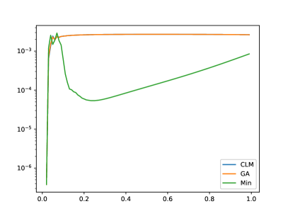
The stability and accuracy of the new methods are interrogated in two numerical tests and the three discrete continuity equations are compared in our third test. The tests employ the finite element method to discretize space, with Taylor-Hood (2/1subscript2subscript1\mathbb{P}_{2}/\mathbb{P}_{1}) elements, [18]. All the stability results proven herein hold for this spatial discretization by essentially the same proofs. The meshes used for both tests are generated using a Delaunay triangulation. The software package FEniCS is used for both experiments [1].

We begin with comparative tests of the adaptive k,ε𝑘𝜀k,\varepsilon, first and second-order method. Both adapt ε𝜀\varepsilon based on unorm𝑢||\nabla\cdot u||. The first-order method accepts the first-order approximation un+11superscriptsubscript𝑢𝑛11u_{n+1}^{1} and adapts the time-step based on EST(1)𝐸𝑆𝑇1EST(1). The second-order method accepts un+1subscript𝑢𝑛1u_{n+1} as the approximation and adapts the time step based on EST(2)𝐸𝑆𝑇2EST(2).

5.1 Test 1: Flow Between Offset Circles

To interrogate stability and accuracy of the GA-method, we present the results of two numerical tests. Pick

Ω={(x,y):x2+y2r12 and (xc1)2+(yc2)2r22},Ωconditional-set𝑥𝑦superscript𝑥2superscript𝑦2superscriptsubscript𝑟12 and superscript𝑥subscript𝑐12superscript𝑦subscript𝑐22superscriptsubscript𝑟22\displaystyle\Omega=\{(x,y):x^{2}+y^{2}\leq r_{1}^{2}\text{ and }(x-c_{1})^{2}+(y-c_{2})^{2}\geq r_{2}^{2}\},
r1=1,r2=0.1,c=(c1,c2)=(12,0),formulae-sequencesubscript𝑟11formulae-sequencesubscript𝑟20.1𝑐subscript𝑐1subscript𝑐2120\displaystyle r_{1}=1,r_{2}=0.1,c=(c_{1},c_{2})=(\frac{1}{2},0),
f=min{t,1}(4y(1x2y2),4x(1x2y2))T, for 0t10.formulae-sequence𝑓𝑡1superscript4𝑦1superscript𝑥2superscript𝑦24𝑥1superscript𝑥2superscript𝑦2𝑇 for 0𝑡10\displaystyle f=\min\{t,1\}(-4y(1-x^{2}-y^{2}),4x(1-x^{2}-y^{2}))^{T},\text{ for }0\leq t\leq 10.

with no-slip boundary conditions on both circles and ν=0.001𝜈0.001\nu=0.001. The finite element discretization has a maximal mesh width of hmax=0.0133,subscript𝑚𝑎𝑥0.0133h_{max}=0.0133, and the flow was solved using the direct solver UMFPACK [8]. For this test, we use fixed tolerances TOLm=TOLc=0.001𝑇𝑂subscript𝐿𝑚𝑇𝑂subscript𝐿𝑐0.001TOL_{m}=TOL_{c}=0.001. The flow (inspired by the extensive work on variants of Couette flow, [12]), driven by a counterclockwise force (with f0𝑓0f\equiv 0 at the outer circle), rotates about (0,0)00(0,0) and interacts with the immersed circle. This induces a von Kármán vortex street which re-interacts with the immersed circle creating more complex structures. There is also a central (polar) vortex that alternately self-organizes then breaks down. Each of these events includes a significant pressure response.

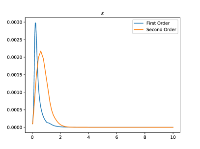
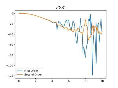
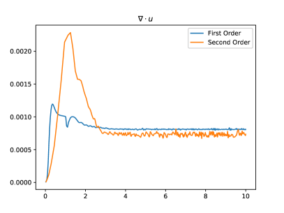
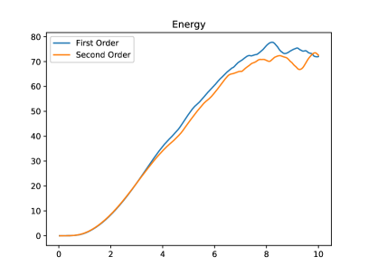
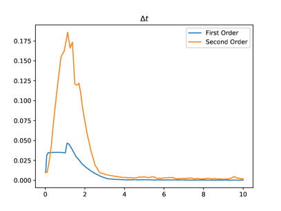
For both approximations we track the evolution of knsubscript𝑘𝑛k_{n} and εnsubscript𝜀𝑛\varepsilon_{n}, the pressure at the origin, the violation of incompressibility, and the algorithmic energy uhn+12+εn+1phn+12superscriptnormsuperscriptsubscript𝑢𝑛12subscript𝜀𝑛1superscriptnormsuperscriptsubscript𝑝𝑛12\|u_{h}^{n+1}\|^{2}+\varepsilon_{n+1}\|p_{h}^{n+1}\|^{2}. These are all depicted in Figure 1 below.
Refer to caption
(A) Timestep evolution
Refer to caption
(B) ε𝜀\varepsilon evolution
Refer to caption
(C) Pressure at the origin
Refer to caption
(D) Divergence evolution
Refer to caption
(E) Energy evolution
Fig. 1: Stability and adaptability results.

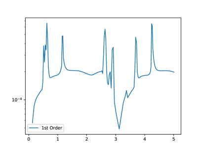
Figure 1A shows that the second-order scheme consistently chooses larger time-steps than the first-order method. The evolution of ε𝜀\varepsilon, in Figure 1B, behaves similarly for both methods once the flow evolves. In testing AC methods pressure initialization often causes irregular, transient spiky behavior near t=0𝑡0t=0 such as in Figures 1A, 1B, 1D.

The behavior of the pressure at the origin, p(0,0;t)𝑝00𝑡p(0,0;t) vs. t𝑡t, is depicted in Figure 1C. To our knowledge, there is no convergence theory for AC methods (or even fully coupled methods) which implies maximum norm convergence for the pressure over significant time intervals and for larger Reynolds numbers. Still, the irregular behavior observed in approximate solutions, while not conforming to a convergence theory, reflects vortex events across the whole domain and is interesting to compare. The profiles of the pressure at the origin are similar for both methods over 0t40𝑡40\leq t\leq 4. For t>4,𝑡4t>4, p(0,0;t)𝑝00𝑡p(0,0;t) for the second-order scheme is less oscillatory. This is surprising because the first-order scheme has more numerical dissipation. The divergence evolution of the schemes also differ in the initial transient of u(t)norm𝑢𝑡||\nabla\cdot u(t)||. After the initial transient, the divergence behavior is similar. It is also possible that the difference in unorm𝑢||\nabla\cdot u|| transients is due to the strategy of εlimit-from𝜀\varepsilon-adaptation being sub-optimal. The model energy of both methods is largely comparable. We note that the model energy depends on the choices of ε𝜀\varepsilon made. Thus model energy is not expected to coincide exactly. Generally, Figures 1D1E behave similarly for both algorithms.

5.2 Test 2: Convergence and Adaptivity

The second numerical test concerns the accuracy and adaptivity of the GA-method. Let Ω=]0,1[2\Omega=]0,1[^{2}, with ν=1𝜈1\nu=1. Consider the exact solution (obtained from [14] and applied to the Navier-Stokes equations)

u=πsint(sin2πysin2πx,sin2πxsin2πy)𝑢𝜋𝑡2𝜋𝑦superscript2𝜋𝑥2𝜋𝑥superscript2𝜋𝑦\displaystyle u=\pi\sin{t}(\sin{2\pi y}\sin^{2}{\pi x},-\sin{2\pi x}\sin^{2}{\pi y})
p=costcosπxsinπy,𝑝𝑡𝜋𝑥𝜋𝑦\displaystyle p=\cos{t}\cos{\pi x}\sin{\pi y},

and consider a discretization of ΩΩ\Omega obtained by 300 nodes on each edge of the square. We proceed by running five experiments, adapting both the first- and second-order schemes using the algorithms above, where the tolerance for the continuity and momentum equations is 10(.25i+3)superscript10.25𝑖310^{-(.25i+3)} for i=0,1,2,3,4𝑖01234i=0,1,2,3,4. To control the size of the timesteps, we require knsubscript𝑘𝑛k_{n} to be chosen such that EST(1)(TOLm/10,TOLm)𝐸𝑆𝑇1𝑇𝑂subscript𝐿𝑚10𝑇𝑂subscript𝐿𝑚EST(1)\in(TOL_{m}/10,TOL_{m}). The solutions were obtained in parallel, utilizing the MUMPS direct solver [2]. To examine convergence, we present in Figure 2 log-log plots of the errors of the pressure and the velocity against the average time-step taken during the test. We also present semilog plots of the evolution of the pressure error and timestep during the final test below. The plots show that the time-step adaptation is working as expected and reducing the velocity error, Figure 2C. Our intuition is that the pressure error is linked to satisfaction of incompressibility; however, Figure 2D indicates convergence with respect to the timestep. In our calculations we did observe the following: If unorm𝑢||\nabla\cdot u|| is, e.g., two orders of magnitude smaller then the tolerance, ε𝜀\varepsilon is rapidly increased to be even 𝒪(1)𝒪1\mathcal{O}(1). At this point the pressure error and violation of incompressibility spike upward and ε𝜀\varepsilon is then cut rapidly. This behavior suggests that a band of acceptable ε𝜀\varepsilon-values should be imposed in the adaptive algorithm.
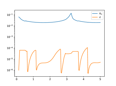
Refer to caption
(A) Timestep and ε𝜀\varepsilon evolution
Refer to caption
(B) Pressure error evolution
Refer to caption
(C) Average timestep vs. velocity error
Refer to caption
(D) Average timestep vs. pressure error
Fig. 2: Accuracy and adaptability results.

To compare the GA, Min method and the scheme introduced in [6], we use the test problem given above in this section with a known exact solution. The results are given in Figure 3 below. Here, we use a mesh with the same density and final time T=1𝑇1T=1. A timestep kn=102subscript𝑘𝑛superscript102k_{n}=10^{-2} is kept constant in this run to highlight differences in the evolution of the variable εnsubscript𝜀𝑛\varepsilon_{n}, which has an initial value ε0=104subscript𝜀0superscript104\varepsilon_{0}=10^{-4}. These tests are preliminary: In them, the min-Method seems preferable in error behavior but yields smaller values and thus less well-conditioned systems. In the evolution of all four quantities, the GA- and the CLM [6] method exhibit near identical behavior. The min-Method, however, forces ε𝜀\varepsilon to be an order of magnitude lower than the values obtained by the other two schemes. This, in turn, forces the divergence to be reduced. Furthermore, both the velocity and pressure errors for the min-Method are smaller than those of the GA- and CLM-Methods.
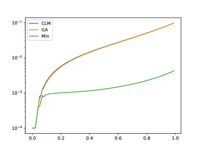
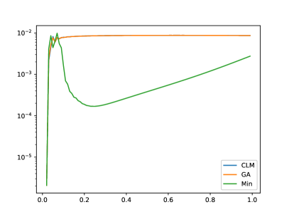
Refer to caption
(A) ε𝜀\varepsilon evolution
Refer to caption
(B) Divergence norm evolution
Refer to caption
(C) Velocity error evolution
Refer to caption
(D) Pressure error evolution
Fig. 3: Comparison between GA, Min, and CLM methods.

6 Conclusions, open problems and future prospects

There are many open problems and algorithmic improvements possible. The doubly adaptive algorithm selected smaller values of ε𝜀\varepsilon than k𝑘k in our tests with the same tolerance for both. A further synthesis of the methods herein with the modular grad-div algorithm of [13] would eliminate any conditioning issues in the linear system arising. Developing doubly adaptive methods of order greater than two (with modular grad-div) is an important step to greater time accuracy. We mention in particular the new embedded family of orders 2,3,4 of [10] as a natural extension. The method of Dahlquist, Liniger and Nevanlinna [7] is unexplored for PDEs, but has promise in CFD because it is A-stable for both increasing and decreasing time-steps. Improved error estimators for the second-order method herein would increase reliability. For AC methods, pressure initialization and damping of nonphysical acoustics are important problems where further progress would be useful.

Open problems. The idea of adapting independently k𝑘k and ε𝜀\varepsilon is promising but new so there are many open problems. These include:

  • Is the ε𝜀\varepsilon-adaptation formula εnew=εold(TOL/u)subscript𝜀𝑛𝑒𝑤subscript𝜀𝑜𝑙𝑑𝑇𝑂𝐿norm𝑢\varepsilon_{new}=\varepsilon_{old}(TOL/||\nabla\cdot u||) improvable? Perhaps the quotient should be to some fractional power. Perhaps adapting ε𝜀\varepsilon should be based of a relative error in unorm𝑢||\nabla\cdot u||, such as u/unorm𝑢norm𝑢||\nabla\cdot u||/||\nabla u||. Analysis of the local (in time) error in unorm𝑢||\nabla\cdot u|| is needed to support an improvement.

  • The ε𝜀\varepsilon-adaptation strategy seems to need preset limits, εmin,εmaxsubscript𝜀subscript𝜀\varepsilon_{\min},\varepsilon_{\max}, to enforce εminεεmaxsubscript𝜀𝜀subscript𝜀\varepsilon_{\min}\leq\varepsilon\leq\varepsilon_{\max}. The preset of εminsubscript𝜀\varepsilon_{\min} is needed because u=0𝑢0\nabla\cdot u=0 cannot be enforced pointwise in many finite element spaces. Finding a reasonable strategy for these presets is an open problem. Similarly, it would be useful to develop a coherent strategy for relating the two tolerances rather than simply picking them to be equal (as herein).

  • Proving convergence to a weak solution of the incompressible NSE of solutions to the continuum analogs of the GA-method and min-Method for variable ε𝜀\varepsilon is an important open problem. In this analysis it is generally assumed that ε(t)0𝜀𝑡0\varepsilon(t)\rightarrow 0 in an arbitrary fashion. A more interesting problem is to link ε(t)𝜀𝑡\varepsilon(t) and unorm𝑢||\nabla\cdot u|| in the analysis. Similarly, an á priori error analysis for variable ε𝜀\varepsilon is an open problem and may yield insights on how the variance of ε(t)𝜀𝑡\varepsilon(t) should be controlled within an adaptive algorithm. The consistency error of the two methods are 𝒪(k+ε)𝒪𝑘𝜀\mathcal{O}(k+\varepsilon) and 𝒪(k2+ε)𝒪superscript𝑘2𝜀\mathcal{O}(k^{2}+\varepsilon), respectively. Energy stability has been proven herein for the first order method and for the constant time-step, second order method. Thus, error estimation while technical, should be achievable.

  • Comprehensive testing of the variable (first or second) order method is an open problem. VSVO methods are the most effective for systems of ODEs but have little penetration in CFD. Testing the relative costs and accuracy of VSVO in CFD is an important problem.

References

  • [1] M. Alnæs, J. Blechta, J. Hake, A. Johansson, B. Kehlet, A. Logg, C. Richardson, J. Ring, M.E. Rognes, G.N. Wells, The FEniCS project version 1.5, Archive of Numerical Software 3 (2015), 9–23.
  • [2] P. Amestoy, I. Duff, J.-Y. L’Excellent, and J. Koster, A fully asynchronous multifrontal solver using distributed dynamic scheduling, SIAM Journal on Matrix Analysis and Applications 23 (2001), 15–41.
  • [3] R.A. Asselin, Frequency filter for time integration, Mon. Weather Review 100(1972), 487–490.
  • [4] G.A. Baker, Galerkin approximations for the Navier-Stokes equations, Technical Report,1976.
  • [5] J. M. Connors, J. Howell, and W. Layton, Decoupled time stepping for a fluid-fluid interaction problem, SIAM J. Numer. Anal. 50 (2012), pp. 1297-1319
  • [6] R.M. Chen, W. Layton, and M. McLaughlin, Analysis of variable step/non-autonomous artificial compression methods, JMFM 21 (2018).
  • [7] G. Dahlquist, W. Liniger and O. Nevanlinna, Stability of two-step methods for variable integration steps , SIAM J. Numer. Anal. 20 (1983), 1071–1085.
  • [8] T. Davis, Direct methods for sparse linear systems, SIAM, vol. 2, 2006.
  • [9] V. DeCaria, W. Layton and M. McLaughlin, A conservative, second-order, unconditionally stable artificial compression method, CMAME 325 (2017), 733–747.
  • [10] V. DeCaria, A. Guzel W. Layton and Yi Li, A new embedded variable stepsize, variable order family of low computational complexity, https://arxiv.org/abs/1810.06670, 2018.
  • [11] V. DeCaria, W. Layton and Haiyun Zhao, Analysis of a low complexity, time-accurate discretization of the Navier-Stokes equations, https://arxiv.org/abs/1810.06705, 2018.
  • [12] C. Egbers and G. Pfister, Physics of rotating fluids, Springer LN in Physics 549 (2018).
  • [13] J. Fiordilino, W. Layton, and Y. Rong, An efficient and modular grad-div stabilization, Computer Methods in Applied Mechanics and Engineering 335 (2018), 327–346.
  • [14] J.-L. Guermond, P. Minev and J. Shen, An overview of projection methods for incompressible flows, Comput. Methods Appl. Mech. Engrg. 195 (2006), 6011–6045.
  • [15] J.-L. Guermond and P. Minev, High-Order Time Stepping for the Incompressible Navier–Stokes Equations, SIAM J. Sci. Comput. 37-6 (2015), A2656-A2681 http://dx.doi.org/10.1137/140975231.
  • [16] J.-L. Guermond and P. Minev, High-order time stepping for the Navier–Stokes equations with minimal computational complexity, JCAM 310 (2017), 92–103.
  • [17] J.-L. Guermond and P. Minev, High-order, adaptive time stepping scheme for the incompressible Navier–Stokes equations, technical report 2018.
  • [18] M.D. Gunzburger, Finite Element Methods for Viscous Incompressible Flows - A Guide to Theory, Practices, and Algorithms, Academic Press, 1989.
  • [19] A. Guzel and W. Layton, Time filters increase accuracy of the fully implicit method, BIT Numerical Mathematics, 58 (2018), 301-315.
  • [20] A. Hay, S. Etienne, D. Pelletier and A. Garon, hp-Adaptive time integration based on the BDF for viscous flows. JCP, 291 (2015), 151-176.
  • [21] J. Hoffman and C. Johnson, Computational turbulent incompressible flow: Applied mathematics: Body and soul 4 (Vol. 4). Springer, Berlin, 2007.
  • [22] H. Johnston and J.-G. Liu, Accurate, stable and efficient Navier-Stokes solvers based on an explicit treatment of the pressure term, JCP 199(2004) 221-259.
  • [23] D.A. Kay, P.M. Gresho, P.M., Griffiths and D.J. Silvester, Adaptive time-stepping for incompressible flow Part II: Navier–Stokes equations. SIAM Journal on Scientific Computing, 32(2010), 111-128.
  • [24] G.M. Kobel’kov, Symmetric approximations of the Navier-Stokes equations, Sbornik: Mathematics. 193(2002), 1027-1047.
  • [25] W. Layton, Y. Li, and C. Trenchea, Recent developments in IMEX methods with time filters for systems of evolution equations, J. Comp. Applied Math. 299 (2016), 50–67.
  • [26] T. Ohwada and P. Asinari, Artificial compressibility method revisited: Asymptotic numerical method for incompressible Navier Stokes equations. J. Comp. Physics, 229:16981723, 2010.
  • [27] A. Prohl, Projection and quasi-compressibility methods for solving the incompressible Navier-Stokes equations, Springer, Berlin, 1997.
  • [28] A. Robert, The integration of a spectral model of the atmosphere by the implicit method, Proc. WMO/IUGG Symposium on NWP, Japan Meteorological Soc. , Tokyo, Japan, pp. 19-24, 1969.
  • [29] J. Shen, On a new pseudocompressibility method for the incompressible Navier-Stokes equations, Appl. Numer. Math. 21 (1996), 71–90.
  • [30] J. Shen, On error estimates of projection methods for the Navier-Stokes equations: First-Order Schemes, SINUM 29(1992) 57-77.
  • [31] J. Shen, On error estimates of higher order projection and penalty-projection schemes for the Navier-Stokes equations, Numer. Math. 62(1992) 49-73.
  • [32] J. Shen, On error estimates of the projection method for the Navier-Stokes equations: second-order schemes,Math. Comp. 65(1996)1039-1065.
  • [33] C. Temperton and A. Staniforth, An efficient two-time level semi-Lagrangian semi-implicit scheme, Q.J.Royal Meteor. Soc. 113(1987),1027-1039.
  • [34] A. Veneziani and U. Villa, ALADINS: An algebraic splitting time-adaptive solver for the incompressible Navier-Stokes equations, JCP 238(2013) 359-375.
  • [35] P.D. Williams, A proposed modification to the Robert-Asselin time filter, Monthly Weather Review, 137(2009), 2538-2546.
  • [36] P.D. Williams, The RAW Filter: An Improvement to the Robert–Asselin Filter in Semi-Implicit Integrations, Mon. Weather Rev., 139 (2011), 1996–2007.
  • [37] L. Yang, S. Badia and R. Codina, A pseudo-compressible variational multiscale solver for turbulent incompressible flows, Comp. Mechanics 58(2016) 1051-1069.
  • [38] R.Kh. Zeytounian, Topics in hyposonic flow theory, Lecture Notes in Physics, Springer, Berlin, 2006.