Measurement of the $e^{+}e^{-}\rightarrow\eta\pi^{+}\pi^{-}$ cross section with the CMD-3 detector at the VEPP-2000 collider

Abstract

The cross section of the process $e^{+}e^{-}\rightarrow\eta\pi^{+}\pi^{-}$ is measured using the data collected with the CMD-$3$ detector at the VEPP-$2000$ collider in the center-of-mass energy range from $1.1$ to $2.0$ GeV. The decay mode $\eta\rightarrow\gamma\gamma$ is used for $\eta$ meson reconstruction in the data sample corresponding to an integrated luminosity of $78.3$ pb^-1. The energy dependence of the $e^{+}e^{-}\rightarrow\eta\pi^{+}\pi^{-}$ cross section is fitted within the framework of vector meson dominance in order to extract the $\Gamma(\rho(1450)\rightarrow e^{+}e^{-})\mathcal{B}(\rho(1450)\rightarrow\eta\pi^{+}\pi^{-})$ and the $\Gamma(\rho(1700)\rightarrow e^{+}e^{-})\mathcal{B}(\rho(1700)\rightarrow\eta\pi^{+}\pi^{-})$ products. Based on conservation of vector current, the analyzed data are used to test the relationship between the $e^{+}e^{-}\rightarrow\eta\pi^{+}\pi^{-}$ cross section and the spectral function in $\tau^{-}\rightarrow\eta\pi^{-}\pi^{0}\nu_{\tau}$ decay. The $e^{+}e^{-}\rightarrow\eta\pi^{+}\pi^{-}$ cross section obtained with the CMD-$3$ detector is in good agreement with the previous measurements.

I Introduction

We report on a study of the process $e^{+}e^{-}\rightarrow\eta\pi^{+}\pi^{-}$ with the CMD-$3$ detector at the VEPP-$2000$ $e^{+}e^{-}$ collider, where $\eta$ mesons are reconstructed using the decay mode $\eta\rightarrow\gamma\gamma$. In the previous experiments it has been shown that this isovector final state is mainly produced through the $\eta\rho(770)$ intermediate mechanism [17, 5]. As a part of the total hadronic cross section, the cross section of the process $e^{+}e^{-}\rightarrow\eta\pi^{+}\pi^{-}$ is interesting for the calculations of the hadronic contribution to the muon anomalous magnetic moment [23, 31, 32]. The $e^{+}e^{-}\rightarrow\eta\pi^{+}\pi^{-}$ cross section data can be also used to study the properties of the $\rho(1450)$ and $\rho(1700)$ resonances, as well as to obtain the hadronic spectral function for the $\tau^{-}\rightarrow\eta\pi^{-}\pi^{0}\nu_{\tau}$ decay and thus test conservation of vector current [25].

The process $e^{+}e^{-}\rightarrow\eta\pi^{+}\pi^{-}$ was studied earlier in several experiments [24, 15, 10, 16, 4, 17, 5, 37, 38]. The most precise measurements of its cross section have been performed at the PEP-II B-factory by the BaBar Collaboration [37].

II Experiment

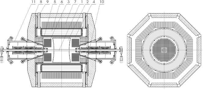
Figure 1: The schematic view of the CMD-3 detector. (1) beam pipe, (2) drift chamber, (3) BGO endcap calorimeter, (4) Z-chamber, (5) superconducting solenoid, (6) liquid xenon calorimeter, (7) CsI barrel calorimeter, (8) iron yoke, (9) liquid He supply, (10) vacuum pumpdown, (11) VEPP-2000 superconducting magnetic lenses.

The data sample has been collected with the CMD-3 detector at the VEPP-$2000$ $e^{+}e^{-}$ collider [21, 34, 1, 2, 41, 42] in $2011$, $2012$ and $2017$ experimental runs. In order to reach the design luminosity in the single-bunch mode, the collider is operated using the round beam technique [18] in the center-of-mass (c.m.) energy range from $0.32$ to $2.0$ GeV. The beam energy was measured using a VEPP-2000 magnetic field in the $2011$ and $2012$ experimental runs [21, 34, 41, 42], and with the backscattering-laser-light system in the $2017$ one [1, 2]. The accuracy of the beam energy measurements is about $3$ MeV in 2011 and about $1$ MeV in 2012, while in 2017 it is better than $0.1$ MeV.

The general-purpose cryogenic magnetic detector CMD-3 has been described in detail elsewhere [33]. The schematic view of the CMD-$3$ detector is shown in Fig. 1. The tracking system of the CMD-$3$ detector consists of a double-layer multiwire proportional Z-chamber [11] and a cylindrical drift chamber [28] with hexagonal cells, which volume is filled with the argon-isobutane gas mixture. Magnetic field of $1.3$ T inside the tracking system is provided by the superconducting solenoid, which surrounds the drift and Z-chambers. The barrel electromagnetic calorimeter is situated outside the superconducting solenoid and consists of two parts. The first part is the liquid xenon calorimeter (a thickness is $5.4X_{0}$, where $X_{0}$ is a radiation length), which allows photon coordinates to be measured with the accuracy of $1$–$2$ mm [14]. The second part is the calorimeter composed of CsI(Tl) and CsI(Na) crystals (a thickness of $8.1X_{0}$). This calorimeter consists of $8$ octants and contains $1152$ counters. The endcap calorimeter [12] consists of two identical endcaps, each containing $340$ BGO crystals with a thickness of $13.4X_{0}$.

III Simulation

The Monte Carlo (MC) simulation of the process $e^{+}e^{-}\rightarrow\eta\pi^{+}\pi^{-}$ has been performed separately at each $e^{+}e^{-}$ energy corresponding to the collected experimental data. It takes into account the $\eta\rho(770)$ intermediate state with the following matrix element:

$$M_{fi}\propto\frac{1}{D(Q_{\pi^{+}\pi^{-}})}\varepsilon_{\alpha\beta\gamma\delta}J^{\alpha}P^{\beta}_{\pi^{+}}P^{\gamma}_{\pi^{-}}P^{\delta}_{\eta},$$ (1)

where $J$ is a lepton current, $P_{\pi^{+}}$, $P_{\pi^{-}}$, $P_{\eta}$ are four-momenta of $\pi^{+}$, $\pi^{-}$ and $\eta$, respectively. $D(Q_{\pi^{+}\pi^{-}})=Q^{2}_{\pi^{+}\pi^{-}}-m^{2}_{\rho(770)}+i\sqrt{Q^{2}_{\pi^{+}\pi^{-}}}\Gamma_{\rho(770)}$ is the inverse propagator of the $\rho(770)$, $m_{\rho(770)}$ and $\Gamma_{\rho(770)}$ are the mass and the width of the $\rho(770)$, respectively, and $Q_{\pi^{+}\pi^{-}}=P_{\pi^{+}}+P_{\pi^{-}}$ is its four-momentum. To take into account the initial-state radiation according to works [36, 8], the simulation is done in two iterations. In the first iteration, the cross section of the process $e^{+}e^{-}\rightarrow\eta\pi^{+}\pi^{-}$ measured with BaBar is used to simulate ISR photons, while in the second one the cross section measured with the CMD-3 obtained in the first iteration is employed for this purpose. For a simulation of various multihadronic backgrounds the MHG$2000$ generator specially developed for experiments at CMD-$3$ has been used [20]. The interactions of the generated particles with the detector and its response are implemented using the Geant$4$ toolkit [9].

IV Event selection

To select $e^{+}e^{-}\rightarrow\eta\pi^{+}\pi^{-}$ event candidates, the following criteria are used. To begin with, events are selected with two oppositely charged particles originating from the beam interaction region. In addition, it is required that the selected events contain at least two photons with energies greater than $50$ MeV to suppress background processes with low-energy photons. Also excluded are photons, which pass through the BGO crystals closest to the beam axis. For each selected event all photon pairs are considered and a kinematic fit is performed within the $e^{+}e^{-}\rightarrow\pi^{+}\pi^{-}\gamma\gamma$ hypothesis using the constraints of energy-momentum conservation and requiring all particles to originate from a common vertex. The photons from the pair corresponding to the smallest chi-square of the kinematic fit, $\chi^{2}_{\pi^{+}\pi^{-}\gamma\gamma}$, are considered as candidates for the photons from the $\eta\rightarrow\gamma\gamma$ decay. Only events with the fit quality $\chi^{2}_{\pi^{+}\pi^{-}\gamma\gamma}<30$ are used to obtain two-photon invariant mass spectra, discussed in Sec. V. The same condition was imposed on the chi-square of the kinematic fit to obtain the distributions discussed in Sec. VI.

The $\chi^{2}_{\pi^{+}\pi^{-}\gamma\gamma}$ distribution obtained using the whole $e^{+}e^{-}\rightarrow\eta\pi^{+}\pi^{-}$ data sample is shown in Fig. 2. The corresponding $\chi^{2}$ distribution for simulated $e^{+}e^{-}\rightarrow\eta\pi^{+}\pi^{-}$ events is also shown. The contributions to the $\chi^{2}_{\pi^{+}\pi^{-}\gamma\gamma}$ distribution for simulated $e^{+}e^{-}\rightarrow\eta\pi^{+}\pi^{-}$ events at each c.m. energy are proportional to $\sigma(e^{+}e^{-}\rightarrow\eta\pi^{+}\pi^{-}){L_{\rm int}}$, where $\sigma(e^{+}e^{-}\rightarrow\eta\pi^{+}\pi^{-})$ is the cross section of the process $e^{+}e^{-}\rightarrow\eta\pi^{+}\pi^{-}$ and $L_{\rm int}$ is the integrated luminosity. Efficiency corrections discussed in Sec. VII are also taken into account to obtain the $\chi^{2}_{\pi^{+}\pi^{-}\gamma\gamma}$ distribution for the MC data sample. In addition, these efficiency corrections are taken into account to obtain other MC distributions given in this paper. The $\chi^{2}_{\pi^{+}\pi^{-}\gamma\gamma}$ distributions have been obtained using all selection criteria above except that on $\chi^{2}$ of the kinematic fit. The remaining background (Sec. V) is subtracted using sidebands in two-photon invariant mass spectra (Sec. VI). The histogram for simulated $e^{+}e^{-}\rightarrow\eta\pi^{+}\pi^{-}$ events is normalized according to the ratio of the number of simulated and experimental data events at $\chi^{2}<30$. There is some disagreement between $\chi^{2}$ distributions for the experimental data and simulated $e^{+}e^{-}\rightarrow\eta\pi^{+}\pi^{-}$ events. To address this disagreement, a corresponding correction to the detection efficiency is applied, which is discussed in Sec. VII.

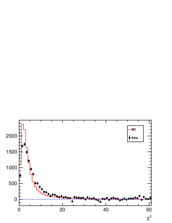
Figure 2: $\chi^{2}$ of the kinematic fit under the $e^{+}e^{-}\rightarrow\pi^{+}\pi^{-}\gamma\gamma$ hypothesis (points with error bars) and simulated $e^{+}e^{-}\rightarrow\eta\pi^{+}\pi^{-}$ events (histogram) from the energy range $\sqrt{s}=1.3$–$1.8$ GeV.

V $\boldsymbol{\eta\pi^{+}\pi^{-}}$ event yield and background subtraction

To determine the $\eta\pi^{+}\pi^{-}$ yield the two-photon invariant mass spectrum at each $e^{+}e^{-}$ energy in the experimental data is fit with a sum of signal and background distributions. The shape of the background distribution has been described using a first-order polynomial. The shape of the signal distribution has been fixed from the $e^{+}e^{-}\rightarrow\eta\pi^{+}\pi^{-}$ MC simulation using a function, which is a linear combination of three Gaussian distributions.

To take into account a difference in the two-photon mass resolution and the $\eta$-meson peak position between the data and MC, two additional parameters, $\Delta{m}$ and $\Delta\sigma^{2}$, are introduced. Here $\Delta{m}$ is the mass shift of the signal distribution as a whole and $\Delta\sigma^{2}$ is the square of the two-photon mass resolution correction, which is added to the variance, $\sigma^{2}$, of each Gaussian distribution from the signal function.

The free parameters of the fit to the two-photon invariant mass spectrum are the number of signal events, the mass shift of the signal, the square of the two-photon mass resolution correction and background distribution parameters. The total number of the fitted $e^{+}e^{-}\rightarrow\eta\pi^{+}\pi^{-}$ events is $13426\pm 206$. An example of the two-photon invariant mass spectrum for $e^{+}e^{-}\rightarrow\eta\pi^{+}\pi^{-}$ event candidates at $\sqrt{s}=1.5$ GeV is shown in Fig. 3. The $e^{+}e^{-}\rightarrow\eta\pi^{+}\pi^{-}$ event yields for different c.m. energy points are listed in Table 1. No excess of signal events over background is observed at c.m. energies below $1.24$ GeV.

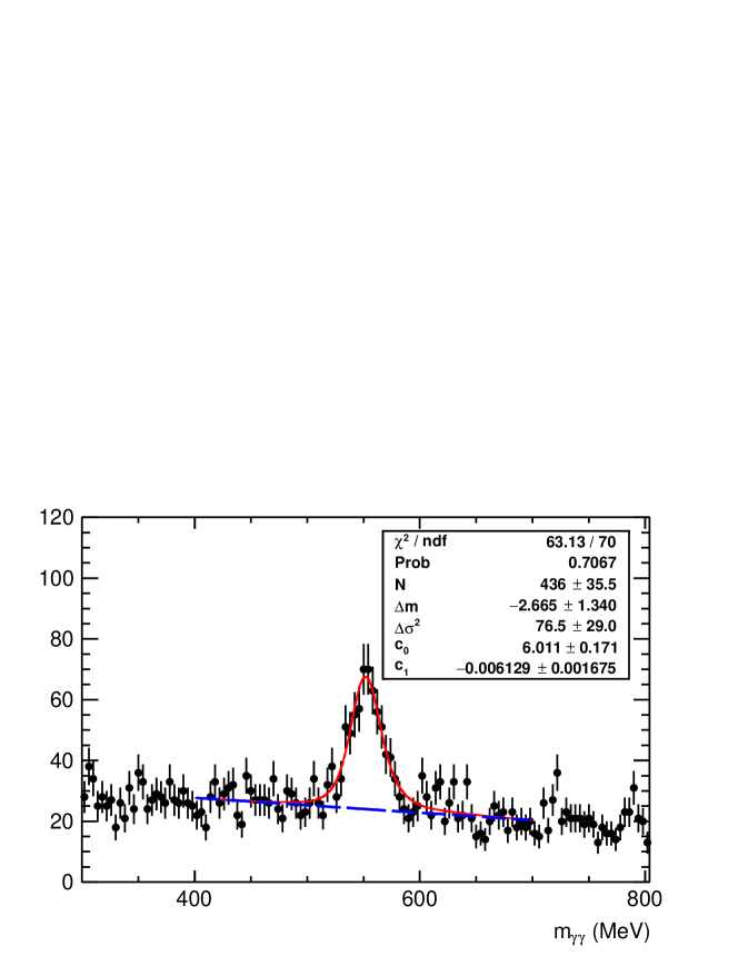
Figure 3: Two-photon invariant mass spectrum for the experimental data events (points with error bars) at $\sqrt{s}=1.5$ GeV fitted with the function (solid curve), which contains the signal and background (dashed curve) contributions.

The main background source for the studied process is that with four final pions, $e^{+}e^{-}\rightarrow\pi^{+}\pi^{-}\pi^{0}\pi^{0}$. Events of this process are partially suppressed by selection criteria and do not have a peak at the $\eta$-meson mass. The sources of the peaking background, the processes $e^{+}e^{-}\rightarrow\eta K^{+}K^{-}$ and $e^{+}e^{-}\rightarrow\eta\pi^{+}\pi^{-}\pi^{0}$, are strongly suppressed by selection criteria. The contributions of these processes have been estimated using MC simulation and corresponding cross sections measured in Ref. [16] and Ref. [13], respectively. The contribution of each process is found to be less than $0.1\%$ and neglected.

VI Internal structure of the $\boldsymbol{\eta\pi^{+}\pi^{-}}$

The $\pi^{+}\pi^{-}$ invariant mass spectra for the whole $e^{+}e^{-}\rightarrow\eta\pi^{+}\pi^{-}$ data sample and simulated $e^{+}e^{-}\rightarrow\eta\pi^{+}\pi^{-}$ events have been obtained as a difference between the $\pi^{+}\pi^{-}$ mass spectrum with $500\;{\rm MeV}<m_{\gamma\gamma}<600\;{\rm MeV}$ and the spectrum for events from sidebands ($400\;{\rm MeV}<m_{\gamma\gamma}<470\;{\rm MeV}$ and $630\;{\rm MeV}<m_{\gamma\gamma}<700\;{\rm MeV}$) divided by a normalization factor of $1.4$. The $\pi^{+}\pi^{-}$ invariant mass spectra for the whole $e^{+}e^{-}\rightarrow\eta\pi^{+}\pi^{-}$ data and simulated $e^{+}e^{-}\rightarrow\eta\pi^{+}\pi^{-}$ events are shown in Fig. 4. Points with error bars correspond to the $\pi^{+}\pi^{-}$ invariant mass distribution for the whole $e^{+}e^{-}\rightarrow\eta\pi^{+}\pi^{-}$ data. The solid histogram corresponds to the $\pi^{+}\pi^{-}$ invariant mass spectrum for simulated $e^{+}e^{-}\rightarrow\eta\pi^{+}\pi^{-}$ events. The $\rho(770)$ signal is seen in both distributions. The contributions to the $\pi^{+}\pi^{-}$ invariant mass spectrum for simulated $e^{+}e^{-}\rightarrow\eta\pi^{+}\pi^{-}$ events at each c.m. energy are proportional to $\sigma(e^{+}e^{-}\rightarrow\eta\pi^{+}\pi^{-}){L_{\rm int}}$.

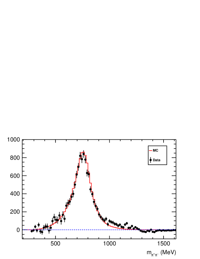
Figure 4: $\pi^{+}\pi^{-}$ invariant mass spectra for the experimental data (points with error bars) and simulated $e^{+}e^{-}\rightarrow\eta\pi^{+}\pi^{-}$ events (histogram) from the energy range $\sqrt{s}=1.3$–$1.8$ GeV. The simulation uses a model of the $\eta\rho(770)$ intermediate state.

Since $\pi^{+}\pi^{-}$ spectra from data and simulation are very similar, we can make a conclusion that the $\eta\rho(770)$ intermediate mechanism assumed in simulation gives indeed the dominant contribution to the internal structure of the $\eta\pi^{+}\pi^{-}$ final state.

The distributions of the $\eta$-meson polar angle, $\theta_{\eta}$, for $e^{+}e^{-}\rightarrow\eta\pi^{+}\pi^{-}$ data and simulated $e^{+}e^{-}\rightarrow\eta\pi^{+}\pi^{-}$ events have been obtained in the same way as the $\pi^{+}\pi^{-}$ invariant mass distributions and are shown in Fig. 5. This distribution is expected to be proportional to $1+\cos^{2}\theta_{\eta}$ in a model of the $\eta\rho$ intermediate state, but the obtained one has a different shape because of the detector response.

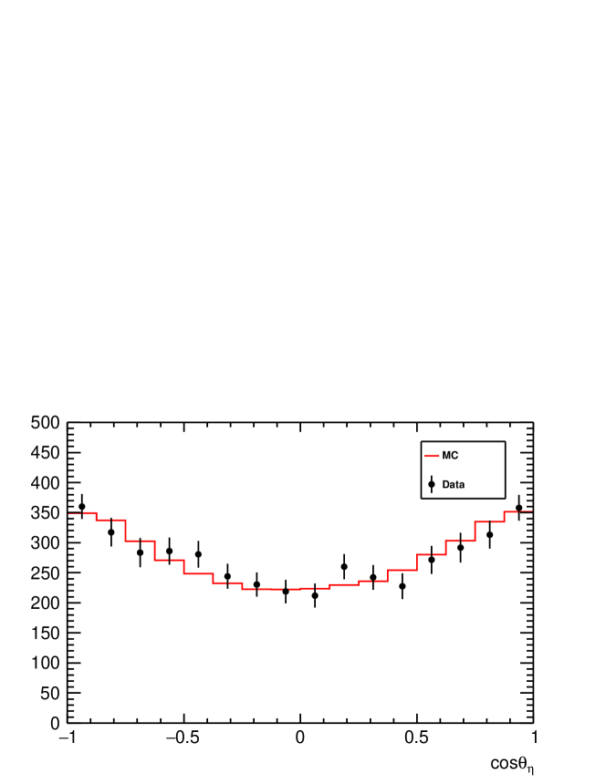
Figure 5: $\cos\theta_{\eta}$ distribution for the experimental data (points with error bars) and simulated $e^{+}e^{-}\rightarrow\eta\pi^{+}\pi^{-}$ events (histogram) in the energy range $\sqrt{s}=1.3$–$1.8$ GeV. Simulation uses a model of the $\eta\rho(770)$ intermediate state.

The $\theta_{\eta}$ distributions for the whole $e^{+}e^{-}\rightarrow\eta\pi^{+}\pi^{-}$ data and for simulated $e^{+}e^{-}\rightarrow\eta\pi^{+}\pi^{-}$ events are shown by points with error bars and by a solid histogram, respectively.

VII Detection efficiency

The detection efficiency for the process $e^{+}e^{-}\rightarrow\eta\pi^{+}\pi^{-}$ has been found from corresponding MC simulation using the following formula:

$$\varepsilon_{\rm MC}=\frac{N^{\prime}_{\rm MC}}{N_{\rm MC}},$$ (2)

where $N_{\rm MC}$ is the initial number of $e^{+}e^{-}\rightarrow\eta\pi^{+}\pi^{-}$ events generated with the MC simulation and $N^{\prime}_{\rm MC}$ is the number of $e^{+}e^{-}\rightarrow\eta\pi^{+}\pi^{-}$ events extracted from the fit to the two-photon invariant mass spectrum.

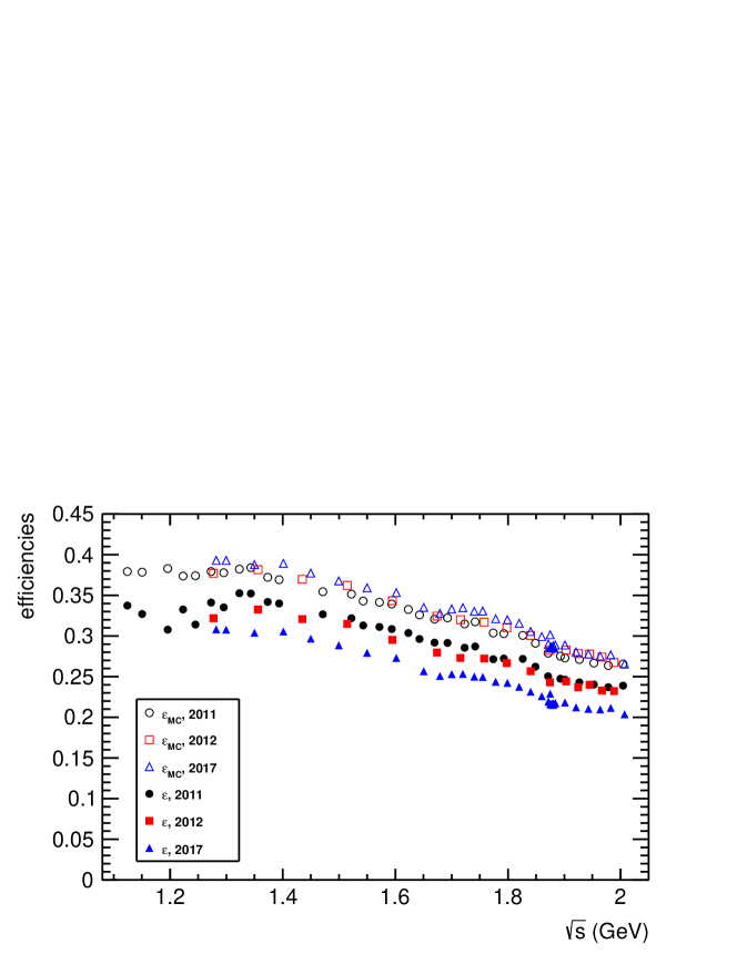
Figure 6: The $e^{+}e^{-}\rightarrow\eta\pi^{+}\pi^{-}$ detection efficiencies for $2011$, $2012$ and $2017$ data samples. The $e^{+}e^{-}\rightarrow\eta\pi^{+}\pi^{-}$ Monte Carlo detection efficiencies are indicated with empty markers while those with corrections with filled markers.

To take into account the difference between the experimental data and the simulation, a set of corrections is applied to the detection efficiency found from the $e^{+}e^{-}\rightarrow\eta\pi^{+}\pi^{-}$ MC simulation. The corrected detection efficiency has been calculated using the following formula:

$$\varepsilon=\varepsilon_{\rm MC}(1+\delta_{\rm trigg})(1+\delta_{\chi^{2}})(1+\delta_{\pi})(1+\delta_{\gamma}),$$ (3)

where $\delta_{\rm trigg}$ is the correction for trigger, $\delta_{\pi}$ is the correction for charged pions, $\delta_{\gamma}$ is the correction for photons and $\delta_{\chi^{2}}$ is the correction, which takes into account a difference between the $\chi^{2}$ value of the kinematic fit distributions in data and the $e^{+}e^{-}\rightarrow\eta\pi^{+}\pi^{-}$ MC simulation. The energy dependence of the MC and corrected detection efficiencies is shown in Fig. 6.

Events are recorded when a signal from at least one of the two independent trigger systems is detected. One of these systems, the charged trigger, uses information from the tracking system only, while the second one, referred to as the neutral trigger, is based on information from the electromagnetic calorimeter only. The efficiencies of charged, $\varepsilon_{\rm CT}$, and neutral, $\varepsilon_{\rm NT}$, triggers can be calculated using the following relation:

$$\varepsilon_{\rm CT}=\frac{\rm N_{\rm CN}}{N_{\rm CN}+N_{\rm N}},$$ (4)

$$\varepsilon_{\rm NT}=\frac{N_{\rm CN}}{N_{\rm CN}+N_{\rm C}},$$

where $N_{\rm CN}$ is the number of events with the simultaneous signals from the charged and neutral triggers, $N_{\rm C}$ is the number of events with signals from the charged trigger only and $N_{\rm N}$ is the number of events with signals from the neutral one only. The trigger efficiency correction, $\delta_{\rm trigg}$, can be calculated using the trigger efficiencies in the following way:

$$\delta_{\rm trigg}=-(1-\varepsilon_{\rm CT})(1-\varepsilon_{\rm NT}).$$ (5)

The typical values of the trigger efficiency correction at $\sqrt{s}>1.35$ GeV are about $(-0.9\pm 0.1)\%$ and $(-1.0\pm 0.1)\%$ for the $2011$ and $2012$ data samples, respectively, while at $\sqrt{s}\leq 1.35$ GeV they are $(-3.8\pm 0.9)\%$ and $(-3.4\pm 0.7)\%$. The typical value of the trigger efficiency correction for the $2017$ data sample is $(-0.58\pm 0.06)\permil$.

The correction, which takes into account a difference between the $\chi^{2}$ value of the kinematic fit distributions for the experimental data and the simulated $e^{+}e^{-}\rightarrow\eta\pi^{+}\pi^{-}$ events, has been calculated using the numbers of $e^{+}e^{-}\rightarrow\eta\pi^{+}\pi^{-}$ events in two statistically independent regions $\chi^{2}_{\pi^{+}\pi^{-}\gamma\gamma}<30$ and $30\leq\chi^{2}_{\pi^{+}\pi^{-}\gamma\gamma}<50$. An additional selection criterion $N_{\gamma}=2$ is also used, where $N_{\gamma}$ is the number of photons that are candidates for the $\eta$ decay photons. All other selection criteria are the same as described in Sec. IV. The correction is given by the following equation:

$$\delta_{\chi^{2}}=1-(1+\Delta N/N)_{\rm data}/(1+\Delta N/N)_{\rm MC},$$ (6)

where $N$ is the number of events in the region $\chi^{2}_{\pi^{+}\pi^{-}\gamma\gamma}<30$ and $\Delta N$ is the number of events in the region $30<\chi^{2}_{\pi^{+}\pi^{-}\gamma\gamma}<50$. The numbers $N$ and $\Delta N$ are found using the $m_{\gamma\gamma}$ spectrum fitting procedure described in the Sec. V. The corresponding detection efficiency corrections, $\delta_{\chi^{2}}$’s, are $(-1.6\pm 0.7)\%$, $(-3.4\pm 1.1)\%$ and $(-3.3\pm 0.8)\%$ for the $2011$, $2012$ and $2017$ data samples, respectively.

The charged-pion detection efficiency correction, $\delta_{\pi}$, has been calculated using the following relation:

$$1+\delta_{\pi}=\sum\Big{(}N^{\rm data}_{\pi^{+}}(\theta_{\pi^{+}})/N^{\rm MC}_{\pi^{+}}(\theta_{\pi^{+}})\Big{)}\Big{(}N^{\rm data}_{\pi^{-}}(\theta_{\pi^{-}})/N^{\rm MC}_{\pi^{-}}(\theta_{\pi^{-}})\Big{)}/N_{\rm MC},$$ (7)

where the sum is taken over events from the $e^{+}e^{-}\rightarrow\eta\pi^{+}\pi^{-}$ MC simulation, $N_{\rm MC}$ is the number of simulated $e^{+}e^{-}\rightarrow\eta\pi^{+}\pi^{-}$ events, $N_{\pi^{\pm}}(\theta_{\pi^{\pm}})$ is the number of $\pi^{\pm}$ tracks with the polar angle equal to $\theta_{\pi^{\pm}}$ in the case, when the second track hits the barrel part of the electromagnetic calorimeter. The superscripts $\rm data$ and $\rm MC$ correspond to the experimental and simulated $e^{+}e^{-}\rightarrow\eta\pi^{+}\pi^{-}$ events. The $N^{\rm MC}_{\pi^{\pm}}(\theta_{\pi^{\pm}})$ distribution is normalized to the number of events in the $N^{\rm data}_{\pi^{\pm}}(\theta_{\pi^{\pm}})$ distribution inside the polar angle region corresponding to the barrel part of the calorimeter. Since the reconstruction efficiency for the second track is close to $99\%$ [35], the ratio of the number of events $N^{\rm data}_{\pi^{\pm}}(\theta_{\pi^{\pm}})/N^{\rm MC}_{\pi^{\pm}}(\theta_{\pi^{\pm}})$ is close to the ratio $\varepsilon^{\rm data}_{\pi^{\pm}}(\theta_{\pi^{\pm}})/\varepsilon^{\rm MC}_{\pi^{\pm}}(\theta_{\pi^{\pm}})$, where $\varepsilon_{\pi^{\pm}}$ is the $\pi^{\pm}$ reconstruction efficiency. The typical values of this correction are about $(-6\pm 6)\%$, $(-9\pm 6)\%$ and $(-20\pm 4)\%$ for the $2011$, $2012$ and $2017$ data samples, respectively.

The photon detection efficiency correction, $\delta_{\gamma}$, has been calculated using the ratio of the reconstruction efficiencies of photons in data and simulation, $\varepsilon^{\rm data}_{\gamma}(\theta)/\varepsilon^{\rm MC}_{\gamma}(\theta)$:

$$1+\delta_{\gamma}=\sum\Big{(}\varepsilon^{\rm data}_{\gamma}(\theta_{\gamma_{1}})/\varepsilon^{\rm MC}_{\gamma}(\theta_{\gamma_{1}})\Big{)}\Big{(}\varepsilon^{\rm data}_{\gamma}(\theta_{\gamma_{2}})/\varepsilon^{\rm MC}_{\gamma}(\theta_{\gamma_{2}})\Big{)}/N_{\rm MC},$$ (8)

where the sum is taken over events from the $e^{+}e^{-}\rightarrow\eta\pi^{+}\pi^{-}$ MC simulation. The typical value of this correction is about $(-0.8\pm 0.2)\%$ for the $2011$, $2012$ and $2017$ data samples. The ratio of the photon reconstruction efficiencies for the experimental data and the simulated events, $\varepsilon^{\rm data}_{\gamma}(\theta)/\varepsilon^{\rm MC}_{\gamma}(\theta)$, has been found using events of the process $e^{+}e^{-}\rightarrow\pi^{+}\pi^{-}\pi^{0}$. Photon reconstruction efficiencies for both data and simulated $e^{+}e^{-}\rightarrow\pi^{+}\pi^{-}\pi^{0}$ events have been calculated as the following ratio:

$$\varepsilon_{\gamma}(\theta)=\frac{N^{\gamma}_{2}}{N^{\gamma}_{1}+N^{\gamma}_{2}},$$ (9)

where $N^{\gamma}_{1}$ is the number of events where only one photon has been detected in the barrel part of the calorimeter and $N^{\gamma}_{2}$ is the number of events with two photons detected: one of them in the barrel part of the calorimeter and the second one in the polar angle $\theta$.

VIII Results and discussion

Table 1: The c.m. energy ($\sqrt{s}$), the $e^{+}e^{-}\rightarrow\eta\pi^{+}\pi^{-}$ Born cross section ($\sigma_{\rm B}$), number of selected signal events ($N$), detection efficiency ($\varepsilon$), integrated luminosity ($L_{\rm int}$).

$\sqrt{s}$, GeV	$\sigma_{\rm B}$, nb	$N$	$\varepsilon$	$L_{\rm int}$, nb-1	$\sqrt{s}$, GeV	$\sigma_{\rm B}$, nb	$N$	$\varepsilon$	$L_{\rm int}$, nb-1
$\slum$

Table 2: The $e^{+}e^{-}\rightarrow\eta\pi^{+}\pi^{-}$ Born cross section ($\sigma_{\rm B}$) at combined c.m. energies ($\sqrt{s}$).

$\sqrt{s}$, GeV	$\sigma_{\rm B}$, nb	$\sqrt{s}$, GeV	$\sigma_{\rm B}$, nb	$\sqrt{s}$, GeV	$\sigma_{\rm B}$, nb
$\tcsec$

The visible cross section at each c.m. energy has been calculated using the following formula:

$$\sigma_{\rm vis}=\frac{N}{L_{\rm int}},$$ (10)

where $N$ is the $e^{+}e^{-}\rightarrow\eta\pi^{+}\pi^{-}$ yield and $L_{\rm int}$ is an integrated luminosity. The integrated luminosity at each c.m. energy has been measured using the $e^{+}e^{-}\rightarrow e^{+}e^{-}$ events [40]. The visible and Born cross sections are related by the following equation [36]:

$$\sigma_{\rm vis}(s)=\int\limits^{x_{0}}_{0}dx\;\sigma_{\rm B}(s(1-x))\varepsilon(x,s)F(x,s),$$ (11)

$$x_{0}=1-(2m_{\pi}+m_{\eta})^{2}/s,$$

where $\sigma_{\rm vis}$ and $\sigma_{\rm B}$ are the visible and Born cross sections, respectively. Here $F(x,s)$ is the initial-state radiation (ISR) kernel function, $\varepsilon(x,s)$ is the detection efficiency, which depends on the fraction of energy carried away by an ISR photon, $m_{\pi}$ and $m_{\eta}$ are masses of the $\pi$ meson and $\eta$ meson, respectively. The detection efficiency for events of the $e^{+}e^{-}\rightarrow\eta\pi^{+}\pi^{-}$ MC simulation at each c.m. energy can be written in the following form:

$$\varepsilon(s)=\frac{\int\limits^{x_{0}}_{0}dx\;\sigma_{\rm B}(s(1-x))\varepsilon(x,s)F(x,s)}{\int\limits^{x_{0}}_{0}dx\;\sigma_{\rm B}(s(1-x))F(x,s)}.$$ (12)

Eq. (12) allows us to rewrite the Eq. (11) in terms of the detection efficiency at each c.m. energy:

$$\sigma_{\rm vis}(s)=\varepsilon(s)\int\limits^{x_{0}}_{0}dx\;\sigma_{\rm B}(s(1-x))F(x,s).$$ (13)

The Born cross section at each c.m. energy in data has been found by solving this integral equation. For this goal, the unknown Born cross section has been interpolated with first-order polynomials from one c.m. energy point to the next one, so the coefficients of the interpolation polynomials linearly depend on the Born cross section at each c.m. energy. Since the integral in Eq. (13) can be calculated at each c.m. energy after the interpolation procedure, we can rewrite Eq. (13) as follows:

$$\vec{\sigma}_{\rm vis}=\mathcal{A}\vec{\sigma}_{\rm B},$$ (14)

$$\vec{\sigma}_{\rm B}=\mathcal{A}^{-1}\vec{\sigma}_{\rm vis},$$

where $\vec{\sigma}_{\rm vis}=(\sigma_{\rm vis}(s_{1}),\sigma_{\rm vis}(s_{2}),...,\sigma_{\rm vis}(s_{n}))$ is the vector composed of visible cross sections at each c.m. energy, $\mathcal{A}$ is the matrix of the integral operator from Eq. (13), and $\vec{\sigma}_{\rm B}=(\sigma_{\rm B}(s_{1}),\sigma_{\rm B}(s_{2}),...,\sigma_{\rm B}(s_{n}))$ is the vector of numerical solutions for Born cross sections at each c.m. energy. The first c.m. energy point used in the cross section interpolation equals the $e^{+}e^{-}\rightarrow\eta\pi^{+}\pi^{-}$ threshold ($\sqrt{s}=2m_{\pi}+m_{\eta}$). The Born cross section and its uncertainty at this point are equal to zero. The inverse error matrix [29] for the Born cross section can be calculated using the following formula:

$$\mathcal{M}=\mathcal{A}^{T}\Lambda\mathcal{A},$$ (15)

where $\Lambda$ is a diagonal inverse error matrix for the visible cross section. The c.m. energy, $e^{+}e^{-}\rightarrow\eta\pi^{+}\pi^{-}$ Born cross section, $e^{+}e^{-}\rightarrow\eta\pi^{+}\pi^{-}$ yield, detection efficiency and integrated luminosity are listed in Table 1.

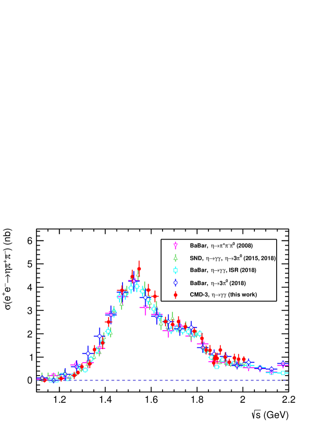
Figure 7: Born cross section for $e^{+}e^{-}\rightarrow\eta\pi^{+}\pi^{-}$ measured at the CMD-3, SND and BaBar. The vertical errors for the Born cross section measured at the CMD-3 correspond to square roots of the error matrix diagonal elements. The close points of the cross section measured with the CMD-3 detector are combined together.

In order to compare the result of the $e^{+}e^{-}\rightarrow\eta\pi^{+}\pi^{-}$ cross section measurement with the previous measurements, we combine the close c.m. energy points in the cross section measured with the CMD-3. The corresponding energy dependence of the $e^{+}e^{-}\rightarrow\eta\pi^{+}\pi^{-}$ Born cross section is shown in Fig. 7. The $e^{+}e^{-}\rightarrow\eta\pi^{+}\pi^{-}$ cross section values at the combined c.m. energy points are also listed in Table 2.

The total systematic uncertainty of the Born cross section is about $6.0\%$ and consists of the contributions from the following sources: the detection efficiency ($5.7\%$), the uncertainty of the ISR correction [36] ($0.1\%$), the uncertainty related with the FSR influence on the detection efficiency ($0.5\%$), the uncertainty on the integrated luminosity ($1\%$), and the uncertainty of the Born cross section numerical calculation ($1\%$). The systematic uncertainty on the detection efficiency includes the following contributions:

• trigger efficiency,

• the requirement on $\chi^{2}$ of the kinematic fit,

• charged pion reconstruction efficiency,

• photon reconstruction efficiency,

• use of the $e^{+}e^{-}\rightarrow\eta\pi^{+}\pi^{-}$ cross section measured with BaBar for MC simulation of the studied process.

The trigger efficiency uncertainty ($0.1$–$0.9\%$) has been estimated as the error of the fit assuming a constant function for the energy dependence of the trigger efficiency correction, $\delta_{\rm trigg}$.

The uncertainty related to the requirement on $\chi^{2}$ of the kinematic fit ($1.1\%$) has been estimated as the error of $\delta_{\chi^{2}}$ obtained using Eq. (6) and two statistically independent $\chi^{2}$ regions, $\chi^{2}<30$ and $30<\chi^{2}<50$.

The uncertainty of the reconstruction efficiency for charged pions ($5.6\%$) has been estimated as the maximum uncertainty for all c.m. energy points given by the uncertainty propagation formula, applied to Eq. (7).

The uncertainty of the reconstruction efficiency for photons ($0.2\%$) has been estimated as the maximum uncertainty for all c.m. energy points given by the uncertainty propagation formula, applied to Eq. (8).

The uncertainty due to use of the $e^{+}e^{-}\rightarrow\eta\pi^{+}\pi^{-}$ cross section measured with BaBar to simulate ISR has been estimated as the relative difference of detection efficiencies in cases of using $e^{+}e^{-}\rightarrow\eta\pi^{+}\pi^{-}$ cross sections measured with BaBar and CMD-3 in MC simulation. The value of this uncertainty ($0.4\%$) appears to be less than its statistical error ($1.2\%$) and is neglected.

The uncertainty related to the shape of the background distribution in two-photon invariant mass spectra has been estimated as the relative difference between the $e^{+}e^{-}\rightarrow\eta\pi^{+}\pi^{-}$ yields, $(N_{2}-N_{1})/N_{1}=(0.5\pm 1.4)\%$, found from the fit to two-photon invariant mass spectra using two different background distribution functions. The first function is a first-order polynomial, the second one is the background distribution taken from multihadron MC simulation [20]. The difference between the $e^{+}e^{-}\rightarrow\eta\pi^{+}\pi^{-}$ yields corresponding to these background hypotheses is found to be statistically insignificant and neglected.

The uncertainty related with the FSR influence on the detection efficiency has been estimated using the PHOTOS++ package [22, 27]. To obtain this uncertainty, the detection efficiencies for two kinds of the $e^{+}e^{-}\rightarrow\eta\pi^{+}\pi^{-}$ MC simulations have been compared at several c.m. energy points. The first kind of $e^{+}e^{-}\rightarrow\eta\pi^{+}\pi^{-}$ MC simulation does not take FSR into account and is described in Sec. III. The second kind of the $e^{+}e^{-}\rightarrow\eta\pi^{+}\pi^{-}$ MC simulation is the same as the first one, but it also takes FSR into account. It has been found that the upper limit on the corresponding uncertainty is $0.5\%$.

The uncertainty of the Born cross section numerical calculation has been estimated using the following formula:

$$\sigma_{\rm calc}=|(\mathcal{A}^{-1}\sigma^{\rm fit}_{\rm vis}-\sigma^{\rm VMD}_{\rm B})/\sigma^{\rm VMD}_{\rm B}|,$$ (16)

where the matrix $\mathcal{A}$ has been taken from Eq. (14), $\sigma^{\rm fit}_{\rm vis}$ is the fit of the visible cross section in the vector meson dominance model (VMD), $\sigma^{\rm VMD}_{\rm B}$ is the VMD parametrization of the Born cross section obtained form the fit of the visible cross section. The visible cross section has been fitted using Eq. (13) and VDM parametrization of the Born cross section in three different ways, discussed below. The obtained uncertainty depends on c.m. energy in the following way:

$$\sigma_{\rm calc}=\begin{cases}1.0\%,\;\sqrt{s}\leq 1.35\;{\rm GeV}\\ 0.2\%,\;1.35\;{\rm GeV}<\sqrt{s}\leq 2.01\;{\rm GeV}\end{cases},$$ (17)

where a relatively big uncertainty at c.m. energies $\sqrt{s}\leq 1.35$ GeV is due to the unknown threshold behavior of the cross section.

The sources of the systematic uncertainty and their contributions are listed in Table 3.

Table 3: The sources of the systematic uncertainty.

Source	Uncertainty, $\%$
	$\sqrt{s}\leq 1.35$ GeV	$\sqrt{s}>1.35$ GeV
$\chi^{2}$ selection criterion	$1.1$
Reconstruction of charged pions	$5.6$
Photon reconstruction	$0.2$
Luminosity	$1.0$
ISR correction	$0.1$
FSR	$0.5$
Trigger efficiency	$0.9$	$0.1$
Uncertainty of the Born cross section numerical calculation	1.0	0.2
Total uncertainty	$6.0$

The function used for the parametrization of the $e^{+}e^{-}\rightarrow\eta\pi^{+}\pi^{-}$ Born cross section in the VMD model contains contributions of several isovector resonances $\rho(770)$, $\rho(1450)$, $\rho(1700)$ that decay to the $\eta\rho(770)$ final state [6, 7] (an isoscalar one is suppressed by G-parity conservation):

$$\sigma_{B}(s)=\frac{4\alpha^{2}}{3s\sqrt{s}}\mathcal{I}(s)|\mathcal{F}(s)|^{2},$$ (18)

$$\mathcal{I}(s)=\displaystyle\int\limits_{4m_{\pi}^{2}}^{\big{(}\sqrt{s}-m_{\eta}\big{)}^{2}}dq^{2}\frac{\sqrt{q^{2}}\Gamma_{\rho(770)}(q^{2})P_{\eta}^{3}(s,q^{2})}{\big{(}q^{2}-m_{\rho(770)}^{2}\big{)}^{2}+\big{(}\sqrt{q^{2}}\Gamma_{\rho(770)}(q^{2})\big{)}^{2}},$$

$$P_{\eta}^{2}=\frac{\big{(}s-m_{\eta}^{2}-q^{2}\big{)}^{2}-4m_{\eta}^{2}q^{2}}{4s},$$

where $m_{\rho(770)}$ is the $\rho(770)$ mass, $\Gamma_{\rho(770)}(q^{2})$ is the energy-dependent $\rho(770)$ width, $q^{2}$ is the square of the $\pi^{+}\pi^{-}$ invariant mass and the form factor $\mathcal{F}(s)$ corresponds to the transition $\gamma^{*}\rightarrow\eta\rho(770)$:

$$\mathcal{F}(s)=\sum_{V}\frac{m_{V}^{2}}{g_{V\gamma}}\frac{g_{V\rho\eta}}{s-m_{V}^{2}+i\sqrt{s}\Gamma_{V}(s)},$$ (19)

$$V=\rho(770),\;\rho(1450),\;\rho(1700).$$

The following formula describes the energy dependence of the $\rho(770)$ width:

$$\Gamma_{\rho(770)}(q^{2})=\Gamma_{\rho(770)}(m_{\rho(770)}^{2})\frac{m_{\rho(770)}^{2}}{q^{2}}\Big{(}\frac{p^{2}_{\pi}(q^{2})}{p^{2}_{\pi}(m_{\rho(770)}^{2})}\Big{)}^{\frac{3}{2}},$$ (20)

where $p^{2}_{\pi}(q^{2})$ is the momentum of each pion from $\rho(770)\rightarrow\pi^{+}\pi^{-}$:

$$p^{2}_{\pi}(q^{2})=q^{2}/4-m_{\pi}^{2}.$$ (21)

The following formula is used to describe energy dependencies of the $\rho(1450)$ and $\rho(1700)$ widths:

$$\Gamma_{\rm V^{\prime}}(s)=\Gamma_{{\rm V^{\prime}}\rightarrow\pi^{+}\pi^{-}}(s)C^{2}_{\rm VPP}(s)+\Gamma_{{\rm V^{\prime}}\rightarrow\omega\pi^{0}}(s)C^{2}_{\rm VVP}(s)+\Gamma_{{\rm V^{\prime}}\rightarrow 4\pi}(s)C^{2}_{\rm 4\pi}(s),$$ (22)

where $\rm V^{\prime}$ is $\rho(1450)$ or $\rho(1700)$, $\Gamma_{{\rm V^{\prime}}\rightarrow\pi^{+}\pi^{-}}(s)$ is the energy-dependent ${\rm V^{\prime}}\rightarrow\pi^{+}\pi^{-}$ decay width, $\Gamma_{{\rm V^{\prime}}\rightarrow\omega\pi^{0}}(s)$ is the energy-dependent ${\rm V^{\prime}}\rightarrow\omega\pi^{0}$ decay width and $\Gamma_{{\rm V^{\prime}}\rightarrow 4\pi}$ is the energy-dependent ${\rm V^{\prime}}\rightarrow 4\pi$ decay width. The energy dependence of the ${\rm V^{\prime}}\rightarrow\pi^{+}\pi^{-}$ decay width has been described using the following formula:

$$\Gamma_{{\rm V^{\prime}}\rightarrow\pi^{+}\pi^{-}}(s)=\mathcal{B}({\rm V^{\prime}}\rightarrow\pi^{+}\pi^{-})\Gamma_{\rm V^{\prime}}(m_{\rm V^{\prime}}^{2})\frac{m_{\rm V^{\prime}}^{2}}{s}\Big{(}\frac{p^{2}_{\pi}(s)}{p^{2}_{\pi}(m_{\rm V^{\prime}}^{2})}\Big{)}^{\frac{3}{2}},$$ (23)

where $\mathcal{B}({\rm V^{\prime}}\rightarrow\pi^{+}\pi^{-})$ is the branching fraction of the ${\rm V^{\prime}}\rightarrow\pi^{+}\pi^{-}$ decay. The energy dependence of the ${\rm V^{\prime}}\rightarrow\omega\pi^{0}$ can be written in the following form:

$$\Gamma_{{\rm V^{\prime}}\rightarrow\omega\pi^{0}}(s)=\mathcal{B}({\rm V^{\prime}}\rightarrow\omega\pi^{0})\Gamma_{\rm V^{\prime}}\Big{(}\frac{p^{2}_{\omega}(s)}{p^{2}_{\omega}(m_{\rm V^{\prime}}^{2})}\Big{)}^{\frac{3}{2}},$$ (24)

where $p_{\omega}$ is the momentum of each particle from the final state of ${\rm V^{\prime}}\rightarrow\omega\pi^{0}$ decay in the c.m. frame:

$$p^{2}_{\omega}(s)=(s-(m_{\omega}+m_{\pi})^{2})(s-(m_{\omega}-m_{\pi})^{2})/(4s).$$ (25)

The energy dependence of the ${\rm V^{\prime}}\rightarrow 4\pi$ decay width can be estimated using phase space:

$$\Gamma_{{\rm V^{\prime}}\rightarrow 4\pi}=\mathcal{B}({\rm V^{\prime}}\rightarrow 4\pi)\Gamma_{\rm V^{\prime}}\frac{\Phi_{4\pi}(s)}{\Phi_{4\pi}(m^{2}_{\rm V^{\prime}})}\sqrt{\frac{m^{2}_{\rm V^{\prime}}}{s}},$$ (26)

where $\Phi_{4\pi}$ is the phase space of $4\pi$. The functions $C_{\rm VPP}(s)$, $C_{\rm VVP}(s)$ and $C_{4\pi}(s)$ are the corresponding Blatt-Weisskopf barrier factors:

$$C^{2}_{\rm VPP}(s)=\frac{1+r^{2}_{0}p^{2}_{\pi}(m^{2}_{\rm V^{\prime}})}{1+r^{2}_{0}p^{2}_{\pi}(s)},$$ (27)

$$C^{2}_{\rm VVP}(s)=\frac{1+r^{2}_{0}p^{2}_{\omega}(m^{2}_{\rm V^{\prime}})}{1+r^{2}_{0}p^{2}_{\omega}(s)},$$

$$C^{2}_{4\pi}(s)=\frac{1+r^{2}_{0}(m^{2}_{V^{\prime}}-(4m_{\pi})^{2})/4}{1+r^{2}_{0}(s-(4m_{\pi})^{2})/4},$$

where the effective interaction radius, $r_{0}$, has been taken equal to $2.5$ GeV^-1. Typical values of $r_{0}$ used in other papers are $2$–$4$ GeV^-1 [30, 3].

Table 4: Table of parameters extracted from the fit of the $e^{+}e^{-}\rightarrow\eta\pi^{+}\pi^{-}$ cross section in the VMD model. Parameters listed without uncertainties are fixed. All listed uncertainties are statistical.

Parameters	Model 1, solution 1	Model 1, solution 2	Model 2, solution 1	Model 2, solution 2
$\md$

According to Ref. [43], the following relations hold between the different $\rho(1450)$ and $\rho(1700)$ decay modes:

$$\frac{\Gamma(\rho(1450)\rightarrow\pi\pi)}{\Gamma(\rho(1450)\rightarrow{4\pi})}=0.37\pm 0.1,$$ (28)

$$\frac{\Gamma(\rho(1450)\rightarrow\pi\pi)}{\Gamma(\rho(1450)\rightarrow\omega\pi)}\sim 0.32,$$

$$\frac{\Gamma(\rho(1700)\rightarrow\pi\pi)}{\Gamma(\rho(1700)\rightarrow{4\pi})}=0.16\pm 0.04.$$

Assuming that $\mathcal{B}(V^{\prime}\rightarrow\pi^{+}\pi^{-})+\mathcal{B}(V^{\prime}\rightarrow\omega\pi^{0})+\mathcal{B}(V^{\prime}\rightarrow{4\pi})=1$ and taking into account that the decay $\rho(1700)\rightarrow\omega\pi$ is not seen [43], we estimate $\mathcal{B}(V^{\prime}\rightarrow\pi^{+}\pi^{-})$, $\mathcal{B}(V^{\prime}\rightarrow\omega\pi^{0})$ and $\mathcal{B}(V^{\prime}\rightarrow 4\pi)$ branching fractions as follows:

$$\mathcal{B}(\rho(1450)\rightarrow\pi^{+}\pi^{-})=15\%,$$ (29)

$$\mathcal{B}(\rho(1450)\rightarrow\omega\pi^{0})=45\%,$$

$$\mathcal{B}(\rho(1450)\rightarrow{4\pi})=40\%,$$

$$\mathcal{B}(\rho(1700)\rightarrow\pi^{+}\pi^{-})=14\%,$$

$$\mathcal{B}(\rho(1700)\rightarrow\omega\pi^{0})=0\%,$$

$$\mathcal{B}(\rho(1700)\rightarrow{4\pi})=86\%.$$

While fitting the $e^{+}e^{-}\rightarrow\eta\pi^{+}\pi^{-}$ Born cross section, the branching fractions of the $\rho(1450)$ and $\rho(1700)$ are fixed at these values.

The parameters $g_{V\rho\eta}$ and $g_{V\gamma}$ are the coupling constants for the transitions $V\rightarrow\rho\eta$ and $V\rightarrow\gamma^{*}$ and can be redefined as $g_{V\rho\eta}/g_{V\gamma}=g_{V}e^{i\phi_{V}}$. The value of the constant $g_{\rho(770)}$ related to $\rho(770)\rightarrow\rho(770)\eta$ is calculated using data on the partial width for the decay $\rho(770)\rightarrow\eta\gamma$ [43]:

$$g^{2}_{\rho(770)}=\frac{24}{\alpha}m^{3}_{\rho(770)}\frac{\Gamma(\rho\rightarrow\eta\gamma)}{\big{(}m^{2}_{\rho(770)}-m^{2}_{\eta}\big{)}^{3}},$$ (30)

$$g_{\rho(770)}\approx 1.586\;\rm GeV^{-1}.$$

Mass and width of the $\rho(770)$ resonance are fixed at their nominal values [43]. Masses and widths of other resonances are allowed to vary within their errors. The phase of the $\rho(770)$ is taken to be $0$.

The $e^{+}e^{-}\rightarrow\eta\pi^{+}\pi^{-}$ Born cross section data has been fitted within several modes using $\chi^{2}$ minimization:

$$\chi^{2}_{\sigma_{\rm B}}=(\vec{\sigma}_{\rm B}-\vec{f})^{T}\mathcal{M}(\vec{\sigma}_{\rm B}-\vec{f}),$$ (31)

where $\mathcal{M}$ is the error matrix for the Born cross section (Eq. (15)), $\vec{f}=(f(s_{1}),f(s_{2}),...,f(s_{n}))$ is the vector of values for the function describing the Born cross section within a certain model. We consider two models. One of them contains contributions of the $\rho(770)$ and $\rho(1450)$ resonances to the transition form factor $\mathcal{F}(s)$ while another one contains also the contribution of the $\rho(1700)$. Further, these models will be referred as “Model 1” and “Model 2”, respectively.

One also has to take into account a well-known fact about the ambiguity of determination of parameters for a few interfering resonances. According to Ref. [39], $2^{n-1}$ local minima for the fit to the cross section are expected, where $n$ is the number of resonances. This formula has been obtained under the assumption that the widths of the resonances do not depend on energy. In this work, two local minima were actually obtained for the fit in the case of the $\rho(770)$ and the $\rho(1450)$ presence. Further, these local minima are referred to as “Model 1, solution 1” and “Model 1, solution 2”. When the $\rho(1700)$ contribution is also taken into account, two local minima are observed instead of four. In the following, they are referred to as “Model 2, solution 1” and “Model 2, solution 2”. The fact that there are two local minima only is probably due to width energy dependence and the cross section uncertainties.

The results of the fits are presented in Table 4 and shown in Fig. 8. The fits within the model, where the $\rho(1700)$ contribution is taken into account, have a better quality than those within the model without the $\rho(1700)$ contribution.

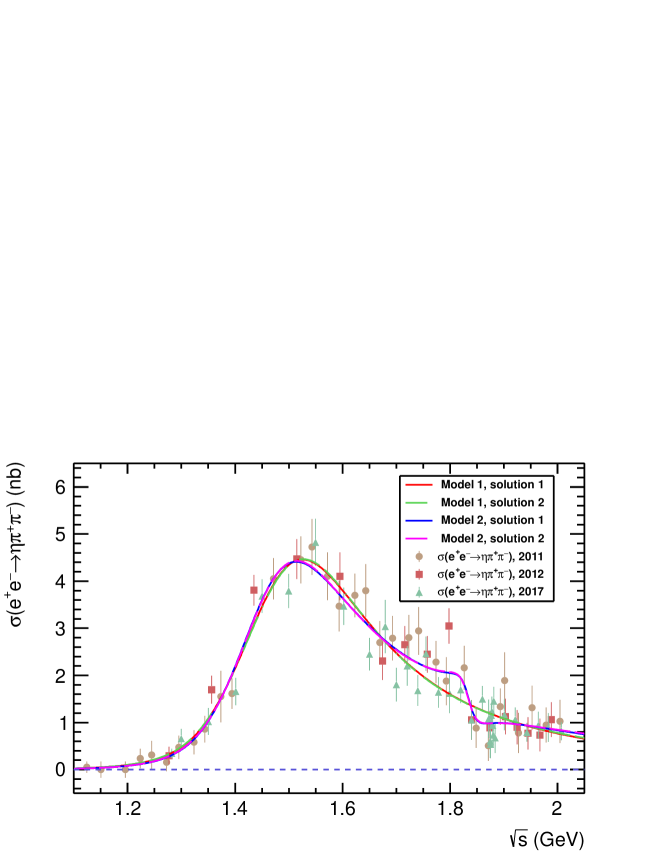
Figure 8: The $e^{+}e^{-}\rightarrow\eta\pi^{+}\pi^{-}$ Born cross section (points with error bars) measured with the CMD-3 detector and fitted with “Model 1, solution 1” (red solid curve), “Model 1, solution 2” (blue dashed curve), “Model 2, solution 1” (magenta solid curve) and “Model 2, solution 2” (green dashed curve). The “Model 1, solution 1” and “Model 1, solution 2” include contributions of $\rho(770)$ and $\rho(1450)$ and correspond to two different local minima of the fit chi-square. The“Model 2, solution 1” and “Model 2, solution 2” include contributions of $\rho(770)$, $\rho(1450)$ and $\rho(1700)$ and correspond to two different local minima of the fit chi-square.

Using parameters $\Gamma(\rho(1450)\rightarrow e^{+}e^{-})\mathcal{B}(\rho(1450)\rightarrow\eta\pi^{+}\pi^{-})$ and $\Gamma(\rho(1700)\rightarrow e^{+}e^{-})\mathcal{B}(\rho(1700)\rightarrow\eta\pi^{+}\pi^{-})$ instead of parameters $g_{\rho(1450)}$ and $g_{\rho(1700)}$ and the relation

$$\Gamma(V^{\prime}\rightarrow e^{+}e^{-})\mathcal{B}(V^{\prime}\rightarrow\eta\pi^{+}\pi^{-})=\frac{\alpha^{2}}{9\pi}\frac{|g_{V^{\prime}}|^{2}m_{V^{\prime}}}{\Gamma_{V^{\prime}}}\mathcal{I}(m^{2}_{V^{\prime}}),$$ (32)

we perform fits corresponding to solutions $1$–$2$ in each of the two models. The integral $\mathcal{I}$ has been defined in Eq. (18), $V^{\prime}$ is $\rho(1450)$ or $\rho(1700)$, $\Gamma_{V^{\prime}}$ is width of $V^{\prime}$ at $V^{\prime}$ mass, $m_{V^{\prime}}$. The fit results for the $\Gamma(\rho(1450)\rightarrow e^{+}e^{-})\mathcal{B}(\rho(1450)\rightarrow\eta\pi^{+}\pi^{-})$ and $\Gamma(\rho(1700)\rightarrow e^{+}e^{-})\mathcal{B}(\rho(1700)\rightarrow\eta\pi^{+}\pi^{-})$ products are presented in Table 5 and Table 6, respectively.

Table 5: The $\Gamma(\rho(1450)\rightarrow e^{+}e^{-})\mathcal{B}(\rho(1450)\rightarrow\eta\pi^{+}\pi^{-})$ products obtained from different fits, which correspond to solutions $1$–$2$ in each of the two models. The first uncertainty in each product is statistical, the last one is systematic.

Solution	$\Gamma(\rho(1450)\rightarrow e^{+}e^{-})\mathcal{B}(\rho(1450)\rightarrow\eta\pi^{+}\pi^{-})$, eV

Table 6: The $\Gamma(\rho(1700)\rightarrow e^{+}e^{-})\mathcal{B}(\rho(1700)\rightarrow\eta\pi^{+}\pi^{-})$ obtained from the different fits, which correspond to solutions $1$–$2$ of the second model. The first uncertainty in each product is statistical, the last one is systematic.

Solution	$\Gamma(\rho(1700)\rightarrow e^{+}e^{-})\mathcal{B}(\rho(1700)\rightarrow\eta\pi^{+}\pi^{-})$, eV

The $e^{+}e^{-}\rightarrow\eta\pi^{+}\pi^{-}$ Born cross section can be used to calculate the $\tau^{-}\rightarrow\eta\pi^{-}\pi^{0}\nu_{\tau}$ branching fraction. To reach this goal one has to use the following formula, which has been obtained under the CVC hypothesis [26]:

$$\frac{\mathcal{B}(\tau^{-}\rightarrow\eta\pi^{-}\pi^{0}\nu_{\tau})}{\mathcal{B}(\tau^{-}\rightarrow\nu_{\tau}e^{-}\bar{\nu_{e}})}=\frac{3\cos^{2}\theta_{C}}{2\pi\alpha^{2}m^{8}_{\tau}}\int\limits^{m^{2}_{\tau}}_{0}dq^{2}q^{2}\big{(}m^{2}_{\tau}-q^{2}\big{)}^{2}\big{(}m^{2}_{\tau}+2q^{2}\big{)}\sigma_{e^{+}e^{-}\rightarrow\eta\pi^{+}\pi^{-}}(q^{2}).$$ (33)

The calculation of the $\tau^{-}\rightarrow\eta\pi^{-}\pi^{0}\nu_{\tau}$ branching fraction using the CMD-3 data leads to the following result:

$$\mathcal{B}(\tau^{-}\rightarrow\eta\pi^{-}\pi^{0}\nu_{\tau})=(0.168\pm 0.006\pm 0.011)\%,$$ (34)

where the first uncertainty is statistical and the second is systematic. This result can be compared with the world average value $\big{(}0.139\pm 0.01\big{)}\%$ [43], the BaBar result $\big{(}0.163\pm 0.008\big{)}\%$ [37], the SND result $\big{(}0.156\pm 0.004\pm 0.010\big{)}\%$ [17] and with the CVC result $\big{(}0.153\pm 0.018\big{)}\%$ based on the earlier $e^{+}e^{-}\rightarrow\eta\pi^{+}\pi^{-}$ data [19].

IX Summary

The $e^{+}e^{-}\rightarrow\eta\pi^{+}\pi^{-}$ cross section has been measured with the CMD-3 detector in the c.m. energy range $1.2$–$2.0$ GeV using the $\eta$ decay mode $\eta\rightarrow\gamma\gamma$. The obtained result confirms previous $e^{+}e^{-}\rightarrow\eta\pi^{+}\pi^{-}$ cross section measurements.

The internal structure of the $\eta\pi^{+}\pi^{-}$ final state has been studied. It has been confirmed that the $\eta\rho(770)$ intermediate state is dominant.

The fit of the $e^{+}e^{-}\rightarrow\eta\pi^{+}\pi^{-}$ cross section data has been performed within the two models. One of them includes contributions of the $\rho(770)\rightarrow\rho(770)\eta$ and $\rho(1450)\rightarrow\rho(770)\eta$ intermediate mechanisms while the other one includes also a contribution of the $\rho(1700)\rightarrow\rho(770)\eta$. It has been found that there are a few local minima of the fit to the cross section depending on the choice of initial fit parameters.

The products $\Gamma(\rho(1450)\rightarrow e^{+}e^{-})\mathcal{B}(\rho(1450)\rightarrow\eta\pi^{+}\pi^{-})$ and $\Gamma(\rho(1700)\rightarrow e^{+}e^{-})\mathcal{B}(\rho(1700)\rightarrow\eta\pi^{+}\pi^{-})$ corresponding to each model and fit local minima were also found. The results for these products are listed in Tables 5, 6. The fits to the $e^{+}e^{-}\rightarrow\eta\pi^{+}\pi^{-}$ cross section data have been also used to calculate the $\tau^{-}\rightarrow\eta\pi^{-}\pi^{0}\nu_{\tau}$ branching fraction under the CVC hypothesis. The $\tau^{-}\rightarrow\eta\pi^{-}\pi^{0}\nu_{\tau}$ branching fraction predicted using the $e^{+}e^{-}\rightarrow\eta\pi^{+}\pi^{-}$ cross section data obtained with the CMD-3 detector agrees with the similar SND and BaBar predictions, and differs by $1.8$ standard deviations of the combined error from the world average value.

X Acknowledgments

The authors are grateful to the VEPP-2000 team for excellent machine operation. The work has been partially supported by the Russian Foundation for Basic Research grant No. 18-32-01020. Part of the work related to the multihadronic generator is supported by the grant of Ministry of Science and Higher Education No. 14.W03.31.0026.

References

- [1] E. V. Abakumova et al. Phys. Rev. Lett., 110:14042, 2013.
- [2] E. V. Abakumova et al. JINST, 10:T09001, 2015.
- [3] M. N. Achasov et al. Phys. Rev. D, 68:052006, 2003.
- [4] M. N. Achasov et al. JETP Lett., 92:80, 2010.
- [5] M. N. Achasov et al. Phys. Rev. D, 97:012008, 2018.
- [6] N. N. Achasov and V. A. Karnakov. JETP Lett., 39:285, 1984.
- [7] N. N. Achasov and A. A. Kozhevnikov. Phys. Rev. D, 55:2663, 1997.
- [8] S. Actis et al. Eur. Phys. J. C, 66:585, 2010.
- [9] S. Agostinelli et al. Nucl. Instr. Meth. A, 506:250, 2003.
- [10] R. R. Akhmetshin et al. Phys. Lett. B, 489:125, 2000.
- [11] R. R. Akhmetshin et al. JINST, 12:C07044, 2017.
- [12] R. R. Akhmetshin et al. JINST, 12:C08010, 2017.
- [13] R. R. Akhmetshin et al. Phys. Lett. B, 773:150, 2017.
- [14] A. V. Anisenkov et al. JINST, 12:P04011, 2017.
- [15] A. Antonelli et al. Phys. Lett. B, 212:133, 1988.
- [16] B. Aubert et al. Phys. Rev. D, 76:092005, 2007.
- [17] V. M. Aulchenko et al. Phys. Rev. D, 91:052013, March 2015.
- [18] D. Berkaev et al. Nucl. Phys. Proc. Suppl., 225-227:303–308, 2008.
- [19] V. Cherepanov and S. Eidelman. Nucl. Phys. Proc. Suppl., 218:231, 2011.
- [20] H. Czyż et al., editors. Mini-Proceedings, 14th meeting of the Working Group on Rad. Corrections and MC Generators for Low Energies, 2013.
- [21] V. V. Danilov et al., editors. Proceedings EPAC96, Barcelona, 1996.
- [22] N. Davidson, T. Przedzinski, and Z. Was. arXiv:1011.0937 [hep-ph], 2010.
- [23] M. Davier, A. Hoecker, B. Malaescu, and Z. Zhang. Eur. Phys. J. C, 77:827, 2017.
- [24] V. P. Druzhinin et al. Phys. Lett. B, 174:115, 1986.
- [25] S. I. Eidelman and V. N. Ivanchenko. Phys. Lett. B, 257:437–440, January 1991.
- [26] F. J. Gilman. Phys. Rev. D, 35:3541, 1987.
- [27] P. Golonka and Z. Was. Eur. Phys. J., C50:53–62, 2007.
- [28] F. Grancagnolo et al. Nucl. Instr. Meth. A, 623:114, 2010.
- [29] S.S. Gribanov. Inverse error matrix for the cross section. https://cmd.inp.nsk.su/~sgribanov/etapipi/etapipi-2gamma-inverse-error-matrix.txt.
- [30] M. Jamin, A. Pich, and J. Portoles. Phys. Lett. B, 640:176, 2006.
- [31] F. Jegerlehner. Acta Phys. Polon. B, 49:1157, 2018.
- [32] A. Keshavarzi, D. Nomura, and T. Teubner. Phys. Rev. D, 97:114025, 2018.
- [33] B. I. Khazin et al. Nucl. Phys. Proc. Suppl., 181–182:376–380, September 2008.
- [34] I. A. Koop et al. Nucl. Phys. Proc. Suppl., 181-182:371, 2008.
- [35] E. A. Kozyrev et al. Phys. Lett. B, 760:314–319, 2017.
- [36] E. A. Kuraev and V. S. Fadin. Sov. J. Nucl. Phys., 41:466, 1985.
- [37] J. P. Lees et al. Phys. Rev. D, 97:052007, 2018.
- [38] J. P. Lees et al. Phys. Rev. D, 98:112015, 2018.
- [39] V .M. Malyshev. arXiv:1505.01509 [physics.data-an], 2015.
- [40] A. E. Ryzhenenkov et al. JINST, 12:C07040, 2017.
- [41] P. Yu. Shatunov et al. Phys. Part. Nucl. Lett., 13:995, 2016.
- [42] D. Shwartz et al., editors. PoS ICHEP2016, 2016.
- [43] M. Tanabashi et al. Phys. Rev. D, 98:030001, 2018.