Fermionic dark matter via UV and IR freeze-in and its possible X-ray signature

Abstract

Non-observation of any dark matter signature at various direct detection experiments over the last decade keeps indicating that immensely popular WIMP paradigm may not be the actual theory of particle dark matter. Non-thermal dark matter produced through freeze-in is an attractive proposal, naturally explaining null results by virtue of its feeble couplings with the Standard Model (SM) particles. We consider a minimal extension of the SM by two gauge singlet fields namely, a $\mathbb{Z}_{2}$-odd fermion $\chi$ and a pseudo scalar $\tilde{\phi}$, where the former has interactions with the SM particles only at dimension five level and beyond. This introduces natural suppression in the interactions of $\chi$ by a heavy new physics scale $\Lambda$ and forces $\chi$ to be a non-thermal dark matter candidate.  We have studied the production of $\chi$ in detail taking into account both ultra-violate (UV), infra-red (IR) as well as mixed UV-IR freeze-in and found that for $10^{10}\,{\rm GeV}\,\leq\,\Lambda\leq 10^{15}$ GeV, $\chi$ is dominantly produced via UV and mixed UV-IR freeze-in when reheat temperature $T_{\rm RH}\gtrsim 10^{4}$ GeV and below which the production is dominated by IR and mixed freeze-in. Furthermore, we have considered the cascade annihilation$\chi\bar{\chi}\rightarrow\tilde{\phi}\tilde{\phi}\rightarrow 4\gamma$ to address the longstanding $\sim 3.5$ keV X-ray line observed from various galaxies and galaxy clusters. We have found that the long-lived intermediate state $\tilde{\phi}$ modifies dark matter density around the galactic centre to an effective density $\rho_{\rm eff}$ which strongly depends on the decay length of $\tilde{\phi}$. Finally, the allowed parameter space in $\Lambda-g$ plane ($g$ is the coupling between $\chi\bar{\chi}$ and $\tilde{\phi}$) is obtained by comparing our result with the XMM Newton observed X-ray flux from the centre of Milky Way galaxy in $2\sigma$ range.

I Introduction

The indirect evidence including flat galaxy rotation curve, bullet cluster observation, gravitational lensing of distant objects etc.  have firmly established the fact that in addition to the visible baryonic matter, our Universe is made of some mysterious non-baryonic, non-luminous matter which is commonly known as the dark matter (DM). Besides these indirect evidences, cosmic microwave background (CMB) anisotropy probing experiments like WMAP Hinshaw:2012aka and Planck Aghanim:2018eyx have measured the amount of dark matter present in the Universe based on $\Lambda$CDM model and the present value of dark matter relic density is $\Omega_{\rm DM}\,h^{2}=0.120\pm 0.001$. In spite of all these, the particle nature of DM and its production mechanism are not known to us to date. There exists a plethora of proposals in the literature for a viable dark matter candidate. Among them thermally generated cold dark matter is the most studied scenario. This type of dark matter candidates are classified as weakly interacting massive particle (WIMP) Roszkowski:2017nbc . The WIMP scenario naturally predicts a “cold” dark matter candidate having mass in the GeV to TeV range with a weak scale total annihilation cross section $\langle{\sigma{\rm v}\rangle}\simeq 3\times 10^{-26}$ cm³/s. In addition, this attractive scenario also predicts substantial scattering cross section with first generation of quarks (unless they are prohibited by some exotic symmetry of a particular model) and hence with nucleons as well, which can easily be measured by the present dark matter direct detection experiments. However, as of now no signature of dark matter has been observed at direct detection experiments resulting in severe exclusions of both spin independent ($\sigma_{\rm SI}$) and spin dependent ($\sigma_{\rm SD}$) scattering cross sections. In particular, $\sigma_{\rm SI}$ has the maximum exclusion of $4.1\times 10^{-47}$ cm² for $m_{DM}=30$ GeV by the XENON1T experiment Aprile:2018dbl . In future, experiments like XENONnT Aprile:2015uzo , LUX-ZEPLIN (LZ) Akerib:2018lyp and DARWIN Aalbers:2016jon will be sensitive enough to explore all the remaining parameter space above the neutrino floor, a region dominated by coherent elastic neutrino-nucleus scattering (CE${\nu}$NS), beyond which it is an extremely difficult task to identify a dark matter signal from the neutrino background Boehm:2018sux .

The null results of direct detection experiments raised a fundamental question about the scale of interaction of dark matter with baryons. As a result, there are many interesting proposals which predict diminutive interactions between visible and dark sectors and at the same time attain correct relic density as reported by the CMB experiment Planck. Non-thermal origin of dark matter is one of such frameworks where dark matter possesses extremely feeble interaction with other particles in the thermal bath. In this framework, it is assumed that the initial abundance of dark matter is almost negligible compared to other particles maintaining thermal equilibrium among themselves. This may be visualised in a situation where after the inflation, inflaton field predominantly decays into the visible sector particles rather than its dark sector counterparts. Here, dark matter particles are produced gradually from the decay as well as scattering of bath particles. This is known as the Freeze-in mechanism Hall:2009bx . Moreover, there are two types of freeze-in depending on the time of maximum production of dark matter. One of them is the ultra-violet (UV) freeze-in Hall:2009bx ; Elahi:2014fsa ; McDonald:2015ljz ; Chen:2017kvz where dark and visible sectors are connected by the higher dimensional operators only. As a result, abundance of dark matter becomes extremely sensitive to the initial history such as the reheat temperature ($T_{\rm RH}$) of the Universe. In this situation production of dark matter occurs only through scatterings. On the other hand, renormalisable interaction between dark and visible sectors leads to another kind of dark matter production which is dominated at around the temperature $T\sim$ mass of the initial state particles, when latter are in thermal equilibrium. Beyond this, as the temperature of the Universe drops below the mass of the mother particle, its number density becomes Boltzmann suppressed and the corresponding production mode of dark matter ceases. Unlike the previous case, this kind of freeze-in is mostly effective at the lowest possible temperature for a particular production process (i.e. either decay or scattering or both) hence this is known as the infrared (IR) freeze-in Hall:2009bx ; Yaguna:2011qn ; Blennow:2013jba ; Biswas:2015sva ; Co:2015pka ; Shakya:2015xnx ; Biswas:2016bfo ; Konig:2016dzg ; Biswas:2016yjr ; Bernal:2017kxu ; Biswas:2017tce ; Pandey:2017quk ; Biswas:2018aib ; Borah:2018gjk . Moreover, freeze-in can also be possible when initial state particles themselves remain out of thermal equilibrium and in such cases one needs to calculate first the distribution function of mother particle which later enters into the Boltzmann equation of dark matter Biswas:2016iyh ; Konig:2016dzg and in such cases the dark matter production era through freeze-in depends on the nature of distribution function of mother particle. In this work, we have studied both the UV freeze-in and IR freeze-in in a single framework and we also discuss a possible signature of our dark matter candidate via $\sim 3.5$ keV X-ray line. For that, we have extended the SM by adding a gauge singlet and $\mathbb{Z}_{2}$-odd Dirac fermion ($\chi$) and a gauge singlet pseudo scalar ($\tilde{\phi}$). The Dirac fermion $\chi$ is absolutely stable due to the unbroken $\mathbb{Z}_{2}$ symmetry and hence it is our dark matter candidate. Both the SM gauge invariance and also the invariance of $\mathbb{Z}_{2}$ symmetry dictate that $\chi$ does not have any direct interactions with the SM fields except that with the Higgs doublet $\Phi$ and that too is possible only using the gauge invariant operators having dimensions five (minimum) or more. As a result, the production of dark matter via UV freeze-in is possible before the electroweak symmetry breaking (EWSB) where pairs of $\chi$ and $\bar{\chi}$ are produced from scatterings of the components of $\Phi$ and also from the electroweak gauge bosons and gluons as well as top quark (involving a $\tilde{\phi}$ mediator). Moreover, the same operator between $\chi$ and $\Phi$ is also responsible for the late time production of dark matter via IR freeze-in, as after EWSB $\Phi$ gets a nonzero vacuum expectation value (VEV) and the dimension five operator decomposes into a four dimensional interaction term between the SM Higgs boson $h$ and $\chi\bar{\chi}$. In the IR freeze-in regime, in addition to the annihilations of $h\,h$, $g\,g$, $W^{+}W^{-}$, $Z\,Z$, and $\gamma\,\gamma$, pair annihilations of the SM fermions, pseudo scalar ($\tilde{\phi}$) and the decays of the SM Higgs boson $h$ and $\tilde{\phi}$ are the possible sources of $\chi\bar{\chi}$ production. However, we will see that $\tilde{\phi}$ with a mass larger than 163 eV cannot be produced thermally at the early Universe via Primakoff processes as it will overclose the Universe.  This can be evaded if the freeze-out temperature of $\tilde{\phi}$ production processes is larger than the reheat temperature of the Universe. In spite of this, in the present model $\tilde{\phi}$ can also be produced non-thermally from processes involving top quark in the initial state as well as from the decay of the SM Higgs boson ($h$) if $m_{\tilde{\phi}}\leq m_{h}/2$. Non-thermal production of $\tilde{\phi}$ from UV processes and its subsequent decay into $\chi\bar{\chi}$ via a dimesion four operator is dubbed as mixed UV-IR freeze-in scenario of $\chi$. In addition, depending on its mass and lifetime (varies mainly with $\Lambda$, $m_{\tilde{\phi}}$ and $\tilde{\phi}\chi\bar{\chi}$ coupling $g$) the pseudo scalar $\tilde{\phi}$ may also act as a decaying dark matter component. After solving the Boltzmann equation of $\chi$ considering all possible production processes in the collision term we have shown the allowed parameter space in $\Lambda-T_{\rm RH}$ plane, which satisfies dark matter relic density in $1\sigma$ range, where $\Lambda$ is the possible new physics scale. We have found that in the lower end of $\Lambda-T_{\rm RH}$ plane, contributions to the relic density come mainly from IR as well as mixed freeze-in whereas UV and mixed freeze-in contribute to the relic density for higher values of $T_{\rm RH}$ and $\Lambda$.

Finally, we have discussed an indirect signature of our dark matter candidate in detail. For that we have considered $\sim 3.5$ keV X-ray line emission from different galaxies and galaxy clusters. The observation of $\sim 3.5$ keV X-ray line by the XMM Newton X-ray observatory from various galaxy clusters including Perseus, Coma, Centaurus etc. was first reported in Bulbul:2014sua . Afterwards, there are studies by various groups claiming the presence of this line in the X-ray spectrum from the Andromeda galaxy Boyarsky:2014jta and also from the centre of our Milky Way galaxy Boyarsky:2014ska ; Jeltema:2014qfa . Furthermore, the Suzaku X-ray observatory has searched for the signature of the $3.5$ keV line in the four X-ray brightest galaxy clusters namely Perseus, Virgo, Coma and Ophiuchus and they have detected signal in the Perseus galaxy cluster only Urban:2014yda . More recently, the evidence of this X-ray line has also been found in the cosmic X-ray background by the Chandra X-ray Observatory Cappelluti:2017ywp . There are plenty of studies focusing on the explanation of this mysterious X-ray signal from dark matter decay in a wide class of beyond Standard Model (BSM) scenarios 1402.7335 ; 1403.0865 ; 1403.1536 ; 1403.1782 ; Kolda:2014ppa ; 1403.6503 ; 1403.6621 ; 1404.2220 ; 1404.3676 ; 1405.6967 ; 1412.4253 ; Arcadi:2014dca ; Biswas:2015sva ; 1503.06130 ; Biswas:2015bca ; 1604.01929 ; 1612.08621 ; Biswas:2017ait ; Bae:2017dpt . On the other hand, although in less numbers, there exist proposals involving dark matter annihilation as well Dudas:2014ixa ; Baek:2014poa ; Brdar:2017wgy . Nevertheless, the astrophysical explanation of this X-ray line in the form of atomic transitions in helium-like potassium and chlorine Phillips:2015wla ; Iakubovskyi:2015kwa , is also possible.  In this work, our explanation using annihilating dark matter is distinctly different from the earlier attempts. Here, our dark matter candidate $\chi$ undergoes a cascade annihilation in which first a pair of $\chi\bar{\chi}$ annihilates into $\tilde{\phi}\tilde{\phi}$ and thereafter each $\tilde{\phi}$ decays into two $\gamma$s. This type of dark matter annihilation produces a “box” shaped photon spectrum Ibarra:2012dw which gets a line shape as $m_{\chi}\rightarrow m_{\tilde{\phi}}$. In this scenario, we have derived necessary analytical expressions of the photon flux and have compared our result with the observed X-ray flux by XMM Newton from the centre of Milky Way galaxy Boyarsky:2014ska and finally have presented the allowed parameter space in the $\Lambda-g$ plane.

Rest of the article is organised as follows. In Section II we describe our model briefly. Detailed analysis of dark matter production via both UV and IR freeze-in has been presented in Section III. Possibility of $\tilde{\phi}$ as a decaying dark matter candidate is discussed in Section IV. The Section V deals with a comprehensive study of an indirect signature of our proposed dark matter candidate $\chi$ in the form of long-standing $\sim 3.5$ keV X-ray line. Finally, we summarise in Section VI.

II Model

In this section we will describe our model briefly. As we have mentioned in the previous section, we consider a minimal extension of the SM, where one can have both types of freeze-in (UV and IR) effects in the relic density of dark matter. For that we have extended the fermionic sector as well as the scalar sector of the SM by adding a Dirac fermion $\chi$ and a pseudo scalar $\tilde{\phi}$. Both $\chi$ and $\tilde{\phi}$ are singlet under the SM gauge group ${\rm SU}(3)_{c}\otimes{\rm SU}(2)_{L}\otimes{\rm U}(1)_{Y}$. Additionally, we have imposed a $\mathbb{Z}_{2}$ symmetry in the Lagrangian and we demand that only $\chi$ is odd under $\mathbb{Z}_{2}$. Due to this, the Dirac fermion $\chi$ cannot have any interaction with the SM fields up to the level of dimension four. The minimal operator describing interaction of $\chi$ with SM Higgs doublet $\Phi$ is a five dimensional operator suppressed by a mass scale $\Lambda$. However, $\chi$ has renormalisable interaction with the remaining non-standard particle $\tilde{\phi}$. On the other hand, being a pseudo scalar, the CP invariance restricts interactions of $\tilde{\phi}$ as well. Although unlike $\chi$, $\tilde{\phi}$ has interaction with the SM Higgs doublet at dimension four level, beyond that one can have interactions between $\tilde{\phi}$ and SM gauge bosons which have very rich phenomenology. Moreover, since $\tilde{\phi}$ does not have any VEV, there is no spontaneous CP-violation as well after symmetry breaking. In this scenario, Dirac fermion $\chi$ is our dark matter candidate which is absolutely stable due the unbroken $\mathbb{Z}_{2}$ symmetry. On the other hand, in some particular cases where the mass of $\tilde{\phi}$ is less than $m_{\chi}/2$, $\tilde{\phi}$ can be partially stable, contributing some fraction of total dark matter relic density at the present epoch and thus can act as a decaying dark matter candidate. Here the lifetime of $\tilde{\phi}$ is entirely controlled by the cut-off scale $\Lambda$.  The charges of all the fields under ${\rm SU}(3)_{c}\otimes{\rm SU}(2)_{L}\otimes{\rm U}(1)_{Y}$$\otimes\mathbb{Z}_{2}$ symmetry are listed in Table 1.

Field content	Charge under ${\rm SU}(3)_{c}\otimes{\rm SU}(2)_{L}\otimes{\rm U}(1)_{Y}$$\otimes\mathbb{Z}_{2}$ symmetry
$\ell_{L}=\begin{pmatrix}\nu_{e}\\ e\end{pmatrix}_{L},\,\begin{pmatrix}\nu_{\mu}\\ \mu\end{pmatrix}_{L},\,\begin{pmatrix}\nu_{\tau}\\ \tau\end{pmatrix}_{L}$	$(1,\,2,\,-1,\,+)$
$\ell_{R}=e_{R},\,\mu_{R},\,\tau_{R}$	$(1,\,1,\,-2,\,+)$
$Q_{L}$=$\begin{pmatrix}u\\ d\end{pmatrix}_{L},\,\begin{pmatrix}c\\ s\end{pmatrix}_{L},\,\begin{pmatrix}t\\ b\end{pmatrix}_{L}$	$(3,\,2,\,\frac{1}{3},\,+)$
$U_{R}=u_{R},\,c_{R},\,t_{R}$	$(1,\,1,\,\frac{4}{3},\,+)$
$D_{R}=d_{R},\,s_{R},\,b_{R}$	$(1,\,1,\,-\frac{2}{3},\,+)$
$\Phi=\begin{pmatrix}\phi^{+}\\ \phi^{0}\end{pmatrix}$	$(1,\,2,\,1,\,+)$
$\chi$	$(1,\,1,\,0,\,-)$
$\tilde{\phi}$	$(1,\,1,\,0,\,+)$

Table 1: Field content of our model and their charges under ${\rm SU}(3)_{c}\otimes{\rm SU}(2)_{L}\otimes{\rm U}(1)_{Y}$$\otimes\mathbb{Z}_{2}$.

The gauge invariant and CP conserving Lagrangian of our model is given by

$$\mathcal{L}= \mathcal{L}_{SM}+\overline{\chi}(i\,\not{\partial}-m_{\chi})\chi+\frac{1}{2}(\partial^{\mu}\tilde{\phi})(\partial_{\mu}\tilde{\phi})-\frac{1}{2}m_{\tilde{\phi}}\tilde{\phi}^{2}-\frac{\tilde{\phi}\,B_{\mu\nu}{\tilde{B}}^{{\mu\nu}}}{2\,\Lambda}-\frac{\tilde{\phi}\,W^{a}_{\mu\nu}{\tilde{W}_{a}}^{{\mu\nu}}}{2\,\Lambda}-\frac{\tilde{\phi}\,G^{b}_{\mu\nu}{\tilde{G}_{b}}^{{\mu\nu}}}{2\,\Lambda}$$ (1)

$$-\frac{y^{\ell}_{\alpha\,\beta}}{\Lambda}(i\,\overline{{\ell}_{L}}_{\alpha}\,\Phi\,\gamma_{5}\,{\ell_{R}}_{\beta}\,\tilde{\phi}+h.c)-\frac{y^{d}_{\alpha\,\beta}}{\Lambda}(i\,\overline{{Q_{L}}_{\alpha}}\,\Phi\,\gamma_{5}\,{D_{R}}_{\beta}\tilde{\phi}+h.c)-\frac{y^{u}_{\alpha\,\beta}}{\Lambda}(i\,\overline{{Q_{L}}_{\alpha}}\,\tilde{\Phi}\,\gamma_{5}\,{U_{R}}_{\beta}\tilde{\phi}+h.c)$$

$$-\frac{\overline{\chi}\chi\,\Phi^{\dagger}\Phi}{\Lambda}-g\,\overline{\chi}\gamma_{5}\chi\tilde{\phi}+\frac{\lambda}{2}\tilde{\phi}^{2}\Phi^{\dagger}\Phi\,,$$

where $\alpha,\,\beta$ are the generation indices, $\Lambda$ is some mass scale which represents the cut-off scale of our effective theory. $B_{\mu\nu}=\partial_{\mu}B_{\nu}-\partial_{\nu}B_{\mu}$ , $W^{a}_{\mu\nu}=\partial_{\mu}W^{a}_{\nu}-\partial_{\nu}W^{a}_{\mu}+i\,g_{2}\,\epsilon^{abc}\,W^{b}_{\mu}\,W^{c}_{\nu}$ ($a=1,\,2,\,3$) and $G^{b}_{\mu\nu}=\partial_{\mu}G^{b}_{\nu}-\partial_{\nu}G^{b}_{\mu}+i\,g_{3}\,f^{bcd}\,G^{c}_{\mu}\,G^{d}_{\nu}$ ($b=1\,...\,8$) are field strength tensors for U(1)_Y, SU(2)_L and SU(3)_c gauge groups while the corresponding gauge bosons are denoted by $B_{\mu}$, $W^{a}_{\mu}$ and $G^{b}_{\mu}$ respectively. Moreover, $g_{2}\,(g_{3})$ and $\epsilon^{abc}\,(f^{abc})$ are gauge couplings and structure constants of SU(2)_L (SU(3)_c) respectively. Further, in the above $\tilde{X}_{\mu\nu}$ ($X=B_{\mu}$, $W^{a}_{\mu}$, $G^{a}_{\mu}$) is the Hodge dual of field strength tensor and is defined as $\tilde{X}_{\mu\nu}=\frac{1}{2}\epsilon_{\mu\nu\rho\sigma}X^{\rho\sigma}$ with $\epsilon_{\mu\nu\rho\sigma}$ representing a four dimensional Levi-Civita symbol. Now, the combination between field strength tensor $X_{\mu\nu}$ and its Hodge dual tensor $\tilde{X}_{\mu\nu}$ gives a pseudo scalar which is invariant under the Lorentz transformation. Hence, a combination of this product with $\tilde{\phi}$ remains CP invariant.

In the above Lagrangian, we have added an extra $i\,(\equiv\sqrt{-1})$ in each interaction term between SM fermions and $\tilde{\phi}$ so that the fermionic bilinears and their hermitian conjugate form a pseudo scalar. Here, $\tilde{\Phi}$ is an SU(2)_L doublet with hypercharge -1 and is defined as $\tilde{\Phi}=i\,\sigma_{2}\Phi^{*}$, where $\sigma_{2}$ is the second Pauli spin matrix and all the fermionic fields have been defined in Table 1. Further, we would like to note here that the Yukawa couplings $y^{\ell}$, $y^{u}$ and $y^{d}$ are same as the Yukawa couplings associated with charged leptons, up-type quarks and down-type quarks in the SM respectively. This is required to avoid the flavour changing neutral current between the SM fermions and $\tilde{\phi}$. All these interaction terms between $\tilde{\phi}$ and the SM fields except Higgs boson are suppressed by the new physics scale $\Lambda$. Furthermore, as in the SM, here also electroweak symmetry is broken to residual U(1)_EM symmetry by the vacuum expectation value of the neutral component of doublet $\Phi$.

III Dark matter production via UV and IR freeze-in

In this work, our principal goal is to study both types of freeze-in mechanism in a single framework by minimally extending the SM. As we have already seen in the previous section, all the interactions of our dark matter candidate $\chi$ with the SM particles are suppressed by a heavy new physics scale $\Lambda$. This naturally ensures that our dark matter candidate $\chi$ has extremely feeble interactions with thermal bath containing SM particles. Consequently, $\chi$ always stays out of thermal equilibrium and behaves as a non-thermal relic. The genesis of non-thermal dark matter in the early Universe is known as the freeze-in mechanism Hall:2009bx and depending upon the nature of interaction of non-thermal dark matter candidate with other bath particles, there are two types of freeze-in namely UV freeze-in and IR freeze-in. In the present case, both types of freeze-in mechanisms are important for $\chi$ production at two different epochs. The UV freeze-in is possible due to the presence of higher dimensional interactions between $\chi$ and SM fermions, gauge bosons and in this process maximum $\chi$ production occurred when the temperature of the Universe was equal to $T_{\rm RH}$, the reheat temperature. On the other hand, after electroweak symmetry breaking (EWSB) additional $\chi$ particles are produced from the scatterings and decays of the SM particles via IR freeze-in mechanism. This is indeed possible because after SU(2)${}_{L}\otimes{\rm U}(1)_{Y}$ breaking, one can construct dimension three (responsible for both scattering and decay) as well as dimension four (responsible for scattering only) interactions involving $\chi$ and other SM particles from those higher dimensional operators. We have calculated both the UV and IR contributions to the relic density of our dark matter candidate $\chi$. The required interaction terms which are responsible for the UV contribution are given by,

$$\mathcal{L} \supset -\frac{\overline{\chi}\chi\Phi^{\dagger}\Phi}{\Lambda}-\frac{\epsilon^{\mu\nu\alpha\beta}\left(\partial_{\mu}B_{\nu}\right)\left(\partial_{\alpha}B_{\beta}\right)\tilde{\phi}}{\Lambda}-\frac{\epsilon^{\mu\nu\alpha\beta}\left(\partial_{\mu}W^{a}_{\nu}\right)\left(\partial_{\alpha}W^{a}_{\beta}\right)\tilde{\phi}}{\Lambda}-\frac{\epsilon^{\mu\nu\alpha\beta}\left(\partial_{\mu}G^{b}_{\nu}\right)\left(\partial_{\alpha}G^{b}_{\beta}\right)\tilde{\phi}}{\Lambda}\,$$ (2)

$$-\dfrac{i}{\Lambda}\sum_{i=1}^{3}\Bigg{\{}\sum_{\alpha=u,d}{y^{\alpha}_{ii}}\,\overline{q_{i}}_{L}\,\gamma_{5}\,{q_{i}}_{R}\,{\phi^{0}}^{*}\,+{y^{\ell}_{ii}}\,\overline{\ell_{i}}_{L}\,\gamma_{5}\,{\ell_{i}}_{R}\,{\phi^{0}}^{*}\,+h.c.\Bigg{\}}\tilde{\phi}\,-g\,\bar{\chi}\gamma_{5}\chi\,\tilde{\phi}\,.$$

Note that the Yukawa couplings will provide significant contribution only for the top quark. Since UV freeze-in occurs well above the electroweak symmetry breaking, at that time there is no mixing between hypercharge gauge boson $B_{\mu}$ and $W^{3}_{\mu}$. Therefore, during UV freeze-in $B_{\mu}$, $W_{\mu}^{a}$ ($a=1,\,2,\,3$) and $G_{\mu}^{b}$ ($b=1\,....\,8$) are physical gauge bosons and $\chi$ is produced from their annihilations mediated by pseudo scalar $\tilde{\phi}$. Moreover, $\chi$ can also be produced from the annihilations of $T_{3}=\frac{1}{2}$ and $-\frac{1}{2}$ components of the Higgs doublet $\Phi$ respectively, where the former one is no longer a Goldstone boson before the EWSB. Furthermore, one can also have the following scattering processes $t\,\bar{t}\rightarrow\Phi\,\tilde{\phi}$, $t\,\Phi\rightarrow t\,\tilde{\phi}$ and $\bar{t}\,\Phi\rightarrow\bar{t}\,\tilde{\phi}$, which are dominant in the UV regime. $\tilde{\phi}$ production involving these scattering processes with subsequent $\tilde{\phi}\rightarrow\bar{\chi}\chi$ is termed as mixed UV-IR freeze-in scenario as mentioned earlier.

The Feynman diagrams for all these processes which are contributing significantly towards $\chi$ production via UV freeze-in are shown in Fig. 1 and gauge boson-pseudo scalar vertices are given in Appendix A.

Regime	DM Production channels
Before EWSB
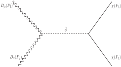
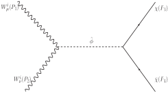
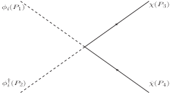
UV freeze-in of $\chi$

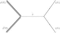
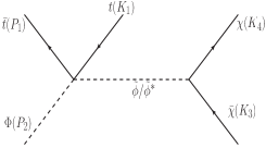
Figure 1: UV production channels of dark matter before EWSB.

On the other hand, IR freeze-in becomes effective only after the EWSB where we have three massive gauge bosons $W^{\pm}_{\mu}$, $Z_{\mu}$ and nine massless gauge boson $A_{\mu}$, $G_{\mu}^{a}$ as photon and gluons respectively in the particle spectrum. Additionally, our dark matter candidate can now have interactions with all the SM fermions and Higgs boson $h$. Depending on the mass of $\chi$, each of these particles have contributions to $\chi$ production in this regime. The interaction terms which govern IR production of $\chi$ are given by

$$\mathcal{L} \supset-\frac{\epsilon^{\mu\nu\alpha\beta}\left(\partial_{\mu}W^{-}_{\nu}\right)\left(\partial_{\alpha}W^{+}_{\beta}\right)\tilde{\phi}}{\Lambda}-\frac{\epsilon^{\mu\nu\alpha\beta}\left(\partial_{\mu}W^{+}_{\nu}\right)\left(\partial_{\alpha}W^{-}_{\beta}\right)\tilde{\phi}}{\Lambda}-\frac{\epsilon^{\mu\nu\alpha\beta}\left(\partial_{\mu}Z_{\nu}\right)\left(\partial_{\alpha}Z_{\beta}\right)\tilde{\phi}}{\Lambda}$$

$$-\frac{\epsilon^{\mu\nu\alpha\beta}(\partial_{\mu}A_{\nu})(\partial_{\alpha}A_{\beta})\tilde{\phi}}{\Lambda}-\frac{\epsilon^{\mu\nu\alpha\beta}\left(\partial_{\mu}G^{b}_{\nu}\right)\left(\partial_{\alpha}G^{b}_{\beta}\right)\tilde{\phi}}{\Lambda}-\dfrac{i}{\Lambda}\sum_{j}m_{f_{j}}\overline{f_{j}}\gamma_{5}f_{j}\tilde{\phi}$$

$$-\dfrac{\textit{v}}{\Lambda}\overline{\chi}\chi h-\frac{1}{2\Lambda}\overline{\chi}\chi\,h^{2}-g\,\overline{\chi}\gamma_{5}\chi\,\tilde{\phi}\,,$$ (3)

where $m_{f_{j}}$ is the mass of the SM fermion $f_{j}$ and the summation index $j$ is taken over all the SM fermions.

Therefore, our dark matter candidate $\chi$ has IR contributions to its relic density from the following scattering processes: $gg\rightarrow\overline{\chi}\chi$, $W^{+}W^{-}\rightarrow\overline{\chi}\chi$, $ZZ\rightarrow\overline{\chi}\chi$, $\bar{f}_{j}f_{j}\rightarrow\overline{\chi}\chi$, $hh\rightarrow\overline{\chi}\chi$ and $\tilde{\phi}\tilde{\phi}\rightarrow\overline{\chi}\chi$. Apart from these scatterings, $\chi$ can also be produced from the decays of Higgs boson $h$ and pseudo scalar $\tilde{\phi}$ if such processes are kinematically allowed. Feynman diagrams for all these processes are shown in Fig. 2. Moreover, we would like to comment here that as in this work we are considering $m_{\tilde{\phi}}\leq 100$ GeV, this choice does not allow $\tilde{\phi}$ to be generated thermally. This will become clear in the next section where we have a detailed discussion on this topic.

Regime	DM Production channels
After EWSB
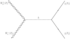
IR production of $\chi$

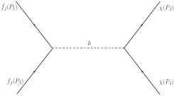
Figure 2: IR production channels of dark matter after EWSB.

Now, we calculate the relic abundance of $\chi$ produced via freeze-in. For that one needs to solve the Boltzmann equation of $\chi$, taking into account all possible interactions into the collision term. The Boltzmann equation of $\chi$ is given by

$$\frac{dn_{\chi}}{dt}+3Hn_{\chi} \simeq\sum_{i}n^{\rm eq}_{i}\,n^{\rm eq}_{i}\,\langle{\sigma\,{\rm v_{\rm rel}}\rangle_{i\,i\rightarrow\overline{\chi}\chi}}+n^{\rm eq}_{h}\,\langle{\Gamma_{h\rightarrow\overline{\chi}\chi}}\rangle$$

$$+\dfrac{g_{\tilde{\phi}}m_{\tilde{\phi}}\Gamma_{\tilde{\phi}\rightarrow\chi\bar{\chi}}}{2\pi^{2}}\int_{0}^{\infty}f(p,T)\dfrac{p^{2}dp}{\sqrt{p^{2}+m_{\tilde{\phi}}^{2}}}+\mathcal{F}_{2\rightarrow 3}(T)+\mathcal{F}_{2\rightarrow 4}(T)\,,$$ (4)

where, $n_{i}$ is the number density of species $i$ and the corresponding equilibrium number density is denoted by $n^{\rm eq}_{i}$. The second term in the left hand side of the Boltzmann equation proportional to the Hubble parameter $H$ dilutes $n_{\chi}$ due to the expansion of the Universe. In the right hand side, we have the usual collision term of the Boltzmann equation. Since we are dealing with a non-thermal dark matter candidate $\chi$ with an insignificant initial number density, in the collision term we have neglected backward reaction terms (inverse processes) proportional to $n^{2}_{\chi}$. Thus, in this case the collision term only contains all types of production processes of $\chi$ from annihilations as well as decays of other particles. The first term in the right hand side indicates the production of $\chi$ from scattering of particles $i$ which are in thermal equilibrium and their number densities only depend on mass of the corresponding particle and temperature of the Universe. The summation over $i$ is there to include all possible scattering processes. In principle, there can also be two different particles at the initial state of scattering, however, we are not considering such type of production processes of $\chi$ because those are not present in our present model. The scattering term has both UV and IR contributions. The epoch of UV production is determined by the reheat temperature $T_{\rm RH}$ of the Universe. However, for IR processes the production of dark matter from a particular decay(annihilation) becomes significant at around the temperature $T\sim m$, where $m$ being the mass of the initial state particle(s). Particularly, this is due to the reason that for temperature $T<<m$, the number density of mother particles following Maxwell-Boltzmann distribution gets exponentially suppressed.

The second part of the collision term represents the increase in number density of $\chi$ from decay of the SM Higgs ($h$). A detail derivation of the collision term for both scattering and decay processes are given in Appendices D and E.

The third part of the collision term indicates the production of $\chi$ via mixed freeze-in. Since $\tilde{\phi}$ is not in thermal equilibrium with the SM bath, the calculation of the abundance of $\chi$ from the decay of $\tilde{\phi}$, requires the knowledge of the momentum distribution function ($f(p,T)$) of $\tilde{\phi}$ . A detail derivation of momentum distribution function of $\tilde{\phi}$ is given in Appendix B. The fourth and fifth terms in Eq. (4) indicate the production of $\chi$ from $2\rightarrow 3$ and $2\rightarrow 4$ processes via off-shell $\tilde{\phi}$ and the detail calculation of these collision terms are given in Appendix C.

To solve the above equation, it is useful to consider a dimensionless variable namely the comoving number density of $\chi$, $Y_{\chi}=\dfrac{n_{\chi}}{s}$, which absorbs the effect of expansion of the Universe and indicates only the change in $n_{\chi}$ due to number changing processes involving dark matter candidate $\chi$ and other bath particles. Here the quantity $s$ is the entropy density of the Universe. Following the procedure as discussed in Appendices D and E for solution of the Boltzmann equation for both UV as well as IR freeze-in case, we now present the solution of the Boltzmann equation (value of $Y_{\chi}$ at the present epoch) as given below,

$$Y_{\chi}(T_{0}) \simeq 2\times\frac{1}{16\pi^{4}}\Bigg{[}\int_{T_{\rm EW}}^{T_{\rm RH}}\frac{dT}{sH}\,\int^{\infty}_{4\,m^{2}_{i}}d\hat{s}\,\sum_{i}\,\left(g_{i}^{2}\,\sigma_{ii\rightarrow\overline{\chi}\chi}\right)\,F\sqrt{\hat{s}-4\,m^{2}_{i}}\,{\rm K_{1}}\left(\frac{\sqrt{\hat{s}}}{T}\right)$$ (5)

$$+ 16\pi^{4}\left(\int_{T_{\rm EW}}^{T_{\rm RH}}\dfrac{dT}{sHT}\mathcal{F}_{2\rightarrow 3}(T)+\dfrac{g_{\tilde{\phi}}m_{\tilde{\phi}}\Gamma_{\tilde{\phi}\rightarrow\chi\bar{\chi}}}{2\pi^{2}}\int_{T_{0}}^{T_{\rm RH}}\dfrac{dT}{sHT}\int_{0}^{\infty}f(p,T)\dfrac{p^{2}dp}{\sqrt{p^{2}+m_{\tilde{\phi}}^{2}}}\right)$$

$$+ 16\pi^{4}\int_{T_{0}}^{T_{\rm EW}}\dfrac{dT}{sHT}\,\mathcal{F}_{2\rightarrow 4}(T)+\int_{T_{0}}^{T_{\rm EW}}\frac{dT}{sH}\,\int^{\infty}_{4\,m^{2}_{i}}d\hat{s}\,\sum_{i}\,\left(g_{i}^{2}\,\sigma_{ii\rightarrow\overline{\chi}\chi}\right)\,F\sqrt{\hat{s}-4\,m^{2}_{i}}\,{\rm K_{1}}\left(\frac{\sqrt{\hat{s}}}{T}\right)$$

$$+ 8\pi^{2}g_{h}\,m^{2}_{h}\,\Gamma_{h\rightarrow\overline{\chi}\chi}\int_{T_{0}}^{T_{\rm EW}}\dfrac{dT}{sH}{\rm K_{1}}\left(\frac{m_{h}}{T}\right)\Bigg{]}\,.$$

Here, the first two terms are the UV contribution to $Y_{\chi}$ and it is clearly visible that these parts depend on the reheat temperature $T_{\rm RH}$. The third term is the production of $\chi$ via mixed freeze-in which is present before and after EWSB. On the other hand, the next part is coming from the IR contributions to $Y_{\chi}$ and it becomes effective only after the EWSB. This is because after the EWSB, Higgs doublet gets a nonzero VEV and there are renormalisable interactions (up to a level of dimension four) between dark matter and Higgs. The last term is another IR contribution to $Y_{\chi}$ originating from the decay of $h$. In the above, $m_{i}$, $g_{i}$ are mass and internal degrees of freedom of particle $i$ while $T_{\rm EW}$ and $T_{0}$ are EWSB temperature and temperature at the present epoch. Moreover, as discussed in the Appendices D and E, one can further simplify UV contribution and IR contribution from $h$ decay. On the other hand, the decay $\tilde{\phi}\rightarrow\bar{\chi}\chi$, UV freeze-in terms originating from $2\rightarrow 3$ processes and IR freeze-in term originating from $2\rightarrow 4$ process require knowledge of $f(p,T)$, $\mathcal{F}_{2\rightarrow 3}$, $\mathcal{F}_{2\rightarrow 4}$ respectively, which are discussed in detail in Appendices B and C. Simplification of IR freeze-in term (fifth term in the right hand side of Eq.  (5)) originating from the scatterings requires knowledge about cross sections of all the production processes. Therefore, the solution of the Boltzmann equation after those simplifications can be written in a more compact form as follows

$$Y_{\chi}(T_{0}) \simeq 2\times\dfrac{M_{pl}}{1.66\,(2\pi)^{3}}\Bigg{[}\dfrac{180\,\left(16g^{2}+32g^{2}+4\right)}{(2\pi)^{4}\,\sqrt{g_{\rho}(T_{\rm RH})}\,g_{s}(T_{\rm RH})}\dfrac{T_{\rm RH}-T_{\rm EW}}{\Lambda^{2}}+135\left(\dfrac{g_{h}\,\Gamma_{h\rightarrow\overline{\chi}\chi}}{m^{2}_{h}\,\sqrt{g_{\rho}(m_{h})}\,g_{s}(m_{h})}\right)\Bigg{]}$$

$$+ 2\left(\int_{T_{\rm EW}}^{T_{\rm RH}}\dfrac{dT}{sHT}\mathcal{F}_{2\rightarrow 3}(T)+\dfrac{g_{\tilde{\phi}}m_{\tilde{\phi}}\Gamma_{\tilde{\phi}\rightarrow\chi\bar{\chi}}}{2\pi^{2}}\int_{T_{0}}^{T_{\rm RH}}\dfrac{dT}{sHT}\int_{0}^{\infty}f(p,T)\dfrac{p^{2}dp}{\sqrt{p^{2}+m_{\tilde{\phi}}^{2}}}\right)$$

$$+ 2\int_{T_{0}}^{T_{\rm EW}}\dfrac{dT}{sHT}\mathcal{F}_{2\rightarrow 4}(T)+\frac{1}{8\pi^{4}}\int_{T_{0}}^{T_{\rm EW}}\frac{dT}{sH}\,\int^{\infty}_{4\,m^{2}_{i}}d\hat{s}\,\sum_{i}\,\left(g_{i}^{2}\,\sigma_{ii\rightarrow\overline{\chi}\chi}\right)\,F\sqrt{\hat{s}-4\,m^{2}_{i}}\,{\rm K_{1}}\left(\frac{\sqrt{\hat{s}}}{T}\right)\,.$$

Here, the factor $\left(16g^{2}+32g^{2}+4\right)$ in the first term comes from fourteen scattering diagrams including four electroweak gauge boson annihilations, eight gluon annihilations and two scalar annihilations into $\overline{\chi}\chi$ pairs (see Feynman diagrams in Fig. 1). Below we have listed all the relevant scattering cross sections and decay widths which are required to find $Y_{\chi}$ at $T_{0}$ using Eq. (LABEL:ychiT0) and the corresponding Feynman diagrams are illustrated in Fig. 2.

$$\sigma_{ZZ\rightarrow\bar{\chi}\chi}= \frac{1}{16\pi\hat{s}}\sqrt{\frac{\hat{s}-4m_{\chi}^{2}}{\hat{s}-4m_{Z}^{2}}}\Bigg{[}\frac{8m_{Z}^{4}}{9\Lambda^{2}}\frac{(\hat{s}-4m_{\chi}^{2})(3+\frac{\hat{s}^{2}}{4m_{Z}^{4}}-\frac{\hat{s}}{m_{Z}^{2}})}{(\hat{s}-m_{h}^{2})^{2}}+\frac{4g^{2}}{9\Lambda^{2}}\frac{\hat{s}^{2}(\hat{s}-4m_{Z}^{2})}{(\hat{s}-m_{\tilde{\phi}}^{2})^{2}}\Bigg{]}\,,$$ (7a)

$$\sigma_{W^{+}W^{-}\rightarrow\bar{\chi}\chi}= \frac{1}{16\pi\hat{s}}\sqrt{\frac{\hat{s}-4m_{\chi}^{2}}{\hat{s}-4m_{W}^{2}}}\Bigg{[}\frac{8m_{W}^{4}}{9\Lambda^{2}}\frac{(\hat{s}-4m_{\chi}^{2})(3+\frac{\hat{s}^{2}}{4m_{W}^{4}}-\frac{\hat{s}}{m_{W}^{2}})}{(\hat{s}-m_{h}^{2})^{2}}+\frac{4g^{2}}{9\Lambda^{2}}\frac{\hat{s}^{2}(\hat{s}-4m_{W}^{2})}{(\hat{s}-m_{\tilde{\phi}}^{2})^{2}}\Bigg{]}\,,$$ (7b)

$$\sigma_{\gamma\gamma\rightarrow\bar{\chi}\chi}= \frac{g^{2}\hat{s}^{\frac{3}{2}}}{16\pi\Lambda^{2}}\frac{\sqrt{\hat{s}-4m_{\chi}^{2}}}{(\hat{s}-m_{\tilde{\phi}}^{2})^{2}}\,,$$ (7c)

$$\sigma_{\bar{f_{i}}f_{i}\rightarrow\bar{\chi}\chi}= \frac{1}{16\pi\hat{s}}\sqrt{\frac{\hat{s}-4m_{\chi}^{2}}{\hat{s}-4m_{f_{i}}^{2}}}\Bigg{[}\frac{m_{f_{i}}^{2}(\hat{s}-4m_{f_{i}}^{2})(\hat{s}-4m_{\chi}^{2})}{\Lambda^{2}(\hat{s}-m_{h}^{2})^{2}}+\frac{g^{2}\hat{s}^{2}\,m_{f_{i}}^{2}}{\Lambda^{2}(\hat{s}-m_{\tilde{\phi}^{2}})^{2}}\Bigg{]}\,,$$ (7d)

$$\sigma_{hh\rightarrow\bar{\chi}\chi}= \frac{1}{8\pi\hat{s}\Lambda^{2}}\Bigg{[}1+\frac{9m_{h}^{4}}{(\hat{s}-m_{h}^{2})^{2}}\Bigg{]}\frac{(\hat{s}-4m_{\chi}^{2})^{\frac{3}{2}}}{\sqrt{\hat{s}-4m_{h}^{2}}}\,,$$ (7e)

$$\sigma_{gg\rightarrow\bar{\chi}\chi}= \frac{1}{16\pi\Lambda^{2}}\left[\frac{g^{2}\hat{s}^{\frac{3}{2}}\sqrt{\hat{s}-4m_{\chi}^{2}}}{8(\hat{s}-m_{\tilde{\phi}}^{2})^{2}}\,+\frac{|c_{ggh}|^{2}v^{2}\sqrt{\hat{s}(\hat{s}-4m_{\chi}^{2})^{3}}}{8(\hat{s}-m_{h}^{2})^{2}}\right]\,,$$ (7f)

$$\Gamma_{h\rightarrow\bar{\chi}\chi}= \frac{\textit{v}^{2}}{\Lambda^{2}}\frac{m_{h}}{8\pi}\Bigg{(}1-\frac{4m_{\chi}^{2}}{m_{h}^{2}}\Bigg{)}^{\frac{3}{2}}\,,$$ (7g)

$$\Gamma_{\tilde{\phi}\rightarrow\bar{\chi}\chi}= \dfrac{g^{2}m_{\tilde{\phi}}}{8\pi}\sqrt{1-\dfrac{4m_{\chi}^{2}}{m_{\tilde{\phi}}^{2}}}\,.$$ (7h)

In Eq. (7f), $c_{ggh}$ is the loop factor of the process $gg\rightarrow\bar{\chi}\chi$ which is given by Barger:1987nn

$$c_{ggh}(\hat{s})=-(\sqrt{2}G_{F})^{\frac{1}{2}}\frac{\alpha_{s}(\hat{s})}{12\pi}\sum_{q}I_{q}\,,$$

and

$$I_{q}=3\int_{0}^{1}dx\int_{0}^{1-x}dy\,\dfrac{1-4xy}{1-\dfrac{xy}{\lambda_{q}}}\,,$$

where $\lambda_{q}=\frac{m_{q}^{2}}{\hat{s}}$. The loop integral $I_{q}$ has the following form

$$I_{q}=3\left[2\lambda_{q}+\lambda_{q}\left(4\lambda_{q}-1\right)f(\lambda_{q})\right]\,.$$

The function $f(\lambda_{q})$ is given by

$$f(\lambda_{q}) = -2\left(\arcsin\dfrac{1}{2\sqrt{\lambda_{q}}}\right)^{2}\,,\,\,\,\,\,\,\,\,\,\,\,\,\,\,\,\,\,\,\,\,\,\,\,\,\,\,\,\,\,\,\,\text{for}\,\lambda_{q}>\frac{1}{4}\,,$$

$$= \frac{1}{2}\left(\log\frac{\eta^{+}}{\eta^{-}}\right)^{2}-\frac{\pi^{2}}{2}-i\pi\log\frac{\eta^{+}}{\eta^{-}}\,,\,\,\,\,\,\,\,\,\text{for}\,\lambda_{q}<\frac{1}{4}\,,$$

with $\eta^{\pm}=\dfrac{1}{2}\pm\sqrt{\dfrac{1}{4}-\lambda_{q}}$   .

Finally, the relic density ($\Omega_{\chi}h^{2}$) of $\chi$ is defined as the ratio of dark matter mass density to the critical density ($\rho_{\rm crit}$) of the Universe and it is related to comoving number density ($Y_{\chi}(T_{0})$) by the following relation Gondolo:1990dk ; Edsjo:1997bg ,

$$\Omega_{\chi}h^{2}=2.755\times 10^{8}\dfrac{m_{\chi}}{\rm GeV}\,Y_{\chi}(T_{0})\,.$$ (8)

Let us note in passing that the dominant production channels of $\chi$ are $\phi_{i}^{\dagger}\phi_{i}\rightarrow\bar{\chi}\chi$ in the UV regime and $W^{+}W^{-}\rightarrow\bar{\chi}\chi$, $ZZ\rightarrow\bar{\chi}\chi$, $hh\rightarrow\bar{\chi}\chi$, $h\rightarrow\bar{\chi}\chi$ in IR regime. Mixed freeze-in can contribute to the relic density of $\chi$ in both UV and IR regime.

III.1 Numerical results of the Boltzmann Equation

In this section, we present the allowed parameter space that we have obtained by computing dark matter relic density using Eqs. (LABEL:ychiT0-8) and comparing this with the reported range of $\Omega_{\rm DM}h^{2}=0.120\pm 0.001$ by the Planck experiment. In order to do this, we have varied the independent parameters $\Lambda$, $T_{\rm RH}$, $m_{\chi}$, $g$ and $\lambda$ within the following ranges.

$$\begin{array}[]{cccccc}10^{10}\,\text{GeV}\leq&\Lambda&\leq 10^{15}\,\text{GeV}\,\,,\\ 10^{3}\,\text{GeV}\leq&T_{\rm RH}&\leq 10^{13}\,\text{GeV}\,\,,\\ 10^{-6}\,\text{GeV}\leq&m_{\chi}&\leq 10^{2}\,\text{GeV}\,\,,\\ 10^{-8}\leq&g&\leq 10^{-2}\,\,,\\ 10^{-12}\leq&\lambda&\leq 10^{-8}\,\,,\end{array}$$ (14)

The allowed parameter space in the $T_{\rm RH}-\Lambda$ plane by the relic density constraint is shown in the left panel of Fig. 3.

Figure 3: Left panel: The $T_{\rm RH}-\Lambda$ parameter space reproducing correct dark matter relic density via freeze-in mechanism for $m_{\tilde{\phi}}=100$ GeV and $1\,\text{keV}\leq m_{\chi}\leq 100$ GeV. Here cyan, red, green points indiacate fractional contribution of UV, IR and mixed freeze-in greater than 60 $\%$ respectively. The black points indicate that the fractional contributions both of UV and IR freeze-in less than 60$\%$. Right panel: Corresponding values of $T_{\rm RH}$ and $\Lambda$ for $m_{\tilde{\phi}}\simeq m_{\chi}=7.06$ keV. Colour codes are same as those in the left panel.

In the present work, as mentioned earlier, different types of freeze-in mechanisms are contributing to the relic density of our dark matter candidate $\chi$. From this figure it is clearly visible that UV freeze-in contributes maximally for large reheat temperature i.e. $T_{\rm RH}>10^{4}$ GeV. This can be understood easily from the first term of Eq. (LABEL:ychiT0), where we see that the UV effect on $Y_{\chi}(T_{0})$ is proportional to $T_{\rm RH}$. Moreover, the contribution of UV freeze-in to $Y_{\chi}(T_{0})$ has a $1/\Lambda^{2}$ suppression, as a result one needs larger $\Lambda$ for higher $T_{\rm RH}$ such that $\Omega_{\chi}h^{2}$ does not exceed $1\sigma$ allowed range of $\Omega_{\rm DM}h^{2}$. We already know that IR freeze-in can occur from both decay and scattering of the parent particles. For low reheat temperature ($T_{\rm RH}<10^{4}$ GeV), scatterings of $W$, $Z$, $h$ and decay of the Higgs boson are the dominant sources of IR freeze-in. An additional source of significant production of $\chi$ is via mixed freeze-in. As a result, $\tilde{\phi}$ production from the scatterings involving top quark and subsequent decay of $\tilde{\phi}$ into $\bar{\chi}\chi$ pair gives substantial contribution to $\Omega_{\chi}h^{2}$. Furthermore, the variation of $\Lambda$ for a particular value of $T_{\rm RH}$ is mostly due to $g$ and $m_{\chi}$ where the latter is varying between 1 keV to 100 GeV. The same parameter space for $m_{\tilde{\phi}}\simeq m_{\chi}=7.06$ keV is shown in the right panel of Fig. 3. Here we get UV freeze-in dominance for higher values of $T_{\rm RH}$ and $\Lambda$ whereas for low reheating temperature ($T_{\rm RH}<10^{4}$ GeV) IR freeze-in becomes superior. The absence of mixed freeze-in of $\chi$ is due to the fact that in this case the decay of $\tilde{\phi}$ to ${\chi}\bar{\chi}$ pair is kinematically forbidden. On top of that another noticeable difference is that instead of getting an allowed region in the $T_{\rm RH}-\Lambda$ plane here we get a line and this is mainly due to the reason that in the present plot we have kept $m_{\chi}$ fixed at $7.06$ keV.

IV Possibility of $\tilde{\phi}$ as one of the dark matter components

In this section, we discuss about the possibility of having $\tilde{\phi}$ as another dark matter component besides $\chi$. Since $\tilde{\phi}$ has interaction with photons, it can be produced thermally from the inelastic scattering between any charged fermions ($f$) and $\gamma$ at the early Universe. Such type of scatterings $f+\gamma\rightarrow f+\tilde{\phi}$ are known as the Primakoff process, where at the final state from each scattering a $\tilde{\phi}$ and a charged fermion are produced. Moreover, as we have interactions like $\bar{f}\gamma_{5}f\tilde{\phi}$ with $f$ being any SM fermion, the Primakoff scattering can also be possible here through an $s$-channel mediator $f$ after EWSB. However, extremely suppressed coupling (a ratio between the SM Yukawa coupling and the new physics scale $\Lambda$) of $\bar{f}f$ with $\tilde{\phi}$ makes such processes insignificant. On the other hand, in the present scenario, $\tilde{\phi}$ can also be produced from the Primakoff like processes where photons are replaced by other SM gauge bosons $Z$ and $W^{\pm}$. Therefore, following the procedure given in Cadamuro:2011fd , we have found that the freeze-out temperature $T_{f}$ of $\tilde{\phi}$ always remains larger than 100 GeV as long as $\Lambda\gtrsim 10^{9}$ GeV. This implies $\tilde{\phi}$ (of mass $m_{\tilde{\phi}}\lesssim 100$ GeV) freezes-out relativistically when $\Lambda\gtrsim 10^{9}$ GeV, which is the range of $\Lambda$ we are considering in this work and also is allowed from various astroparticle physics experiments Cadamuro:2011fd . As a result of this relativistic freeze-out, once we know the freeze-out temperature $T_{f}$, the number density of $\tilde{\phi}$ at the present epoch becomes fixed from the following relation as

$$n_{\tilde{\phi}}(T_{0})=\dfrac{n_{\gamma}(T_{0})}{2}\dfrac{g_{s}(T_{0})}{g_{s}(T_{f})}\,,$$ (15)

where $n_{\gamma}(T_{0})$ is the number density of $\gamma$ at the present epoch, $T_{0}=2.73$ K being the present average temperature of the Universe and $g_{s}(T)$ is the number of relativistic degrees of freedom present at temperature $T$ which are contributing to the entropy density of the Universe. Using $n_{\tilde{\phi}}$, now one can calculate the relic density of $\tilde{\phi}$ easily which is given by Kolb:1990vq

$$\Omega_{\tilde{\phi}}h^{2}=0.12\times\left(\dfrac{m_{\tilde{\phi}}}{163\,{\rm eV}}\right)\times\left(\dfrac{106.75}{g_{s}(T_{f})}\right)\,\,.$$ (16)

Therefore, $\tilde{\phi}$ with mass larger than 163  eV will overclose the Universe. In order to avoid this unpleasant situation, one needs the freeze-out temperature $T_{f}$ of $\tilde{\phi}$ to be larger than the reheat temperature ($T_{\rm RH}$) of the Universe such that $\tilde{\phi}$ will never be produced thermally from the Primakoff process. This condition is indeed satisfied in the present work since the allowed range of $T_{\rm RH}$ for a particular value of new physics scale $\Lambda$ (see Fig. 3 in Section III.1) always lies below the freeze-out temperature $T_{f}$ of the Primakoff process, which has the following approximate dependence on $\Lambda$ as $T_{f}\simeq 1.259\times 10^{-16}\,\Lambda^{2}$ Cadamuro:2011fd .

As discussed in Section III, in the present model, there are some additional sources of $\tilde{\phi}$ production via UV and IR freeze-in. However, $\tilde{\phi}$ will be produced dominantly via UV-freeze-in from the processes like $t\,\bar{t}\rightarrow\Phi\,\tilde{\phi}$, $t\,\Phi\rightarrow t\,\tilde{\phi}$ and $\bar{t}\,\Phi\rightarrow\bar{t}\,\tilde{\phi}$ where the abundance of $\tilde{\phi}$ depends on $T_{RH}$ and $\Lambda$. Assuming the mass of $\tilde{\phi}$ to be $\sim 7$ keV and $m_{\chi}\gtrsim m_{\tilde{\phi}}$ (the reason for such a choice will be discussed in the next section) $\tilde{\phi}$ has only $\gamma\,\gamma$ decay mode available. Therefore,the way to make $\tilde{\phi}$ partially stable is by increasing $\Lambda$. One can easily check from Eq. (58) that for $\Lambda\geq 10^{12}$ GeV, the lifetime of $\tilde{\phi}$ becomes larger than the present age of the Universe, which is $\sim 10^{17}$ s. In that case the contribution of $\tilde{\phi}$ to the total dark matter relic density will be comparable to that coming from $\chi$. In such a scenario the value of $\Lambda$ in the range between $10^{12}$ GeV and $10^{17}$ GeV is strongly disfavored from extragalactic background light (EBL) and X-ray observations 1402.7335 . Nevertheless, the new physics scale $\Lambda>10^{17}$ GeV is allowed for a keV scale $\tilde{\phi}$. However, for such a large value of $\Lambda$, the abundance of $\tilde{\phi}$ is inadequate to contribute significantly to the overall dark matter relic density as the UV production processes of $\tilde{\phi}$ are suppressed by $\Lambda^{-2}$. It may appear that such a large value of $\Lambda$ will also affect the abundance of our principal dark matter candidate $\chi$. One can easily avoid this by assigning two different scales of interactions associated with $\tilde{\phi}$ and $\chi$ respectively. In this case, the UV production of $\chi$ from the scatterings of the components of $\Phi$ will be sufficient enough to reproduce the observed dark matter relic density.

V Indirect signature of $\chi$ via ${\sim\mathbf{3.5}}$ keV X-ray line

In the present model, our dark matter candidate $\chi$ can annihilate into a pair of $\tilde{\phi}$, which further decays into $\gamma\gamma$ final state i.e. $\bar{\chi}{\chi}\rightarrow\tilde{\phi}\tilde{\phi}\rightarrow 4\gamma$. Such cascade annihilation of $\chi$ results in a box shaped diffuse $\gamma$-ray spectrum Ibarra:2012dw , with each emitted photon has energy $m_{\tilde{\phi}}/2$ in the rest frame of $\tilde{\phi}$. The photon energy $E_{\gamma}$ in the laboratory frame where dark matter particle $\chi$ is assumed to be non-relativistic (i.e.  each intermediate scalar ($\tilde{\phi}$) has energy equal to $m_{\chi}$) is

$$E_{\gamma}=\dfrac{m^{2}_{\tilde{\phi}}}{2\,m_{\chi}}\left(1-\cos\theta\,\sqrt{1-\dfrac{m^{2}_{\tilde{\phi}}}{m^{2}_{\chi}}}\right)^{-1}\,,$$ (17)

where $\theta$ is the angle between $\tilde{\phi}$ and $\gamma$ in the laboratory frame. The maximum and the minimum energies $E^{max}_{\gamma}$ and $E^{min}_{\gamma}$ of $\gamma$ are obtained by putting $\theta=0$ and $\theta=\pi$ in the above expression. Moreover, as the intermediate state is a scalar, we will always have an isotropic photon emission in the rest frame of the scalar and also with respect to the laboratory frame if the intermediate scalar is non-relativistic. Thus, the resulting spectrum remains constant in energy with two sharp cut-off at energies $E^{max}_{\gamma}$ and $E^{min}_{\gamma}$ respectively and mimics a “box-shaped” spectrum. The width of the spectrum is given by,

$$\Delta{E} = E^{max}_{\gamma}-E^{min}_{\gamma}\,,$$ (18)

$$= \sqrt{m^{2}_{\chi}-m^{2}_{\tilde{\phi}}}\,,$$

which depends on the mass splitting between dark matter $\chi$ and pseudo scalar $\tilde{\phi}$. Therefore, the box-shaped photon spectrum becomes line like if $\chi$ and $\tilde{\phi}$ are exactly degenerate in mass. However, in this case we will have four photons per $\chi$ annihilation with each having energy $m_{\chi}/2$, which is not the situation when a $\gamma$-ray line spectrum is obtained from a prompt annihilation of $\chi$ and $\bar{\chi}$. In the later case, one gets two photons each having energy $m_{\chi}$ from a single $\chi\bar{\chi}$ annihilation.

Now, we want to demonstrate that the cascade annihilation of $\chi$ into 4 $\gamma$ final state can explain the long-standing $\sim 3.5$ keV X-ray line initially observed by the XMM Newton observatory from various galaxy clusters including Perseus, Centaurus, Coma etc. and also from the centre of our Milky Way galaxy. The excess X-ray flux observed from centre of the Milky Way galaxy within an angle of $14^{\prime}$ is $\left(29\pm 5\right)\times 10^{-6}$ cts/sec/cm² at an energy $E_{\gamma}=3.539\pm 0.011$ keV Boyarsky:2014ska . Therefore, for the rest of this section we have considered $m_{\chi}=7.06$ keV and $\delta=(m_{\chi}-m_{\tilde{\phi}})/m_{\chi}\sim 10^{-5}$ to match with the observed line like X-ray spectrum. However, there are strong bounds on the coupling of a keV scale pseudo scalar $\tilde{\phi}$ with photons from various astrophysical and cosmological phenomena. These include bounds Cadamuro:2011fd ; Bauer:2017ris from the detection of EBL, distortion in the cosmic microwave background (CMB) spectrum, measurement of effective number of relativistic degrees of freedom ($N_{eff}$) at the time of CMB formation, alternation in the successful prediction of Helium and Deuterium abundances from Big-Bang-Nucleosynthesis (BBN), length measurement of the neutrino burst from the SN1987a Supernova, the energy loss of stars through radiation (Horizontal Branch stars) etc. The present upper bound on $\tilde{\phi}\gamma\gamma$ coupling, which is inversely proportional to $\Lambda$ in our case, from all the above mentioned observations is $C_{\tilde{\phi}\gamma\gamma}\lesssim 10^{-17}$ GeV for a keV scale pseudo scalar $\tilde{\phi}$ 1402.7335 ; Cadamuro:2011fd .

However, this bound has been derived by considering $\tilde{\phi}$ contributing $100\%$ to the dark matter relic density. Here as discussed in the previous section, a keV scale $\tilde{\phi}$ depending upon its two photon coupling $C_{\tilde{\phi}\gamma\gamma}$ can be stable over the cosmological time scale and its abundance at the present epoch will be determined by an interplay between the rate of production of $\tilde{\phi}$ and the rate of decay into $\gamma\gamma$. In our case, $\tilde{\phi}$ is mostly produced via UV-freeze in from annihilations and scatterings of top quarks and for $\Lambda\gtrsim 10^{12}$ GeV, the contributions of $\tilde{\phi}$ and $\chi$ are comparable in the relic density. In this scenario with $\Lambda$ ranging between $10^{12}$ GeV to $10^{17}$ GeV is disfavoured from EBL and X-ray observations. Thus, for $m_{\tilde{\phi}}\simeq m_{\chi}$ and $m_{\tilde{\phi}}\sim$ 7 keV, we have considered the mass scale $10^{10}$ GeV$\leq$ $\Lambda$ $\leq 10^{12}$ GeV. In this range of $\Lambda$, $\tilde{\phi}$ is not stable over the cosmological time scale and $\chi$ is the only dark matter candidate.

Therefore, we are in a situation where our dark matter candidate $\chi$ can annihilate to produce a pair of intermediate long lived scalars ($\tilde{\phi}$) and each $\tilde{\phi}$ later on decays into a pair of $\gamma$ after travelling a certain distance in the galaxy. To compute X-ray flux in this case, one has to take into account both annihilation cross section of $\bar{\chi}\chi\rightarrow\tilde{\phi}\tilde{\phi}$ as well as decay width of $\tilde{\phi}\rightarrow\gamma\gamma$ properly. The differential photon flux from the cascade annihilation of dark matter is given by,

$$\frac{d\Phi_{\gamma}}{dE_{\gamma}} = 2\times\dfrac{1}{4}\,\dfrac{r_{\odot}}{4\pi}\left(\dfrac{\rho_{\odot}}{m_{\chi}}\right)^{2}{\langle{\sigma{\rm v_{rel}}}\rangle}_{\bar{\chi}\chi\rightarrow\tilde{\phi}\tilde{\phi}}\,\dfrac{dN_{\gamma}}{dE_{\gamma}}\,J_{\rm eff}\Delta{\Omega}\,,$$ (19)

where, $\rho_{\odot}=0.3$ GeV/cm³ is the dark matter density at the solar neighbourhood, $r_{\odot}=8.5$ kpc is the distance of the solar location from the galactic centre and $\Delta{\Omega}$ is the solid angle corresponding to an angle $14^{\prime}(\sim 0.25^{0})$ around the galactic centre. ${\langle{\sigma{\rm v_{rel}}}\rangle}_{\bar{\chi}\chi\rightarrow\tilde{\phi}\tilde{\phi}}$ is the thermally averaged annihilation cross section for $\bar{\chi}\chi\rightarrow\tilde{\phi}\tilde{\phi}$. A detailed derivation of the differential photon flux for the case of dark matter annihilation into a pair of long lived intermediate particles has been performed in Appendix F. Moreover, as we are getting a monochromatic photon spectrum, in the above equation $\dfrac{dN_{\gamma}}{dE_{\gamma}}$ is just a Dirac delta function. The differential flux formula in this case is similar to the photon flux from direct annihilation of dark matter except a few noticeable changes which are as follows. The extra 2 factor in front of the right hand side of Eq. (19) is due to the fact that instead of two here we are getting four photons per annihilation of $\bar{\chi}\chi$. However, the most important thing lies within the $J$-factor where the effect of large lifetime of $\tilde{\phi}$ modifies the $J$-factor, which is a measure of amount of dark matter present in the region of interest, into an effective one that has the following expression

$$J_{\rm eff}=\dfrac{1}{\Delta{\Omega}}\int_{\Delta{\Omega}}d{\Omega}\int_{l.o.s}\dfrac{dr}{r_{\odot}}\dfrac{\rho^{2}_{\rm eff}(x)}{\rho^{2}_{\odot}}\,,$$ (20)

and the expression of effective density $\rho^{2}_{\rm eff}$ at point B (see Fig. 7 in Appendix F), where $\tilde{\phi}$ decays into two photons, is given in Eq. (69). We would like to note here that while calculating the $l.o.s$ integration in Eq. (20), one has to use the transformation $\vec{x}=\vec{r}+\vec{r}_{\odot}$, where both $\vec{x}$ and $\vec{r}$ are clearly depicted in Fig. 7. From Eq. (19), it is clearly seen that the photon flux depends on the annihilation cross section ${\langle{\sigma{\rm v_{rel}}}\rangle}_{\bar{\chi}\chi\rightarrow\tilde{\phi}\tilde{\phi}}$ and $J_{\rm eff}$. Furthermore, as we can see from Eq.(20) that $J_{\rm eff}$ depends on the effective dark matter density $\rho_{\rm eff}$ which eventually is a function of decay length $\lambda_{\tilde{\phi}}$ of $\tilde{\phi}$. Thus the combined effect of both ${\langle{\sigma{\rm v_{rel}}}\rangle}_{\bar{\chi}\chi\rightarrow\tilde{\phi}\tilde{\phi}}$ and $\lambda_{\tilde{\phi}}$ will determine the final photon flux.

Figure 4: Variation of $\rho^{2}_{\rm eff}$ with respect to the distance $r$ measured from the centre of Milky Way galaxy for three different values of decay length $\lambda_{\tilde{\phi}}$. Moreover, for comparison we have also superimposed the variation of density square for the Standard NFW profile.

In Fig. 4, we show the variation of $\rho^{2}_{\rm eff}$ as a function of distance $r$ from the galactic centre for three different values of decay length namely $\lambda_{\tilde{\phi}}=10$ kpc, $10^{3}$ kpc and $10^{6}$ kpc respectively. We have considered the Standard NFW halo profile Navarro:1996gj to describe dark matter distribution around the galactic centre in Eq. (69). Additionally, to compare the variation of $\rho_{\rm eff}$ with distance from the standard case of prompt dark matter annihilation we have also plotted the NFW profile in the same figure using a black solid line. From this plot it is seen that for small decay length i.e. $\lambda_{\tilde{\phi}}=$ 10 kpc (indicated by cyan coloured solid line), the effective dark matter density closely follows the NFW profile above a threshold value of $r$ which depends on decay length $\lambda_{\tilde{\phi}}$ of the intermediate particle $\tilde{\phi}$. Below the threshold of $r$, the deviation of $\rho^{2}_{\rm eff}$ from the NFW profile increases as we move towards the galactic centre ($r\rightarrow 0$). This is due to the fact that for $r<\lambda_{\tilde{\phi}}$, $\tilde{\phi}$ does not have sufficient time to decay into $\gamma\gamma$ final states. Moreover, as $r$ becomes slightly larger than the threshold distance the effective dark matter density overshoots the NFW profile and its magnitude increases with $\lambda_{\tilde{\phi}}$. This is clearly visible by comparing $\rho^{2}_{\rm eff}$ for $\lambda_{\tilde{\phi}}=10$ kpc (cyan solid line) and $\lambda_{\tilde{\phi}}=10^{3}$ kpc (blue solid line) respectively. Finally, for $r>>\lambda_{\tilde{\phi}}$ when almost all $\tilde{\phi}$s are converted into $\gamma$s, the effective density reduces to the density given by the Standard NFW profile.

Figure 5: Allowed values of $\Lambda$ and $g$ which reproduce observed X-ray flux ($19\times 10^{-6}\text{cts}/\text{cm}^{2}/s\leq\Phi_{\gamma}\leq 39\times 10^{-6}\text{cts}/\text{cm}^{2}/s$ in 2$\sigma$ range) from the centre of Milky Way galaxy. The corresponding values of $J_{\rm eff}$ is illustrated by using the colour bar.

Finally, using Eqs. (19), (20) and (69) we have computed the X-ray flux from cascade annihilation of $\bar{\chi}\chi$. As we want to explain the 3.53 keV X-ray line which has been observed by XMM Newton from the galactic centre Boyarsky:2014ska , we consider $m_{\chi}=7.06$ keV and $\delta=5\times 10^{-6}$. As a result, the computed X-ray flux will depend on two unknown parameters namely the coupling $g$ which enters into the flux formula through ${\langle{\sigma{\rm v_{rel}}}\rangle}_{\bar{\chi}\chi\rightarrow\tilde{\phi}\tilde{\phi}}$ (see Eq. (53)) and the other one is the new physics scale $\Lambda$ which has a deep impact on $J_{\rm eff}$ through $\rho_{\rm eff}$ (see Eqs. (57), (69) and (20)). The dependence of $\rho_{\rm eff}$ on $\Lambda$ in Fig. 4 can be understood from Eqs. (57) and (69). Now, in order to reproduce the observed X-ray flux in $2\sigma$ range i.e. $19\times 10^{-6}\,{\rm cts}/{\rm cm}^{2}/{\rm s}\leq\Phi_{\gamma}\leq 39\times 10^{-6}\,{\rm cts}/{\rm cm}^{2}/{\rm s}$ we have varied both $g$ and $\Lambda$ and the allowed parameter space in the $\Lambda-g$ plane is shown in Fig. 5. The corresponding values of $J_{\rm eff}$ are depicted by the colour bar. While calculating $J_{\rm eff}$ we have considered a solid angle $\Delta{\Omega}$ corresponding to an angular aperture of $14^{\prime}(\sim 0.25^{0})$ around the galactic centre, which is equal to half of the field of view (FOV) of XMM in the energy range 0.15 keV to 15 keV Turner:2000jy . From this plot one can see that as $\Lambda$ increases we have to increase $g$ also so that X-ray flux lies within the $2\sigma$ band. This can be understood in the following way. Any increment in $\Lambda$ increases the decay length $\lambda_{\tilde{\phi}}$ (or lifetime) of the intermediate particle $\tilde{\phi}$, which results in a reduction in $\rho_{\rm eff}$ and hence also in $J_{\rm eff}$. Consequently, one requires an adequate enhancement in the annihilation cross section to compensate this suppression in $J_{\rm eff}$. As both $m_{\tilde{\phi}}$ and $m_{\chi}$ are fixed, this can only be possible by increasing the associated coupling $g$. Physically this implies that the probability of getting photons from $\tilde{\phi}$ decays keeps decreasing as $\Lambda$ continues to increase from a lower to higher value. Therefore, in order to get the same amount of photon flux, the number density of $\tilde{\phi}$ must increase and for the present situation that is possible only by increasing the $\bar{\chi}\chi\tilde{\phi}$ coupling $g$. Finally, for a specific benchmark point one can consider $\Lambda\simeq 10^{11}$ GeV which corresponds to $J_{\rm eff}\sim 10^{-2}$. This requires $g\lesssim 10^{-4}$ to get the X-ray flux of energy 3.53 keV within $2\sigma$ error bar.

VI Conclusion

In this work, we have considered a minimal extension of the Standard Model by a gauge singlet $\mathbb{Z}_{2}$-odd fermion $\chi$ which couples to the SM Higgs boson by a dimension five effective operator. As a result, all the interactions of $\chi$ with the SM fields are suppressed by a large new physics scale $\Lambda$, which naturally ensures $\chi$ to be a non-thermal dark matter candidate. The production of $\chi$ at the early Universe occurs through freeze-in mechanism and depending on the time of maximum production of dark matter there are two types of freeze-in namely ultra-violet freeze-in and infra-red freeze-in. The former case is characterised by the presence of a higher dimensional interaction and the dark matter comoving number density generated via UV freeze-in becomes directly proportional to the reheat temperature ($T_{\rm RH}$), making the dark sector extremely sensitive to the early history of the Universe. On the other hand, IR freeze-in does not require any involvement of higher dimensional operator and occurs mostly around a temperature $T\sim$ mass of the mother particle, when latter is in thermal equilibrium. Here, $\chi\bar{\chi}$ pairs before EWSB are produced only from the scatterings of scalars (both charged and neutral components of the Higgs doublet $\Phi$), gauge bosons $W^{a}_{\mu}\,($a=1, 2, 3$)$, $B_{\mu}$ and gluons $G^{b}_{\mu}\,(b=1\,....\,8)$ via UV freeze-in. After EWSB, $\bar{\chi}\chi$ pairs can also be produced from IR freeze-in, where scatterings of electroweak gauge bosons ($W^{\pm}_{\mu}$, $Z_{\mu}$, $G^{a}_{\mu}$), SM fermions and both decay as well as scattering of SM Higgs boson are dominant sources of dark matter production. In addition, the decay of $\tilde{\phi}$ to $\bar{\chi}\chi$ is also a dominant source of ${\chi}$ in both before and after EWSB, where the parent particle $\tilde{\phi}$s are produced copiously from the scattering involving top quarks in UV regime, which is the mixed freeze-in of $\chi$. In the present scenario, we have solved the Boltzmann equation of $\chi$ to compute its relic density considering all possible dark matter production processes from the thermal plasma. We have presented our result in $\Lambda-T_{\rm RH}$ plane, which is allowed by the relic density constraint of dark matter. We have found that for the lower end of this plane where $T_{\rm RH}\lesssim 10^{4}$ GeV, the maximum fraction of dark matter is produced by IR and mixed freeze-in while UV and mixed freeze-in are dominant for $T_{\rm RH}$ beyond $10^{4}$ GeV.

Moreover, we have also presented a detailed discussion on the indirect signature of our non-thermal dark matter $\chi$ in the light of the unexplained $\sim 3.5$ keV X-ray line from various galaxies including our own Milky Way galaxy and also from galaxy clusters. In order to do this, we have further introduced a SM gauge singlet pseudo scalar $\tilde{\phi}$ in the particle spectrum. This $\tilde{\phi}$ becomes a long lived particle in keV scale as in this mass range $\tilde{\phi}$ has only $\gamma\gamma$ decay mode which is extremely suppressed by the large $\Lambda^{2}$. Furthermore, this keV scale $\tilde{\phi}$ with a new physics scale $\Lambda\gtrsim 10^{12}$ GeV will be partially stable over the cosmological scale since it has lifetime greater than $10^{17}$ s, the present age of the Universe. However, in our model $\Lambda$ lying between $10^{12}$ GeV to $10^{17}$ GeV is disfavored from EBL and X-ray observations. Therefore, in the present model for $\Lambda\leq 10^{12}$ GeV we have only one dark matter candidate and our dark matter $\chi$ of mass $\sim 7$ keV pair annihilates into a pair of long lived $\tilde{\phi}$ and each $\tilde{\phi}$ thereafter decays into two photons. Generally, this type of cascade annihilation results in a box shaped spectrum which turns into a line like X-ray spectrum when $m_{\chi}$ and $m_{\tilde{\phi}}$ are almost degenerate. The calculation of photon flux in this situation is distinctly different from the standard case of prompt dark matter annihilation, where we have large astrophysical $J$-factor for a particular solid angle $\Delta\Omega$ around the region of interest (here galactic centre) and hence smaller annihilation cross section for the annihilation channel $\chi\bar{\chi}\rightarrow\gamma\gamma$ are required. On the other hand, for this cascade annihilation of dark matter via an intermediate long lived state, we have derived necessary analytical expressions which are required to compute the photon flux. We have found that due to the presence of long lived intermediate states all the dark matter particles present around the galactic centre are not able to produce photons. It depends on decay length $\lambda_{\tilde{\phi}}$ of the intermediate scalar $\tilde{\phi}$. This is represented by an effective dark matter density profile $\rho_{\rm eff}(r)$ which depends on the decay length (or lifetime) of $\tilde{\phi}$. Furthermore, we have noticed that $\rho_{\rm eff}(r)$ (and hence $J_{\rm eff}$) is suppressed compared to the standard NFW profile for $r\lesssim\lambda_{\tilde{\phi}}$ as we increase the new physics scale $\Lambda$ which is controlling the lifetime of $\tilde{\phi}$. In this circumstances, we need enhanced $\chi\bar{\chi}\rightarrow\tilde{\phi}\tilde{\phi}$ annihilation cross section (or larger coupling $g$) to produce the observed X-ray from the galactic centre. Finally, we have identified the allowed parameter space in $\Lambda-g$ plane which reproduces the XMM Newton observed X-ray flux from the galactic centre of Milk way in $2\sigma$ range.

VII Acknowledgements

Authors would like to thank Eung Jin Chun for a very useful discussion on the indirect detection during his visit at IACS, Kolkata. One of the authors SG would like to acknowledge University Grants Commission (UGC) for financial support as a junior research fellow. AB and SG acknowledge the cluster computing facility at IACS (pheno-server).

Appendix A Pseudo scalar gauge boson vertices after EWSB:

The gauge bosons-pseudo scalar vertices which are genrated after electroweak symmetry breaking are shown in Fig. 6.

(a) $A_{\mu}\,A_{\nu}\,\tilde{\phi}$ vertex          

(b) $W_{\mu}^{+}\,W_{\nu}^{-}\,\tilde{\phi}$ vertex          

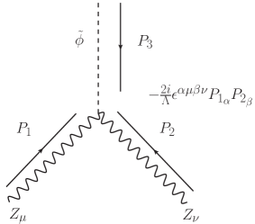
(c) $Z_{\mu}\,Z_{\nu}\,\tilde{\phi}$ vertex          

Figure 6: Gauge boson pseudo scalar vertices after EWSB

Appendix B Calculation of momentum distribution function of $\tilde{\phi}$

In this section, we have briefly discussed the calculation of momentum distribution function $f(p,T)$ of $\tilde{\phi}$ which is produced from the annihilation of SM particles and $\tilde{\phi}$ can also decay  to the DM particles. The Boltzmann equation at the level of momentum distribution function can be written as

$$\hat{L}f(p,T)=\hat{\mathcal{C}}[f(p,T)]\,,$$ (21)

where $\hat{L}=\dfrac{\partial}{\partial t}-Hp\dfrac{\partial}{\partial p}$, is the Liouville operator, $\hat{\mathcal{C}}[f(p,T)]$ is the collision term and $p\equiv|\vec{p}|$.
To simplify the form of Liouville operator, we have made the following variable transformations as in Ref. Biswas:2016iyh ; Konig:2016dzg

$$r =\dfrac{M_{0}}{T}\,.$$ (22)

$$\xi =\left(\dfrac{g_{s}(T_{0})}{g_{s}(T)}\right)^{1/3}\dfrac{p}{T}\,.$$ (23)

Where $M_{0}$ and $T_{0}$ are some reference mass and temperature scale respectively. Using the above transformations, Liouville operator takes the following form

$$\hat{L}=rH\left(1+\dfrac{1}{3}\dfrac{d\,(\ln\,g_{s}(T))}{d\,(\ln T)}\right)^{-1}\dfrac{d}{dr}\,.$$ (24)

Now substituting this expression of $\hat{L}$ in Eq.(21), we can write

$$rH\left(1+\dfrac{1}{3}\dfrac{d\,(\ln\,g_{s}(T))}{d\,(\ln T)}\right)^{-1}\dfrac{df(\xi,r)}{dr}\,=\,\hat{\mathcal{C}}[f(\xi,r)]_{\rm prod.}\,+\,\hat{\mathcal{C}}[f(\xi,r)]_{\rm decay}\,,$$ (25)

where $\hat{\mathcal{C}}[f(\xi,r)]_{\rm prod.}$ and $\hat{\mathcal{C}}[f(\xi,r)]_{\rm decay}$ are the collision terms for the production of $\tilde{\phi}$ (from annihilations and scatterings of top quark) and decay of $\tilde{\phi}$ respectively and the analytical forms are given below

$$\hat{\mathcal{C}}[f(\xi\,r)]_{\rm prod.}\,= \,\dfrac{3}{8\pi^{3}\Lambda^{2}}\left(\dfrac{m_{t}}{v}\right)^{2}\left(\dfrac{M_{0}}{r}\right)^{3}\exp\left[-\xi\,\beta(r)\right]\,\,,$$

$$\hat{\mathcal{C}}[f(\xi,r)]_{\rm decay}\,= \,-\dfrac{m_{\tilde{\phi}}\,r}{M_{0}\sqrt{\xi^{2}\beta(r)^{2}+\left(\dfrac{m_{\tilde{\phi}}\,r}{M_{0}}\right)^{2}}}f(\xi,r)\Gamma_{\tilde{\phi}\rightarrow\bar{\chi}\chi}\,\,,$$ (26)

where $\beta(r)=\left(\dfrac{g_{s}(M_{0}/r)}{g_{s}(M_{0}/r_{in})}\right)^{1/3}$. Using Eq.(26), we have solved Eq.(25) numerically to calculate the momentum distribution function of $\tilde{\phi}$.

Appendix C Calculation of the collision term for $2\rightarrow 3$ and $2\rightarrow 4$ processes

In this section,we have derived the collision term for $2\rightarrow 3$ and $2\rightarrow 4$ processes which are denoted by $\mathcal{F}_{2\rightarrow 3}(T)$ and $\mathcal{F}_{2\rightarrow 4}(T)$ respectively in Eq.(4). The forms of $\mathcal{F}_{2\rightarrow 3}(T)$ and $\mathcal{F}_{2\rightarrow 4}(T)$ are given by

$$\mathcal{F}_{2\rightarrow 3}(T)= \int\prod_{p_{i}=1}^{2}d\Pi_{p_{i}}\prod_{k_{i}=1}^{3}d\Pi_{k_{i}}\left(2\pi\right)^{4}\delta^{4}\left(\sum_{i=1}^{2}p_{i}-\sum_{i=1}^{3}k_{i}\right)\overline{|\mathcal{M}|}^{2}_{2\rightarrow 3}\exp\left(-\dfrac{E_{1}+E_{2}}{T}\right)$$ (27)

$$\mathcal{F}_{2\rightarrow 4}(T)= \int\prod_{p_{i}=1}^{2}d\Pi_{p_{i}}\prod_{k_{i}=1}^{4}d\Pi_{k_{i}}\left(2\pi\right)^{4}\delta^{4}\left(\sum_{i=1}^{2}p_{i}-\sum_{i=1}^{4}k_{i}\right)\overline{|\mathcal{M}|}^{2}_{2\rightarrow 4}\exp\left(-\dfrac{E_{1}+E_{2}}{T}\right)$$ (28)

and

$$\int d\Pi_{i}=g_{i}\int\dfrac{d^{3}\vec{p_{i}}}{(2\pi)^{3}2E_{i}}.$$

To simplify Eq.(27), we have decomposed the 3 body phase space into two 2 body phase space and the phase space integral is

$$\Phi_{3}(s)=\int_{(m_{1}+m_{2})^{2}}^{(\sqrt{s}-m_{3})^{2}}\dfrac{dX^{2}}{(2\pi)}\,\Phi_{2}(X^{2},\,m_{1}^{2},\,m_{2}^{2})\,\Phi_{2}(s,\,m_{3}^{2},\,X^{2})$$ (29)

and

$$\Phi_{2}(s,\,m_{i}^{2},\,m_{j}^{2})=\dfrac{1}{8\pi}\sqrt{1+\dfrac{m_{i}^{4}}{s^{2}}+\dfrac{m_{j}^{4}}{s^{2}}-\dfrac{2m_{i}^{2}}{s}-\dfrac{2m_{j}^{2}}{s}-\dfrac{2m_{j}^{2}m_{i}^{2}}{s^{2}}}\int\dfrac{d\Omega_{ij}}{4\pi}$$

Using Eq.(29), Eq.(27) for $2\,\rightarrow\,3$ processes ($t\,\bar{t}\rightarrow\chi\,\bar{\chi}\,\Phi$, $t\,\Phi\rightarrow\chi\,\bar{\chi}\,t$, $\bar{t}\,\Phi\rightarrow\chi\,\bar{\chi}\,\bar{t}$) can be written as

$$\mathcal{F}_{2\rightarrow 3}(T)=\dfrac{\alpha\,T}{(2\pi)^{4}}\int_{0}^{\infty}\dfrac{\sqrt{s}}{4}\left[\mathcal{A}^{\rm s-channel}_{2\rightarrow 3}(s)+2\,\mathcal{A}^{\rm t-channel}_{2\rightarrow 3}(s)\right]{\rm K}_{1}\left(\dfrac{\sqrt{s}}{T}\right)ds\,,$$ (30)

where $\mathcal{A}^{\rm s-channel}_{2\rightarrow 3}(s)$ and $\mathcal{A}^{\rm t-channel}_{2\rightarrow 3}(s)$ have the following expressions,

$$\mathcal{A}^{\rm s-channel}_{2\rightarrow 3}(s) = {s\,\ln}\,\left(\dfrac{s}{4m_{\chi}^{2}}\right)-s\,,$$

$$\mathcal{A}^{\rm t-channel}_{2\rightarrow 3}(s) = \dfrac{1}{4}\left({s\,\ln}\,\left(\dfrac{s}{4m_{\chi}^{2}}\right)-\dfrac{3}{2}s\right)\,.$$ (31)

Here $\alpha=\dfrac{1}{32\,\pi^{3}\,N_{c}}\,\left(\dfrac{g}{\Lambda}\dfrac{m_{t}}{v}\right)^{2}$ and $N_{c}=3$ is the color factor for top quark.

Similarly, for $2\,\rightarrow\,4$ process ($\Phi\,\Phi\,\rightarrow\,\chi\,\bar{\chi}\,\chi\,\bar{\chi}$)

$$\mathcal{F}_{2\rightarrow 4}(T)=\dfrac{\pi^{2}T}{(2\pi)^{6}}\int_{0}^{\infty}\sqrt{s}\,{\rm K}_{1}\left(\dfrac{\sqrt{s}}{T}\right)\mathcal{A}(s)ds\,\,\,,$$ (32)

where,

$$\mathcal{A}(s)=\dfrac{\lambda^{2}g^{4}}{8(2\pi)^{3}}\int_{0}^{s}\dfrac{dX^{2}}{2\pi}\dfrac{1}{X^{2}}\int_{0}^{(\sqrt{s}-X)^{2}}\dfrac{dY^{2}}{2\pi}\dfrac{1}{Y^{2}}\sqrt{1+\dfrac{X^{4}}{s^{2}}+\dfrac{Y^{4}}{s^{2}}-\dfrac{2X^{2}}{s}-\dfrac{2Y^{2}}{s}-\dfrac{2X^{2}Y^{2}}{s^{2}}}\,\,\,.$$

Using Eqs.(30) and (32), one can solve Eq.(4) to calculate the co-moving number density of $\chi$ from these $2\rightarrow 3$ and $2\rightarrow 4$ processes.

Appendix D Boltzmann equation for freeze-in via scattering

In this section, first we have derived a general solution of the Boltzmann equation of a dark matter candidate $\chi$ produced at the early Universe from scattering of bath particles. Such production process via freeze-in mechanism has both UV and IR contributions and particularly it depends on the type of interactions that our dark matter candidate $\chi$ has with other particles present in the Universe. After deriving a general expression of comoving number density ($Y_{\chi}$) of $\chi$ for freeze-in, we have given a more simplified expression of $Y_{\chi}$ for the case of UV freeze-in. As we have already known that for UV freeze-in one needs higher dimensional effective interactions between $\chi$ and other bath particles hence, we will consider a dimension five interaction $\dfrac{\Phi^{\dagger}\Phi\,\overline{\chi}{\chi}}{\Lambda}$ between $\chi$ and Higgs doublet $\Phi$ (the first term of Eq. (2)) as an example. Once we derive an expression of $Y_{\chi}$ for this dimension five operator, it can easily be generalised for any higher dimensional operator. Let us assume that our dark matter candidate $\chi$ is produced at the early Universe from annihilations of $\Phi$ and $\Phi^{\dagger}$ (depicted in Fig. 1).  To calculate the net number density (hence relic density) of $\chi$ generated from $\Phi^{\dagger}\Phi\rightarrow\overline{\chi}\chi$, one needs to solve the Boltzmann equation which is given by,

$$\frac{dn_{\chi}}{dt}+3Hn_{\chi}\simeq\int d\Pi_{\Phi}d\Pi_{\Phi^{\dagger}}d\Pi_{\chi}d\Pi_{\overline{\chi}}\Bigg{[}f^{\rm eq}_{\Phi}(\vec{p}_{1},T)f^{\rm eq}_{\Phi^{\dagger}}(\vec{p}_{2},T)\overline{\left|\mathcal{M}\right|}^{2}_{\Phi^{\dagger}\Phi\rightarrow\overline{\chi}\chi}(2\pi)^{4}\delta^{4}(P_{1}+P_{2}-P_{3}-P_{4})\Bigg{]}\,,$$ (33)

where $P_{1}$, $P_{2}$, $P_{3}$ and $P_{4}$ are the four momenta of $\Phi$, $\Phi^{\dagger}$, $\chi$ and $\overline{\chi}$ respectively while the corresponding three momenta are denoted by $\vec{p_{i}}$s. Besides, $d\Pi_{i}\equiv g_{i}\frac{d^{3}\vec{p_{i}}}{(2\pi)^{3}2E_{i}}$ is invariant under the Lorentz transformation and $g_{i}$ is the number of internal degrees of freedom of the particle having three momentum $\vec{p_{i}}$ while $\overline{\left|\mathcal{M}\right|}^{2}_{\Phi^{\dagger}\Phi\rightarrow\overline{\chi}\chi}$ is the Lorentz invariant matrix amplitude square for the process ${\Phi^{\dagger}\Phi\rightarrow\overline{\chi}\chi}$ and it is averaged over spins of initial and final state particles. Here we have assumed that all the particles except $\chi$ are in thermal equilibrium and they obey Maxwell Boltzmann distribution. Moreover, as the initial number densities of $\chi$ and $\overline{\chi}$ are negligible compared to those of $\Phi$ and $\Phi^{\dagger}$, we have neglected the back reaction term in the right hand side of the Boltzmann equation. To proceed further, let us define a dimensionless quantity $Y_{\chi}$ which is known as the co-moving number density $\chi$ and it is defined as $Y_{\chi}(T)=\frac{n_{\chi}(T)}{s(T)}$, where $s(T)$ is the entropy density of the Universe at temperature $T$. In terms of $Y_{\chi}(T)$ the left hand side of Eq. (33) takes the following form

$$s\frac{dY_{\chi}}{dt}\simeq\int d\Pi_{\Phi}d\Pi_{\Phi^{\dagger}}d\Pi_{\chi}d\Pi_{\overline{\chi}}\Bigg{[}f^{\rm eq}_{\Phi}(\vec{p}_{1},T)f^{\rm eq}_{\Phi^{\dagger}}(\vec{p}_{2},T)\overline{\left|\mathcal{M}\right|}^{2}_{\Phi^{\dagger}\Phi\rightarrow\overline{\chi}\chi}(2\pi)^{4}\delta^{4}(P_{1}+P_{2}-P_{3}-P_{4})\Bigg{]}\,.$$ (34)

Now, using the time-temperature relation for the radiation dominated era $\frac{dT}{dt}\simeq-HT$, the above equation can be expressed as

$$\frac{dY_{\chi}}{dT}\simeq-\frac{1}{sHT}\int d\Pi_{\Phi}d\Pi_{\Phi^{\dagger}}d\Pi_{\chi}d\Pi_{\overline{\chi}}\Bigg{[}f^{\rm eq}_{\Phi}(\vec{p}_{1},T)f^{\rm eq}_{\Phi^{\dagger}}(\vec{p}_{2},T)\overline{\left|\mathcal{M}\right|}^{2}_{\Phi^{\dagger}\Phi\rightarrow\overline{\chi}\chi}(2\pi)^{4}\delta^{4}(P_{1}+P_{2}-P_{3}-P_{4})\Bigg{]}\,,$$ (35)

where $H$ being the Hubble parameter. Now, using the definition of cross section $\sigma$ for ${\Phi^{\dagger}\Phi\rightarrow\overline{\chi}\chi}$ the collision term of the Boltzmann equation further simplifies to

$$\frac{dY_{\chi}}{dT}\simeq-\frac{1}{sHT}\int d\Pi_{\Phi}d\Pi_{\Phi^{\dagger}}4\,E_{\Phi}\,E_{\Phi^{\dagger}}\sigma\,{\rm v_{\rm rel}}\,f^{\rm eq}_{\Phi}(\vec{p}_{1},T)\,f^{\rm eq}_{\Phi^{\dagger}}(\vec{p}_{2},T)\,.$$ (36)

The integration in the right hand side is nothing but a product of two well known quantities $\langle\sigma\,{\rm v_{\rm rel}}\rangle_{\Phi^{\dagger}\Phi\rightarrow\overline{\chi}\chi}$ and $n^{\rm eq}_{\Phi}n^{\rm eq}_{\Phi^{\dagger}}$, where thermal averaged cross section and equilibrium number densities are defined as

$$\langle\sigma\,{\rm v_{\rm rel}}\rangle_{\Phi^{\dagger}\Phi\rightarrow\overline{\chi}\chi}=\dfrac{\int d\Pi_{\Phi}d\Pi_{\Phi^{\dagger}}E_{\Phi}\,E_{\Phi^{\dagger}}\sigma\,{\rm v_{\rm rel}}\,f^{\rm eq}_{\Phi}(\vec{p}_{1},T)\,f^{\rm eq}_{\Phi^{\dagger}}(\vec{p}_{2},T)}{\int d\Pi_{\Phi}d\Pi_{\Phi^{\dagger}}E_{\Phi}\,E_{\Phi^{\dagger}}f^{\rm eq}_{\Phi}(\vec{p}_{1},T)\,f^{\rm eq}_{\Phi^{\dagger}}(\vec{p}_{2},T)}\,,$$ (37)

and

$$n^{\rm eq}_{\Phi(\Phi^{\dagger})}=2\int d\Pi_{\Phi(\Phi^{\dagger})}E_{{\Phi}(\Phi^{\dagger})}\,f^{\rm eq}_{\Phi(\Phi^{\dagger})}(\vec{p}_{1(2)},T)\,.$$ (38)

Therefore, using Eqs. (37, 38), the Boltzmann equation can be written in a more compact notation as

$$\frac{dY_{\chi}}{dT}\simeq-\frac{1}{sHT}\,n^{\rm eq}_{\Phi}\,n^{\rm eq}_{\Phi^{\dagger}}\,\langle\sigma\,{\rm v_{\rm rel}}\rangle_{\Phi^{\dagger}\Phi\rightarrow\overline{\chi}\chi}\,.$$ (39)

If we assume there is no asymmetry in the number densities of $\Phi$ and $\Phi^{\dagger}$ then $n^{\rm eq}_{\Phi}=n^{\rm eq}_{\Phi^{\dagger}}$. Also, we have neglected the effect of change in number density of $\chi$ from the inverse process i.e. $\overline{\chi}\chi\rightarrow\Phi\Phi^{\dagger}$ due to insufficient number densities of $\chi$ and $\overline{\chi}$. Otherwise, we will have a term with a +ve sign and proportional to $n_{\chi}\,n_{\overline{\chi}}$ in the right hand side of the above equation. If one incorporates these two things then the above equation will reduce to the more familiar form of the Boltzmann equation. Now, following the mathematical steps given in Gondolo:1990dk for the calculation of thermal averaged cross section, one can further express the right hand side as

$$\frac{dY_{\chi}}{dT}\simeq-\frac{1}{sHT}\,\,\dfrac{g_{\Phi}^{2}\,T}{16\,\pi^{4}}\int^{\infty}_{4\,m^{2}_{\Phi}}d\hat{s}\,\sigma\,F\sqrt{\hat{s}-4\,m^{2}_{\Phi}}\,{\rm K_{1}}\left(\frac{\sqrt{\hat{s}}}{T}\right)\,.$$ (40)

Where $g_{\Phi}$ and $m_{\Phi}$ are the internal degrees of freedom and mass of $\Phi$ and ${\rm K_{1}}\left(\frac{\sqrt{s}}{T}\right)$ is the first order Modified Bessel function of second kind. The quantity $F$ is related to the initial state momentum ($\vec{\mathfrak{p}}_{i}$) in centre of momentum frame as $F=|\vec{\mathfrak{p}}_{i}|\sqrt{\hat{s}}$ with $\sqrt{\hat{s}}$ being the total energy of scattering in centre of momentum frame. Moreover, by using the standard expressions of differential cross section $\frac{d\sigma}{d\Omega}$ in centre of momentum frame, the above equation reduces to another well known form as given in Hall:2009bx ; Elahi:2014fsa ,

$$\frac{dY_{\chi}}{dT}\simeq-\frac{1}{sHT}\,\,\dfrac{g_{\Phi}^{2}\,T}{512\,\pi^{6}}\int^{\infty}_{4\,m^{2}_{\Phi}}d\hat{s}\int d\Omega\,|\vec{\mathfrak{p}}_{f}|\,|\vec{\mathfrak{p}}_{i}|\dfrac{\overline{\left|\mathcal{M}\right|}^{2}_{\Phi^{\dagger}\Phi\rightarrow\overline{\chi}\chi}}{\sqrt{\hat{s}}}\,{\rm K_{1}}\left(\frac{\sqrt{\hat{s}}}{T}\right)\,.$$ (41)

Here, $\vec{\mathfrak{p}}_{f}$ is the final state momentum in centre of momentum frame. So far, we have not used the information about the nature of interaction between dark matter and mother particles into the derivation of Boltzmann equation. Thus Eqs. (39-41) are equally applicable for both types of freeze-in where dark matter candidate $\chi$ is produced from annihilation of $\Phi$ and $\Phi^{\dagger}$. However, for the case of UV freeze-in one can further simplify the collision term of the Boltzmann equation. As mentioned in the beginning, here we will consider a dimension five operator $\dfrac{\Phi^{\dagger}\Phi\,\overline{\chi}{\chi}}{\Lambda}$. The matrix amplitude square for dark matter production process $\Phi^{\dagger}\Phi\rightarrow\overline{\chi}\chi$ is given by

$$\overline{\left|\mathcal{M}\right|}^{2}_{\Phi^{\dagger}\Phi\rightarrow\overline{\chi}\chi}=\,\dfrac{2}{\Lambda^{2}}\left(\hat{s}-4\,m^{2}_{\chi}\right)\,.$$ (42)

As UV freeze-in occurs at very early Universe when temperature $T$ is much larger compared to the masses of associated particles, in the following we consider both dark matter as well as initial state particles to be massless. Now, using the expressions of $\overline{\left|\mathcal{M}\right|}^{2}_{\Phi^{\dagger}\Phi\rightarrow\overline{\chi}\chi}$, $|\vec{\mathfrak{p}}_{i}|$ and $|\vec{\mathfrak{p}}_{f}|$ (in massless limit) in Eq. (41) we get

$$\frac{dY_{\chi}}{dT} \simeq -\frac{1}{sHT}\,\dfrac{T}{256\pi^{5}\,\Lambda^{2}}\int_{0}^{\infty}d\hat{s}\,\,\hat{s}^{3/2}\,{\rm K_{1}}\left(\frac{\sqrt{\hat{s}}}{T}\right)\,,$$ (43)

$$\simeq -\dfrac{1}{s\,H}\dfrac{T^{5}}{8\pi^{5}\Lambda^{2}}\,,$$

$$\simeq -\dfrac{45M_{pl}}{\,1.66\times 16\,\pi^{7}\sqrt{g_{\rho}}\,g_{s}\,\Lambda^{2}}\,.$$

In the last line we have used the expressions of Hubble parameter $H=\dfrac{1.66\sqrt{g_{\rho}}}{M_{pl}}T^{2}$ and entropy density $s=\dfrac{2\pi^{2}}{45}\,g_{s}T^{3}$ for radiation dominated era. Furthermore, we assume that the production of $\chi$ via UV freeze-in is effective in a period when degrees of freedoms $g_{\rho}$ and $g_{s}$ remain constant with $T$. This assumption is indeed true for our scenario where UV freeze-in occurs much before EWSB. Consequently, $\frac{dY_{\chi}}{dT}$ becomes independent of temperature $T$ and $Y_{\chi}$ depends linearly on $T$ with maximum contribution to $Y_{\chi}$ coming at the maximum possible temperature after reheating, which can be taken to be equal to the reheat temperature $T_{\rm RH}$. Therefore,

$$Y_{\chi}\simeq\dfrac{360\,M_{pl}}{\,1.66\times(2\pi)^{7}\sqrt{g_{\rho}(T_{\rm RH})}\,g_{s}(T_{\rm RH})\,\Lambda^{2}}T_{\rm RH}\,,$$ (44)

with $M_{pl}=1.22\times 10^{19}$ GeV, the Planck mass.

Appendix E Boltzmann equation for Freeze-in via decay

In this section, we have briefly discussed the Boltzmann equation of a dark matter candidate $\chi$ produced from the decay of a mother particle $\phi$ ($\phi\rightarrow\overline{\chi}{\chi}$) which is in thermal equilibrium and following Maxwell-Boltzmann distribution. The Boltzmann equation for $\chi$ in this case is given by,

$$\frac{dn_{\chi}}{dt}+3Hn_{\chi}\simeq\int d\Pi_{\phi}d\Pi_{\chi}d\Pi_{\overline{\chi}}\,\overline{\left|\mathcal{M}\right|}^{2}_{\phi\rightarrow\overline{\chi}\chi}(2\pi)^{4}\delta^{4}(P_{1}-P_{2}-P_{3})f^{\rm eq}_{\phi}(\vec{p}_{1},T)\,,$$ (45)

where, similarly to the previous case, here also we denote four momenta by $P_{i}$ and the corresponding three momenta by $\vec{p}_{i}$. Moreover, we also neglect the effect of inverse decay on $n_{\chi}$ due to non-thermal nature of $\chi$. Using the standard definition of decay width for a two body process like $\phi\rightarrow\overline{\chi}\chi$ and also the definition of $n^{\rm eq}_{\phi}$ (Eq (38)), the right hand side of the Boltzmann equation can be expressed as

$$\frac{dn_{\chi}}{dt}+3Hn_{\chi} \simeq 2\,m_{\phi}\,\Gamma_{\phi\rightarrow\overline{\chi}\chi}\,\int d\Pi_{\phi}f^{\rm eq}_{\phi}(\vec{p}_{1},T)\,,$$ (46)

$$\simeq \int\Gamma^{\prime}_{\phi\rightarrow\overline{\chi}\chi}\,f^{\rm eq}_{\phi}(\vec{p}_{1},T)\dfrac{g_{\phi}\,d^{3}\vec{p}_{1}}{(2\pi)^{3}}\,,$$

$$\simeq n^{\rm eq}_{\phi}\,\langle\Gamma\rangle_{\phi\rightarrow\overline{\chi}\chi}\,,$$

where $\Gamma_{\phi\rightarrow\overline{\chi}\chi}$ and $\Gamma^{\prime}_{\phi\rightarrow\overline{\chi}\chi}$ are partial decay widths of $\phi$ into $\overline{\chi}\chi$ final state in the rest frame of $\phi$ and in a frame where $\phi$ is moving with a four momentum $P_{1}\,(E_{1},\,\vec{p}_{1})$ respectively and $\Gamma^{\prime}_{\phi\rightarrow\overline{\chi}\chi}=\dfrac{m_{\phi}}{E_{1}}\,\Gamma_{\phi\rightarrow\overline{\chi}\chi}$. The quantity $\langle\Gamma\rangle_{\phi\rightarrow\overline{\chi}\chi}$ is thermal averaged decay width and it is defined as

$$\langle\Gamma\rangle_{\phi\rightarrow\overline{\chi}\chi}=m_{\phi}\dfrac{\int d\Pi_{\phi}\,\Gamma_{\phi\rightarrow\overline{\chi}\chi}\,f^{\rm eq}_{\phi}(\vec{p}_{1},T)}{\int d\Pi_{\phi}\,E_{1}\,f^{\rm eq}_{\phi}(\vec{p}_{1},T)}\,,$$ (47)

while the equilibrium number density $n^{\rm eq}_{\phi}$ is defined in Eq. (38). Now, in order to proceed further we have to choose a distribution function for the mother particle $\phi$. As $\phi$ is in thermal equilibrium, if we consider the Maxwell-Boltzmann distribution i.e. $f^{\rm eq}_{\phi}(\vec{p}_{1},T)=\exp(-E_{1}/T)$ then both $\langle\Gamma\rangle_{\phi\rightarrow\overline{\chi}\chi}$ and $n^{\rm eq}_{\phi}$ reduce to respective well known forms i.e. $\langle\Gamma\rangle_{\phi\rightarrow\overline{\chi}\chi}=\dfrac{{\rm K_{1}}\left(\frac{m_{\phi}}{T}\right)}{{\rm K_{2}}\left(\frac{m_{\phi}}{T}\right)}\Gamma_{\phi\rightarrow\overline{\chi}\chi}$ and $n^{\rm eq}_{\phi}=\dfrac{T}{2\pi^{2}}\,g_{\phi}\,m^{2}_{\phi}\,{\rm K_{2}}\left(\frac{m_{\phi}}{T}\right)$. Using these two expressions, one can further simplify the collision term as

$$\frac{dn_{\chi}}{dt}+3Hn_{\chi}\simeq\dfrac{g_{\phi}\,m^{2}_{\phi}\,\Gamma_{\phi\rightarrow\overline{\chi}\chi}\,T}{2\pi^{2}}\,{\rm K_{1}}\left(\frac{m_{\phi}}{T}\right)\,.$$ (48)

The left hand side of the above equation can be written as a temperature variation of comoving number density $Y_{\chi}$ following the procedure discussed in the previous section. Therefore, in terms of $Y_{\chi}$, the Boltzmann equation for freeze-in via decay has the following form

$$\frac{dY_{\chi}}{dT} \simeq -\frac{1}{sHT}\,\dfrac{g_{\phi}\,m^{2}_{\phi}\,\Gamma_{\phi\rightarrow\overline{\chi}\chi}\,T}{2\pi^{2}}\,{\rm K_{1}}\left(\frac{m_{\phi}}{T}\right)\,,$$ (49)

and

$$Y_{\chi} \simeq -\dfrac{g_{\phi}\,m^{2}_{\phi}\,\Gamma_{\phi\rightarrow\overline{\chi}\chi}}{2\pi^{2}}\int_{T_{max}}^{T_{min}}\frac{dT}{sH}\,{\rm K_{1}}\left(\frac{m_{\phi}}{T}\right)\,,$$ (50)

$$\simeq -\dfrac{45\,g_{\phi}\,m^{2}_{\phi}\,M_{pl}\,\Gamma_{\phi\rightarrow\overline{\chi}\chi}}{1.66\times 4\pi^{4}}\int_{T_{max}}^{T_{min}}dT\,\dfrac{{\rm K_{1}}\left(\frac{m_{\phi}}{T}\right)}{T^{5}\,\sqrt{g_{\rho}}\,g_{s}}\,.$$

Here also we have used the expressions of $H$ and $s$ for radiation dominated era. $T_{max}$ and $T_{min}$ are initial and final temperatures. As the integrand has maxima around $T\simeq m_{\phi}$, considering $T_{max}=\infty$ and $T_{min}=0$, one can finally get the following expression of $Y_{\chi}$,

$$Y_{\chi}\simeq\dfrac{135\,M_{pl}}{1.66\times 8\pi^{3}}\dfrac{g_{\phi}\,\Gamma_{\phi\rightarrow\overline{\chi}\chi}}{m^{2}_{\phi}\,\sqrt{g_{\rho}(m_{\phi})}\,g_{s}(m_{\phi})}\,.$$ (51)

Appendix F Calculation of X-ray flux:

Figure 7: Schematic diagram of dark matter annihilation via a long lived mediator $\tilde{\phi}$.

Let us consider two dark matter particles annihilate into two $\tilde{\phi}$s and each of them decays to two photons and further the corresponding decay of $\tilde{\phi}$ is not instantaneous. This means $\tilde{\phi}$ travels a certain distance depending on this lifetime before decaying into a pair of $\gamma$. This situation has been illustrated in Fig. 7, where the point $C$ represents the galactic centre. The annihilation of dark matter occurs at $A$ while the decay of $\tilde{\phi}$ after travelling a distance $\vec{r^{\prime}}$ happens at $B$. $O$ is the position of the earth with respect to the galactic centre. Now, in such a situation, we want to calculate the photon flux detected by a telescope placed at $O$, which is produced at $B$ from the cascade annihilations of $\chi$. First, we derive the expression of $\gamma$-ray flux for the present situation following Rothstein:2009pm ; Chu:2017vao and then we discuss how it differs from the $\gamma$-ray flux involving direct dark matter annihilation. As mentioned earlier, let two $\chi$s annihilate at $A$ to produce two $\tilde{\phi}$s and each of them decays into two $\gamma$s at $B$ while the position vectors of $A$ and $B$ with respect to the galactic centre $C$ are $\vec{x}_{s}$ and $\vec{x}$ respectively. If total number density of dark matter at $\vec{x}_{s}$ is $n_{\chi}(\vec{x}_{s})$ then the annihilation rate per $\bar{\chi}$ particle is given by,

$$\Gamma_{ann}(\vec{x}_{s}) = \langle{\sigma{\rm v_{rel}}}\rangle_{\bar{\chi}\chi\rightarrow\tilde{\phi}\tilde{\phi}}\,\,\dfrac{n_{\chi}(\vec{x}_{s})}{2}$$ (52)

$$= \langle{\sigma{\rm v_{rel}}}\rangle_{\bar{\chi}\chi\rightarrow\tilde{\phi}\tilde{\phi}}\,\,\dfrac{\rho_{\chi}(\vec{x}_{s})}{2m_{\chi}}\,.$$

Here, the 2 factor arises because of the fact that average number densities of $\chi\,\,\text{and}\,\,\bar{\chi}\,\,\text{are}\,\,\frac{n_{\chi}}{2}$. $\rho_{\chi}(\vec{x}_{s})$ is the dark matter density at a distance $\vec{x}_{s}$ from the galactic centre while ${\langle{\sigma{\rm v_{rel}}}\rangle}_{\bar{\chi}\chi\rightarrow\tilde{\phi}\tilde{\phi}}$ is the annihilation cross section for $\bar{\chi}\chi\rightarrow\tilde{\phi}\tilde{\phi}$ and it has the following expression,

$${\langle{\sigma{\rm v_{rel}}}\rangle}_{\bar{\chi}\chi\rightarrow\tilde{\phi}\tilde{\phi}}=\dfrac{g^{4}}{16\,\pi\,m_{\chi}}\dfrac{\left(m^{2}_{\chi}-m^{2}_{\tilde{\phi}}\right)^{3/2}}{\left(2\,m^{2}_{\chi}-m^{2}_{\tilde{\phi}}\right)^{2}}\,.$$ (53)

In the above we have assumed non-relativistic nature of our dark matter particles during their annihilations to $\tilde{\phi}$s. Now, an element of volume $dV_{\vec{x}_{s}}$ at $A$ contains $\frac{\rho_{\chi}(\vec{x}_{s})}{2\,m_{\chi}}dV_{\vec{x}_{s}}$ number of $\bar{\chi}$ particles. Hence the total annihilation rate at $\vec{x}_{s}$ for an element of volume $dV_{\vec{x}_{s}}$ is

$$\Gamma_{ann}^{total}(\vec{x}_{s})={\langle{\sigma{\rm v_{rel}}}\rangle}_{\bar{\chi}\chi\rightarrow\tilde{\phi}\tilde{\phi}}\,\dfrac{\rho_{\chi}(\vec{x}_{s})}{2m_{\chi}}\times\frac{\rho_{\chi}(\vec{x}_{s})}{2\,m_{\chi}}dV_{\vec{x}_{s}}\,.$$ (54)

Here from each annihilation of $\chi$ and $\bar{\chi}$ we get two pseudo scalars. Hence, the production rate of $\tilde{\phi}$ in the elemental volume $dV_{\vec{x}_{s}}$ can be written as

$$\Gamma^{\prime}_{\tilde{\phi}}(\vec{x}_{s}) = 2\times\Gamma_{ann}^{total}(\vec{x}_{s})$$ (55)

$$= \dfrac{{\langle{\sigma{\rm v_{rel}}}\rangle}_{\bar{\chi}\chi\rightarrow\tilde{\phi}\tilde{\phi}}}{2}\,\Bigg{(}\frac{\rho_{\chi}(\vec{x}_{s})}{m_{\chi}}\Bigg{)}^{2}dV_{\vec{x}_{s}}\,,$$

$$= \Gamma_{\tilde{\phi}}(\vec{x}_{s})\,dV_{\vec{x}_{s}}\,,$$

where, $\Gamma_{\tilde{\phi}}(\vec{x}_{s})$ in the right hand side denotes the production rate of $\tilde{\phi}$ per unit volume at $\vec{x}_{s}$. Now, the probability that a particle $\tilde{\phi}$ will travel a distance $r^{\prime}$ from its source point at $\vec{x}_{s}$ without decaying is given by,

$$P(r^{\prime})=e^{-\frac{r^{\prime}}{\lambda_{\tilde{\phi}}}}\,,$$ (56)

where, $\lambda_{\tilde{\phi}}$ is the decay length of $\tilde{\phi}$, which is the average distance travelled by a particle before decaying and $\lambda_{\tilde{\phi}}$ can be expressed as,

$$\lambda_{\tilde{\phi}} = {\rm v}_{\tilde{\phi}}\,\tau_{\tilde{\phi}}\,,$$ (57)

$$= {\rm v}_{\tilde{\phi}}\,\gamma_{\tilde{\phi}}\,\tau^{0}_{\tilde{\phi}}\,,$$

$$= \dfrac{\sqrt{m^{2}_{\chi}-m^{2}_{\tilde{\phi}}}}{m_{\tilde{\phi}}}\,\tau^{0}_{\tilde{\phi}}\,,$$

$$\simeq \sqrt{0.2}\times 10^{7}\left(\dfrac{\delta}{10^{-5}}\right)^{1/2}\,\left(\dfrac{\tau^{0}_{\tilde{\phi}}}{10^{20}\,{\rm s}}\right)\,\,{\rm kpc}\,,$$

where, ${\rm v}_{\tilde{\phi}}$ is the velocity of $\tilde{\phi}$ in the laboratory frame, $\gamma_{\tilde{\phi}}\simeq\frac{m_{\chi}}{m_{\tilde{\phi}}}$ (considering non-relativistic $\chi$, i.e. $E_{\chi}\simeq m_{\chi}$). Here, $\tau^{0}_{\tilde{\phi}}=1/\Gamma_{\tilde{\phi}\rightarrow\gamma\gamma}$ is the lifetime of $\tilde{\phi}$ at rest and the corresponding decay width is given by

$${\Gamma_{\tilde{\phi}\rightarrow\gamma\gamma}\,=\,\frac{m_{\tilde{\phi}}^{3}}{16\pi\Lambda^{2}}}\,\,\,.$$ (58)

The quantity $\delta$ is already defined in the previous section, expressing the mass splitting between $\chi$ and $\tilde{\phi}$. Now to calculate how many $\tilde{\phi}$ will reach at $B$ starting from $A$, we need to know the phase space distribution of $\tilde{\phi}$.

Number of $\tilde{\phi}$ which are produced within an elementary volume $dV_{\vec{x}_{s}}$ at $\vec{x}_{s}$ will cross an elementary area $dA^{\prime}$ at $\vec{x}$ in time $dt$ is given by

$$dN_{\tilde{\phi}}(\vec{x},\vec{l})=dV_{\vec{x}_{s}}\Bigg{(}\Gamma_{\tilde{\phi}}(\vec{x}_{s})dt\Bigg{)}\Bigg{(}\frac{dA^{\prime}}{4\pi|\vec{x}-\vec{x}_{s}|^{2}}\Bigg{)}\exp\left[-\frac{|\vec{x}-\vec{x}_{s}|}{\lambda_{\tilde{\phi}}}\right]\,,$$ (59)

where, $\vec{l}$ represents the direction of propagation of $\tilde{\phi}$ which is along $\vec{r^{\prime}}=\vec{x}-\vec{x}_{s}$. Moreover, without loss of any generality we have considered both $\vec{l}$ and $\vec{dA^{\prime}}$ are along the same direction. The differential flux $d\Phi_{\tilde{\phi}}$ at $\vec{x}$ is defined as

$$d\Phi_{\tilde{\phi}}(\vec{x},\vec{l})=\dfrac{d^{2}N_{\tilde{\phi}}(\vec{x},\vec{l})}{dA^{\prime}\,dt}\,,$$ (60)

and, therefore, the flux of $\tilde{\phi}$ at $\vec{x}$ is given by,

$$\Phi_{\tilde{\phi}}(\vec{x})=\dfrac{1}{4\pi}\int dV_{\vec{x}_{s}}\,{\Gamma_{\tilde{\phi}}(\vec{x}_{s})}\dfrac{\exp\left[-\frac{|\vec{x}-\vec{x}_{s}|}{\lambda_{\tilde{\phi}}}\right]}{|\vec{x}-\vec{x}_{s}|^{2}}\,.$$ (61)

Finally, we have defined a quantity $f_{\tilde{\phi}}(\vec{x})$, called the density function of $\tilde{\phi}$ at $\vec{x}$ as

$$f_{\tilde{\phi}}(\vec{x}) = \dfrac{\Phi_{\tilde{\phi}}(\vec{x})}{{\rm v}_{\tilde{\phi}}}\,,$$ (62)

$$= \dfrac{1}{4\pi\,{\rm v}_{\tilde{\phi}}}\int dV_{\vec{x}_{s}}\,{\Gamma_{\tilde{\phi}}(\vec{x}_{s})}\dfrac{\exp\left[-\frac{|\vec{x}-\vec{x}_{s}|}{\lambda_{\tilde{\phi}}}\right]}{|\vec{x}-\vec{x}_{s}|^{2}}\,.$$

The angular distribution of photon is isotropic in the rest frame of $\tilde{\phi}$ (since the scalar is a spin zero object). However, in the galactic frame the emitted photons have some angular distribution. Let $\vec{k}$ be the direction of emitted photons (i.e.  along the position vector $-\vec{r}$ in Fig. 7) then the angular distribution of photons will depend on the angle between $\vec{l}$ and $\vec{k}$. If $dN_{\gamma}$ is the number of photons emitted along the direction $\vec{k}$ within a solid angle $d\Omega_{\gamma}$ and having energy between $E_{\gamma}$ and $E_{\gamma}+dE_{\gamma}$, then let us define a function $\mathcal{G}(\vec{k}-\vec{l},E_{\gamma})$ as

$$\mathcal{G}(\vec{k}-\vec{l},E_{\gamma})=\frac{d^{2}N_{\gamma}}{dE_{\gamma}\,d\Omega_{\gamma}}\,.$$ (63)

Therefore, the number of photons coming towards the earth in time $dt$ along the direction $\vec{k}$ from an elementary volume $dV$ situated at ${\vec{x}}$ with respect to the galactic centre is

$$dN_{\gamma}=dV\Bigg{(}\frac{dt}{\tau_{\tilde{\phi}}}f_{\tilde{\phi}}(\vec{x})\Bigg{)}\Bigg{(}\mathcal{G}(\vec{k}-\vec{l},E_{\gamma})\,dE_{\gamma}\,\frac{dA}{|\vec{x}-\vec{r}_{\odot}|^{2}}\Bigg{)}\,,$$ (64)

where $dA$ is an elementary area placed on the earth (i.e. at $O$, the position of telescope) and similar to the previous case, here also we have considered that the photons are coming along the normal to the area $dA$. Furthermore, from Fig. 7 we can write $\vec{r}=\vec{x}-\vec{r}_{\odot}$ where $\vec{r}_{\odot}$ describes the position of the earth with respect to the galactic centre. Now, using the definition of differential flux given in Eq. (60), one can easily calculate the total photon flux from the decay of $\tilde{\phi}$ as

$$\Phi_{\gamma}=\int\,\dfrac{f_{\tilde{\phi}}(\vec{x})}{\tau_{\tilde{\phi}}}\mathcal{G}(\vec{k}-\vec{l},E_{\gamma})\,\frac{dE_{\gamma}}{|\vec{x}-\vec{r}_{\odot}|^{2}}\,dV.$$ (65)

The differential photon flux on the earth can be obtained using $\vec{r}=\vec{x}-\vec{r}_{\odot}$ as

$$\frac{d^{2}\Phi_{\gamma}}{dE_{\gamma}\,d\Omega}=\frac{1}{\tau_{\tilde{\phi}}}\int_{l.o.s}dr\,f_{\tilde{\phi}}(\vec{x})\,\mathcal{G}(\vec{k}-\vec{l},E_{\gamma})\,,$$ (66)

where $\int d\Omega=\Delta\Omega$ is the field of view of the telescope placed at O. The above integration over $r$ is along the line of sight ($l.o.s$) distance. Now substituting the expression of $f_{\tilde{\phi}}(\vec{x})$ in the above we get,

$$\frac{d^{2}\Phi_{\gamma}}{dE_{\gamma}\,d\Omega}=\frac{1}{4\pi{\rm v}_{\tilde{\phi}}\tau_{\tilde{\phi}}}\int_{l.o.s}dr\int dV_{\vec{x}_{s}}{\Gamma_{\tilde{\phi}}(\vec{x}_{s})}\dfrac{\exp\left[-\frac{|\vec{x}-\vec{x}_{s}|}{\lambda_{\tilde{\phi}}}\right]}{|\vec{x}-\vec{x}_{s}|^{2}}\,\mathcal{G}(\vec{k}-\vec{l},E_{\gamma})\,.$$ (67)

Finally, using Eqs. (55, 57) the expression of photon flux is

$$\frac{d^{2}\Phi_{\gamma}}{dE_{\gamma}\,d\Omega} = \frac{1}{4\pi\lambda_{\tilde{\phi}}}\int_{l.o.s}dr\int dV_{\vec{x}_{s}}\dfrac{{\langle{\sigma{\rm v_{rel}}}\rangle}_{\bar{\chi}\chi\rightarrow\tilde{\phi}\tilde{\phi}}}{2}\,\Bigg{(}\frac{\rho_{\chi}(\vec{x}_{s})}{m_{\chi}}\Bigg{)}^{2}\dfrac{\exp\left[-\frac{|\vec{x}-\vec{x}_{s}|}{\lambda_{\tilde{\phi}}}\right]}{|\vec{x}-\vec{x}_{s}|^{2}}\,\mathcal{G}(\vec{k}-\vec{l},E_{\gamma})\,,$$ (68)

$$= \dfrac{{\langle{\sigma{\rm v_{rel}}}\rangle}_{\bar{\chi}\chi\rightarrow\tilde{\phi}\tilde{\phi}}}{2\,m^{2}_{\chi}}\int_{l.o.s}dr\,\rho^{2}_{\rm eff}(x)\,\mathcal{G}(\vec{k}-\vec{l},E_{\gamma})\,,$$

where

$$\rho^{2}_{\rm eff}(x)=\int dV_{\vec{x}_{s}}\frac{\rho^{2}_{\chi}(\vec{x}_{s})}{4\pi\lambda_{\tilde{\phi}}}\dfrac{\exp\left[-\frac{|\vec{x}-\vec{x}_{s}|}{\lambda_{\tilde{\phi}}}\right]}{|\vec{x}-\vec{x}_{s}|^{2}}\,,$$ (69)

is the square of effective dark matter density at point B. In the present case, dark matter candidate $\chi$ is non-relativistic and the mass of $\chi$ and $\tilde{\phi}$ are required to be almost degenerate to generate a line-like photon spectrum. Consequently, the intermediate particles $\tilde{\phi}$ are also non-relativistic and hence the photon spectrum will appear isotropic to the observer at the earth as well. Therefore, one can take $\mathcal{G}(\vec{k}-\vec{l},E_{\gamma})\simeq\dfrac{1}{4\pi}\dfrac{dN_{\gamma}}{dE_{\gamma}}$ and the differential photon flux from the cascade annihilation of dark matter reduces to the familiar form

$$\frac{d\Phi_{\gamma}}{dE_{\gamma}} = 2\times\dfrac{1}{4}\,\dfrac{r_{\odot}}{4\pi}\left(\dfrac{\rho_{\odot}}{m_{\chi}}\right)^{2}{\langle{\sigma{\rm v_{rel}}}\rangle}_{\bar{\chi}\chi\rightarrow\tilde{\phi}\tilde{\phi}}\,\dfrac{dN_{\gamma}}{dE_{\gamma}}\,J_{\rm eff}\Delta{\Omega}\,.$$ (70)

References

- (1) WMAP collaboration, G. Hinshaw et al., Nine-Year Wilkinson Microwave Anisotropy Probe (WMAP) Observations: Cosmological Parameter Results, Astrophys. J. Suppl. 208 (2013) 19, [1212.5226].
- (2) Planck collaboration, N. Aghanim et al., Planck 2018 results. VI. Cosmological parameters, 1807.06209.
- (3) L. Roszkowski, E. M. Sessolo and S. Trojanowski, WIMP dark matter candidates and searches—current status and future prospects, Rept. Prog. Phys. 81 (2018) 066201, [1707.06277].
- (4) XENON collaboration, E. Aprile et al., Dark Matter Search Results from a One Ton-Year Exposure of XENON1T, Phys. Rev. Lett. 121 (2018) 111302, [1805.12562].
- (5) XENON collaboration, E. Aprile et al., Physics reach of the XENON1T dark matter experiment, JCAP 1604 (2016) 027, [1512.07501].
- (6) LUX-ZEPLIN collaboration, D. S. Akerib et al., Projected WIMP Sensitivity of the LUX-ZEPLIN (LZ) Dark Matter Experiment, 1802.06039.
- (7) DARWIN collaboration, J. Aalbers et al., DARWIN: towards the ultimate dark matter detector, JCAP 1611 (2016) 017, [1606.07001].
- (8) C. Bœhm, D. G. Cerdeño, P. A. N. Machado, A. Olivares-Del Campo and E. Reid, How high is the neutrino floor?, JCAP 1901 (2019) 043, [1809.06385].
- (9) L. J. Hall, K. Jedamzik, J. March-Russell and S. M. West, Freeze-In Production of FIMP Dark Matter, JHEP 03 (2010) 080, [0911.1120].
- (10) F. Elahi, C. Kolda and J. Unwin, UltraViolet Freeze-in, JHEP 03 (2015) 048, [1410.6157].
- (11) J. McDonald, Warm Dark Matter via Ultra-Violet Freeze-In: Reheating Temperature and Non-Thermal Distribution for Fermionic Higgs Portal Dark Matter, JCAP 1608 (2016) 035, [1512.06422].
- (12) S.-L. Chen and Z. Kang, On UltraViolet Freeze-in Dark Matter during Reheating, JCAP 1805 (2018) 036, [1711.02556].
- (13) C. E. Yaguna, The Singlet Scalar as FIMP Dark Matter, JHEP 08 (2011) 060, [1105.1654].
- (14) M. Blennow, E. Fernandez-Martinez and B. Zaldivar, Freeze-in through portals, JCAP 1401 (2014) 003, [1309.7348].
- (15) A. Biswas, D. Majumdar and P. Roy, Nonthermal two component dark matter model for Fermi-LAT -ray excess and 3.55 keV X-ray line, JHEP 04 (2015) 065, [1501.02666].
- (16) R. T. Co, F. D’Eramo, L. J. Hall and D. Pappadopulo, Freeze-In Dark Matter with Displaced Signatures at Colliders, JCAP 1512 (2015) 024, [1506.07532].
- (17) B. Shakya, Sterile Neutrino Dark Matter from Freeze-In, Mod. Phys. Lett. A31 (2016) 1630005, [1512.02751].
- (18) A. Biswas and A. Gupta, Freeze-in Production of Sterile Neutrino Dark Matter in U(1)B-L Model, JCAP 1609 (2016) 044, [1607.01469].
- (19) J. König, A. Merle and M. Totzauer, keV Sterile Neutrino Dark Matter from Singlet Scalar Decays: The Most General Case, JCAP 1611 (2016) 038, [1609.01289].
- (20) A. Biswas, S. Choubey and S. Khan, FIMP and Muon () in a U Model, JHEP 02 (2017) 123, [1612.03067].
- (21) N. Bernal, M. Heikinheimo, T. Tenkanen, K. Tuominen and V. Vaskonen, The Dawn of FIMP Dark Matter: A Review of Models and Constraints, Int. J. Mod. Phys. A32 (2017) 1730023, [1706.07442].
- (22) A. Biswas, S. Choubey and S. Khan, Neutrino mass, leptogenesis and FIMP dark matter in a model, Eur. Phys. J. C77 (2017) 875, [1704.00819].
- (23) M. Pandey, D. Majumdar and K. P. Modak, Two Component Feebly Interacting Massive Particle (FIMP) Dark Matter, JCAP 1806 (2018) 023, [1709.05955].
- (24) A. Biswas, D. Borah and A. Dasgupta, UV complete framework of freeze-in massive particle dark matter, Phys. Rev. D99 (2019) 015033, [1805.06903].
- (25) D. Borah, B. Karmakar and D. Nanda, Common Origin of Dirac Neutrino Mass and Freeze-in Massive Particle Dark Matter, JCAP 1807 (2018) 039, [1805.11115].
- (26) A. Biswas and A. Gupta, Calculation of Momentum Distribution Function of a Non-thermal Fermionic Dark Matter, JCAP 1703 (2017) 033, [1612.02793].
- (27) E. Bulbul, M. Markevitch, A. Foster, R. K. Smith, M. Loewenstein and S. W. Randall, Detection of An Unidentified Emission Line in the Stacked X-ray spectrum of Galaxy Clusters, Astrophys. J. 789 (2014) 13, [1402.2301].
- (28) A. Boyarsky, O. Ruchayskiy, D. Iakubovskyi and J. Franse, Unidentified Line in X-Ray Spectra of the Andromeda Galaxy and Perseus Galaxy Cluster, Phys. Rev. Lett. 113 (2014) 251301, [1402.4119].
- (29) A. Boyarsky, J. Franse, D. Iakubovskyi and O. Ruchayskiy, Checking the Dark Matter Origin of a 3.53 keV Line with the Milky Way Center, Phys. Rev. Lett. 115 (2015) 161301, [1408.2503].
- (30) T. E. Jeltema and S. Profumo, Discovery of a 3.5 keV line in the Galactic Centre and a critical look at the origin of the line across astronomical targets, Mon. Not. Roy. Astron. Soc. 450 (2015) 2143–2152, [1408.1699].
- (31) O. Urban, N. Werner, S. W. Allen, A. Simionescu, J. S. Kaastra and L. E. Strigari, A Suzaku Search for Dark Matter Emission Lines in the X-ray Brightest Galaxy Clusters, Mon. Not. Roy. Astron. Soc. 451 (2015) 2447–2461, [1411.0050].
- (32) N. Cappelluti, E. Bulbul, A. Foster, P. Natarajan, M. C. Urry, M. W. Bautz et al., Searching for the 3.5 keV Line in the Deep Fields with Chandra: the 10 Ms observations, Astrophys. J. 854 (2018) 179, [1701.07932].
- (33) J. Jaeckel, J. Redondo and A. Ringwald, 3.55 keV hint for decaying axionlike particle dark matter, Phys. Rev. D89 (2014) 103511, [1402.7335].
- (34) H. M. Lee, S. C. Park and W.-I. Park, Cluster X-ray line at from axion-like dark matter, Eur. Phys. J. C74 (2014) 3062, [1403.0865].
- (35) J.-C. Park, S. C. Park and K. Kong, X-ray line signal from 7 keV axino dark matter decay, Phys. Lett. B733 (2014) 217–220, [1403.1536].
- (36) K.-Y. Choi and O. Seto, X-ray line signal from decaying axino warm dark matter, Phys. Lett. B735 (2014) 92–94, [1403.1782].
- (37) C. Kolda and J. Unwin, X-ray lines from R-parity violating decays of keV sparticles, Phys. Rev. D90 (2014) 023535, [1403.5580].
- (38) N. E. Bomark and L. Roszkowski, 3.5 keV x-ray line from decaying gravitino dark matter, Phys. Rev. D90 (2014) 011701, [1403.6503].
- (39) S. P. Liew, Axino dark matter in light of an anomalous X-ray line, JCAP 1405 (2014) 044, [1403.6621].
- (40) K. S. Babu and R. N. Mohapatra, 7 keV Scalar Dark Matter and the Anomalous Galactic X-ray Spectrum, Phys. Rev. D89 (2014) 115011, [1404.2220].
- (41) K. P. Modak, 3.5 keV X-ray Line Signal from Decay of Right-Handed Neutrino due to Transition Magnetic Moment, JHEP 03 (2015) 064, [1404.3676].
- (42) S. Chakraborty, D. K. Ghosh and S. Roy, 7 keV Sterile neutrino dark matter in lepton number model, JHEP 10 (2014) 146, [1405.6967].
- (43) S. Patra, N. Sahoo and N. Sahu, Dipolar dark matter in light of the 3.5 keV x-ray line, neutrino mass, and LUX data, Phys. Rev. D91 (2015) 115013, [1412.4253].
- (44) G. Arcadi, L. Covi and F. Dradi, 3.55 keV line in Minimal Decaying Dark Matter scenarios, JCAP 1507 (2015) 023, [1412.6351].
- (45) D. Borah, A. Dasgupta and R. Adhikari, Common origin of the 3.55 keV x-ray line and the Galactic Center gamma-ray excess in a radiative neutrino mass model, Phys. Rev. D92 (2015) 075005, [1503.06130].
- (46) A. Biswas, D. Majumdar and P. Roy, Dwarf galaxy -excess and 3.55 keV X-ray line in a nonthermal Dark Matter model, EPL 113 (2016) 29001, [1507.04543].
- (47) D. Borah, A. Dasgupta and S. Patra, Common origin of keV x-ray line and gauge coupling unification with left-right dark matter, Phys. Rev. D96 (2017) 115019, [1604.01929].
- (48) A. Dutta Banik, M. Pandey, D. Majumdar and A. Biswas, Two component WIMP–FImP dark matter model with singlet fermion, scalar and pseudo scalar, Eur. Phys. J. C77 (2017) 657, [1612.08621].
- (49) A. Biswas, S. Choubey, L. Covi and S. Khan, Explaining the 3.5 keV X-ray Line in a Extension of the Inert Doublet Model, JCAP 1802 (2018) 002, [1711.00553].
- (50) K. J. Bae, A. Kamada, S. P. Liew and K. Yanagi, Light axinos from freeze-in: production processes, phase space distributions, and Ly- forest constraints, JCAP 1801 (2018) 054, [1707.06418].
- (51) C. Dessert, N. L. Rodd and B. R. Safdi, Evidence against the decaying dark matter interpretation of the 3.5 keV line from blank sky observations, 1812.06976.
- (52) E. Dudas, L. Heurtier and Y. Mambrini, Generating X-ray lines from annihilating dark matter, Phys. Rev. D90 (2014) 035002, [1404.1927].
- (53) S. Baek, P. Ko and W.-I. Park, The 3.5 keV X-ray line signature from annihilating and decaying dark matter in Weinberg model, [1405.3730].
- (54) V. Brdar, J. Kopp, J. Liu and X.-P. Wang, X-Ray Lines from Dark Matter Annihilation at the keV Scale, Phys. Rev. Lett. 120 (2018) 061301, [1710.02146].
- (55) K. J. H. Phillips, B. Sylwester and J. Sylwester, THE X-RAY LINE FEATURE AT 3.5 KeV IN GALAXY CLUSTER SPECTRA, Astrophys. J. 809 (2015) 50, [1507.04619].
- (56) D. Iakubovskyi, Checking the potassium origin of the new emission line at 3.5 keV using the K xix line complex at 3.7 keV, Mon. Not. Roy. Astron. Soc. 453 (2015) 4097–4101, [1507.02857].
- (57) A. Ibarra, S. Lopez Gehler and M. Pato, Dark matter constraints from box-shaped gamma-ray features, JCAP 1207 (2012) 043, [1205.0007].
- (58) V. D. Barger and R. J. N. Phillips, COLLIDER PHYSICS. REDWOOD CITY, USA: ADDISON-WESLEY (1987) 592 P. (FRONTIERS IN PHYSICS, 71), 1987.
- (59) P. Gondolo and G. Gelmini, Cosmic abundances of stable particles: Improved analysis, Nucl. Phys. B360 (1991) 145–179.
- (60) J. Edsjo and P. Gondolo, Neutralino relic density including coannihilations, Phys. Rev. D56 (1997) 1879–1894, [hep-ph/9704361].
- (61) D. Cadamuro and J. Redondo, Cosmological bounds on pseudo Nambu-Goldstone bosons, JCAP 1202 (2012) 032, [1110.2895].
- (62) E. W. Kolb and M. S. Turner, The Early Universe, Front. Phys. 69 (1990) 1–547.
- (63) M. Bauer, M. Neubert and A. Thamm, Collider Probes of Axion-Like Particles, JHEP 12 (2017) 044, [1708.00443].
- (64) J. F. Navarro, C. S. Frenk and S. D. M. White, A Universal density profile from hierarchical clustering, Astrophys. J. 490 (1997) 493–508, [astro-ph/9611107].
- (65) M. J. L. Turner et al., The European Photon Imaging Camera on XMM-Newton: The MOS cameras, Astron. Astrophys. 365 (2001) L27–35, [astro-ph/0011498].
- (66) I. Z. Rothstein, T. Schwetz and J. Zupan, Phenomenology of Dark Matter annihilation into a long-lived intermediate state, JCAP 0907 (2009) 018, [0903.3116].
- (67) X. Chu, S. Kulkarni and P. Salati, Dark matter indirect signals with long-lived mediators, JCAP 1711 (2017) 023, [1706.08543].