Comparison of Classical Machine Learning Approaches on Bangla Textual Emotion Analysis

Abstract

Detecting emotions from text is an extension of simple sentiment polarity detection. Instead of considering only positive or negative sentiments, emotions are conveyed using more tangible manner; thus, they can be expressed as many shades of gray. This paper manifests the results of our experimentation for fine-grained emotion analysis on Bangla text. We gathered and annotated a text corpus consisting of user comments from several Facebook groups regarding socio-economic and political issues, and we made efforts to extract the basic emotions (sadness, happiness, disgust, surprise, fear, anger) conveyed through these comments. Finally, we compared the results of the five most popular classical machine learning techniques namely Naïve Bayes, Decision Tree, k-Nearest Neighbor (k-NN), Support Vector Machine (SVM) and K-Means Clustering with several combinations of features. Our best model (SVM with a non-linear radial-basis function (RBF) kernel) achieved an overall average accuracy score of 52.98% and an F1 score (macro) of 0.3324.

1 Introduction

Sentiment analysis or opinion mining is the task of automatically analyzing text documents using computational methods to obtain the opinions of the authors about specific entities, such as people, companies, events or products. At present, the web has become an excellent source of opinions about entities, particularly with the increased popularity of social media. People are expressing their opinions through reviews, forum discussions, blogs, tweets, comments and posts. Individuals and organizations are increasingly using these opinions for decision-making purposes.

Thus we took an initiative that aims at developing and annotating a text corpus in Bangla for doing fine-grained emotion analysis. The term Emotion Analysis is used because instead of dividing the corpus based on only positive and negative sentiments, we tried to consider more fine-grained emotion labels such as sadness, happiness, disgust, surprise, fear and anger - which are, according to Paul Ekman Ekman (1999), the six basic emotion categories. Next, we tried to implement five different classical machine learning algorithms, namely the Naïve Bayes, Decision Tree, k-Nearest Neighbours, Support Vector Machine and K-Means clustering on our corpus. Thus the contributions of this paper can briefly be seen in three major folds:

1. We will present a manually annotated Bangla emotion corpus, which incorporates the diversity of fine-grained emotion expressions in social-media text.

2. We will employ classical machine-learning approaches that typically perform well in classifying the six aforementioned emotion types.

3. We will compare the machine-learning classifiers’ performance with a baseline to identify the best-performing model for fine-grained emotion classification.

Using our own carefully curated gold standard corpus, we will report our preliminary efforts to train and evaluate machine learning models for emotion classification in Bangla text. Our experimental results show that a non-linear SVM achieved the best performance with an accuracy score of 0.5298, and an F-score of 0.3324 (macro) and 0.476 (micro) among all the tested classifiers.

2 Related Works

To our knowledge, the reliable literature on fine-grained emotion tagging for Bangla is very limited. For example, a reliable research work was that of Das and Bandyopadhyay Das and Bandyopadhyay (2010b). In their work, they annotated a random collection of 123 blog posts consisting a total of 12,149 sentences. The task was mainly focused on observing the performance of different machine learning classifiers. On a small subset of 200 test sentences, the Conditional Random Field (CRF) achieved an average accuracy of 0.587 whereas the SVM scored 0.704.

In a different paper Das and Bandyopadhyay (2010a), the authors described the preparation of the Bengali WordNet Affect containing six types of emotion words. They employed an automatic method of sense disambiguation. The Bengali WordNet Affect could be useful for emotion-related language processing tasks in Bengali.

In his paper, Das Das (2011) delineates the identification of the emotional contents at a document-level along with their associated holders and topics. Additionally, he manually annotated a small corpus. By applying sense-based affect-estimation techniques, he gained a micro F-score of 0.66 and 0.619 in terms of ‘emotion holder’ and ‘emotion topic’ identification.

On a case study for Bengali Das et al. (2012), the authors considered 1,100 sentences on eight different topics. They prepared a knowledge base for emoticons and also employed a morphological analyzer to identify the lexical keywords from the Bengali WordNet Affect lists. They claimed an overall precision, recall and F1-Score (micro) of 0.594, 0.65 and 0.653 respectively.

Jasy and Howard Liew and Turtle (2016) investigated certain prevalent machine learning techniques on coarse-grained emotions for English. They used the grounded-theory method to construct a corpus of 5,553 tweets, manually annotated with 28 emotion categories. They showed that SVM and BayesNet outperformed all the classifiers. The BayesNet correctly predicted roughly 60% of the instances, whereas the SVM was correct on 50% of the cases.

3 Data Set

We used two different datasets in our experiment. The first was the Part-of-Speech (POS) Tagset: Bengali Dandapat et al. (2009) for POS-tagging. The dataset that we were able to obtain contained approximately 3K sentences and 42K words in it’s original form, and it contained a broad category of 32 tagsets.

For the task of the Bangla emotion classification, we annotated 6,314 comments from three different Facebook groups. These comments were mostly reactions to ongoing socio-political issues and concerned the success and failure of the Bangladesh government.

3.1 Distribution of the Emotion Dataset

For the purpose of our experiment, we took a balanced set from the aforementioned data and divided it into a training and a test set of an equal ratio. We considered a proportion of 5:1 for training and evaluation purposes. Table 1 summarizes this distribution.

Labels	Training Set	Testing Set
sad	1000	200
happy	1500	300
disgust	500	100
surprise	400	80
fear	300	60
angry	1000	200
Total	4700	940

Table 1: Distribution of emotion classes in the dataset.

4 Experimental Settings and Methodology

In this section, we will describe the preprocessing and feature-selection techniques, including the POS tagging approach that we have considered for the emotion recognition models. Finally, the baseline setting for evaluation and further model optimization will be introduced.

4.1 Preprocessing and Features

Apart from cleaning the data, we also used certain simple text preprocessing techniques. We tokenized the words using a specialized tokenizer for Bangla from spaCy Honnibal and Montani (2017). Moreover, we experimented by filtering out stop words.

We have explored two types of feature vectors namely the count vectorizer and a tf-idf vectorizer with a combination of n-grams (ranging from unigrams to trigrams) from scikit-learn Pedregosa et al. (2011). Furthermore, we investigated the effect of POS tagging for feature reduction on our best model.

4.2 POS Tagging

For the purpose of POS tagging, we implemented a Hidden Markov Model (HMM) based tagger. The original POS tagger is capable of tagging 32 tags with an accuracy of 75% over the Bangla dataset (Section 3). By looking upon several combinations, we only considered five tags (‘JJ’, ‘CX’, ‘VM’, ‘NP’ and ‘AMN’) that were the most significant to emotion-related words.

4.3 Baseline Classifier

As baseline measure, we used a k-NN classifier with word unigrams plus count as features. The value of k-nearest neighbours was set to 15 (k=15). For evaluation, we will compare the results of this baseline model with the optimized model for each of the classifiers in Section 5.

5 Results and Evaluation

For the evaluation, we will first delineate the results of our baseline classifier (k-NN). Then, we will attempt to find the best model based on the results obtained in Section 5.1 through 5.6.

5.1 Baseline Performance

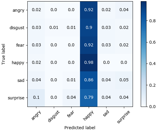
Table 2 lists in detail the results of the baseline model, whereas Table 3 summarizes the overall accuracy and the F1(macro) score.

Labels	Precision	Recall	F1(micro)
angry	0.125	0.020	0.034
disgust	1.000	0.010	0.020
fear	0.000	0.000	0.000
happy	0.342	0.977	0.507
sad	0.421	0.040	0.073
surprise	0.125	0.037	0.058
Average	0.342	0.329	0.192

Table 2: Results of K-NN Classifier as the Baseline Model with K=15.

Evaluation Matrix	Score
Accuracy	0.329
F1(macro)	0.115

Table 3: Average score of the Baseline Model.

Figure 1: Confusion Matrix (Accuracy) for Baseline.

From Table 2 and Fig. 1, it may be observed that the baseline classifier predicts almost every class as being ‘happy’. This could be the result of the classifier being biased towards this particular label because the maximum number in the training example was supplied for the category ‘happy’.

5.2 K-Nearest Neighbours

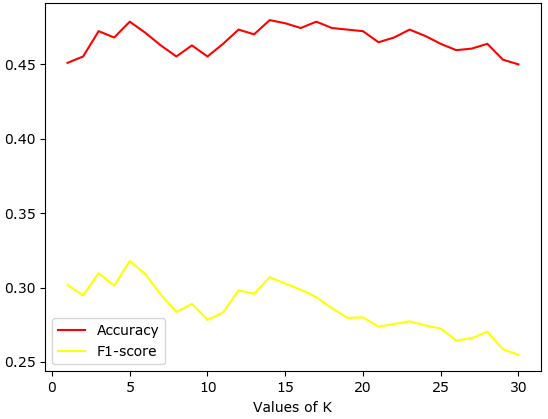
Although the baseline k-NN model performed quite poorly, we attempted to tune the parameters for the K-NN classifier to identify the best k-value for our data. Table 4 and Fig. 2 presents the results of the k-NN classifier for various k-values. It should be noted that here, we only considered the tf-idf feature because it yielded better results than the count feature. Considering the data and the plot (Fig 2), it is obvious that the classifier produces the best outputs for the k value of 5.

K-Values	Accuracy	F1(macro)
2	0.455	0.295
3	0.472	0.31
4	0.468	0.301
5	0.479	0.318
6	0.471	0.309
7	0.463	0.295

Table 4: Results of K-NN Classifier with Tf-Idf Feature for Different k-values.

Figure 2: Plot of accuracy and F1-score(macro) for different values of k.

We selected the value of k=5 as our default parameter to be further examined with different preprocessing and feature combinations (Table 5). The results indicate that the best k-NN model uses the tf-idf unigram as a feature (accuracy = 0.479, F1-macro = 0.318).

Feature	Accuracy	F1(macro)
unigram + count	0.359	0.172
unigram + tf-idf	0.479	0.318
stopword + tf-idf	0.332	0.133
stopword + count	0.342	0.146
stopword + tf-idf + n-gram(1,3)	0.316	0.091
stopword + count + n-gram(1,3)	0.330	0.114

Table 5: Results of K-NN Classifier for Different Feature Combinations (K=5).

5.3 Naïve Bayes

For our second classification algorithm, we used the ‘Multinomial Naive Bayes’ (MNB) classifier. Unlike certain other classifiers, the MNB did not require setting and tuning the parameters. Thus, we directly experimented with different feature/preprocessing techniques (Table 6).

Feature	Accuracy	F1(macro)
unigram + tf-idf	0.491	0.266
unigram + count	0.525	0.295
stopword + tf-idf	0.472	0.250
stopword + Count	0.506	0.284
n-gram(1,3) + tf-idf	0.444	0.227
n-gram(1,3) + count	0.516	0.287
stopword + tf-idf + n-gram(1,3)	0.434	0.219
stopword + count + n-gram(1,3)	0.515	0.292

Table 6: Results of Multinomial Naïve Bayes Classifier for Different Feature Combinations.

Based on the above results, the best MNB model was achieved by combining the count with the unigram feature; an accuracy score of 0.525 and an F1-macro of 0.295 were obtained during the test.

5.4 Decision Tree

The DT constructs a regression or classification model by following a tree structure. Here, optimal parameter settings were found by considering a minimum samples split of 2, minimum sample leaf size of 1. We did not impose any restrictions on the number of features and to the depth of the tree. Table 7 lists the results of several combinations of features and preprocessing schemes.

Feature	Accuracy	F1(macro)
unigram + tf-idf	0.442	0.301
unigram + count	0.432	0.287
stopword + tf-idf	0.416	0.283
stopword + count	0.430	0.292
stopword + tf-idf + n-gram(1,3)	0.394	0.247
stopword + count + n-gram(1,3)	0.421	0.277

Table 7: Results of Decision Tree Classifier for Different Feature Combinations.

According to the aforementioned results, the best DT model with an accuracy of 0.442 and an F1(macro) of 0.301 was obtained from the unigram and tf-idf combination.

5.5 K-Means Clustering

The only unsupervised machine learning approach that we used in our experiment was the K-Means Clustering. We selected a cluster size of N=6, as we have six different emotion categories. We investigated different initialization ranging from 1 to 15. Here, the initialization (n_init) is the number of times the k-means algorithm executes with different centroid seeds. The final results would be the best output of n consecutive runs. To evaluate the clustering, we used two measures: Adjusted Rand-Index and V-measure (similar to F-measure).

Feature	Adjusted Rand	V-measure
unigram + tf-idf	0.008	0.042
unigram + count	0.009	0.009
n-gram (1,3) + tf-idf	0.059	0.049
n-gram (1,3) + count	0.009	0.011

Table 8: Results of K-Means Clustering Algorithm for Different Feature Combinations

Table 8 lists the best evaluation scores for the k-means clustering model (for n_init of 1 to 15). From the results, we can see that the highest score of 0.049 in terms of the V-measure and an Adjusted Rand-Index score of 0.059 was achieved using a combination of ngram(1,3) and tf-idf feature.

5.6 Support Vector Machine

To find the best SVM-model, we used both linear and non-linear SVM-kernel. In both cases, the most important words (tf-idf) were used as features because it leads to the highest performance. We explored different values for Gamma and C-parameters and found that the non-linear kernel performed slightly better. Results and settings for the SVM model will be discussed in Section 5.7.

5.7 Best Model

Among all models, the best model was the ‘SVM with a Non-Linear RBF-Kernel’. Next, we continued experimenting with different preprocessing and feature combinations using this SVM model. Table 9 summarizes an overview of different combinations of feature and preprocessing techniques on the non-linear SVM model with an RBF-kernel. The most optimal parameter settings in this experiment were a C-parameter value of 2.0 and a Gamma-value of 0.6. The best combination of features was the most important (tf-idf) word unigrams. Therefore, the highest accuracy score achieved from the model was 0.5298 (i.e., an improvement of 20.08% from the baseline model) and an F1(macro) of 0.3324 (i.e., an improvement of 0.2174 from baseline model).

Feature	Gamma	Accuracy	F1 (macro)
POS + unigram + tf-idf	0.6	0.399	0.226
unigram + tf-idf	0.6	0.5298	0.3324
unigram + stopword + tf-idf	0.3	0.517	0.312
n-gram(1,3) + tf-idf	0.8	0.516	0.307
n-gram(1,3) + tf-idf + POS	0.8	0.399	0.224
n-gram(1,3) + stopword + tf-idf	0.4	0.525	0.313
n-gram(1,3) + stopword + tf-idf + POS	0.4	0.374	0.186
Feature Union	0.6	0.322	0.087

Table 9: Results of Best Model for Different Features.

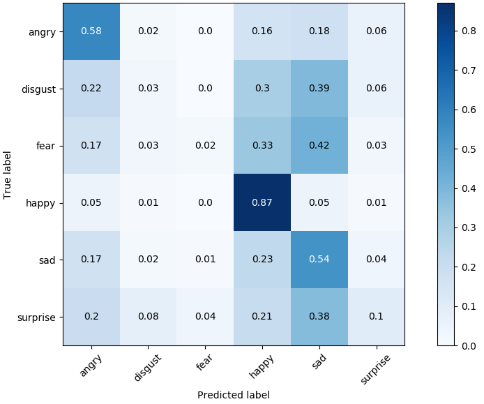
Based on this best combination of features listed in Table 9, the detailed results are delineated in Table 10. Again, we may obtain a clear insight into the model’s prediction or misclassification from the confusion matrix illustrated in Fig. 3.

Labels	Precision	Recall	F1(micro)
angry	0.547	0.585	0.565
disgust	0.136	0.030	0.049
fear	0.143	0.017	0.030
happy	0.645	0.873	0.742
sad	0.425	0.535	0.473
surprise	0.205	0.100	0.134
Average	0.454	0.530	0.476

Table 10: Detailed Results of Best Model with Unigram and Tf-idf as Features

Figure 3: Confusion Matrix (Accuracy) for Best SVM model with unigram and tf-idf as features

6 Discussion and Conclusions

The linguistic motivation behind this project was inspired by the growing field of computational research in natural languages, particularly in the Bangla language processing because Bangla is one of the most widely spoken languages; it ranked 7th in the world, with staggering number of 268 million native speakers. However, the computational motivation was to compare the contribution of different features on the performance of a classifier in doing fine-grained Bangla emotion analysis. The findings of this study imply that the SVM model that best predicted the aforementioned emotions in Bangla text composed of social-media comments, was a model that used a non-linear RBF-kernel, which yielded an accuracy of 52.98% and an F1-score of 0.3324 (macro) and 0.476 (micro). These scores showed a significant improvement over the Baseline model, with nearly a 20.08% increase in accuracy. Additionally, both the F1 macro and micro scores increased by 0.217 and 0.284, respectively.

References

- Dandapat et al. (2009) Sandipan Dandapat, Priyanka Biswas, Monojit Choudhury, and Kalika Bali. 2009. Complex linguistic annotation—no easy way out!: a case from bangla and hindi pos labeling tasks. In Proceedings of the third linguistic annotation workshop, pages 10–18. Association for Computational Linguistics.
- Das (2011) Dipankar Das. 2011. Analysis and tracking of emotions in english and bengali texts: A computational approach. International World Wide Web Conference (IW3C2).
- Das and Bandyopadhyay (2010a) Dipankar Das and Sivaji Bandyopadhyay. 2010a. Developing bengali wordnet affect for analyzing emotion. In International Conference on the Computer Processing of Oriental Languages, pages 35–40.
- Das and Bandyopadhyay (2010b) Dipankar Das and Sivaji Bandyopadhyay. 2010b. Labeling emotion in bengali blog corpus–a fine grained tagging at sentence level. In Proceedings of the 8th Workshop on Asian Language Resources, page 47.
- Das et al. (2012) Dipankar Das, Sagnik Roy, and Sivaji Bandyopadhyay. 2012. Emotion tracking on blogs-a case study for bengali. In International Conference on Industrial, Engineering and Other Applications of Applied Intelligent Systems, pages 447–456. Springer.
- Ekman (1999) P Ekman. 1999. Basic emotions in t. dalgleish and t. power (eds.) the handbook of cognition and emotion pp. 45-60.
- Honnibal and Montani (2017) Matthew Honnibal and Ines Montani. 2017. spacy 2: Natural language understanding with bloom embeddings, convolutional neural networks and incremental parsing. To appear.
- Liew and Turtle (2016) Jasy Suet Yan Liew and Howard R Turtle. 2016. Exploring fine-grained emotion detection in tweets. In Proceedings of the NAACL Student Research Workshop, pages 73–80.
- Pedregosa et al. (2011) F. Pedregosa, G. Varoquaux, A. Gramfort, V. Michel, B. Thirion, O. Grisel, M. Blondel, P. Prettenhofer, R. Weiss, V. Dubourg, J. Vanderplas, A. Passos, D. Cournapeau, M. Brucher, M. Perrot, and E. Duchesnay. 2011. Scikit-learn: Machine Learning in Python . Journal of Machine Learning Research, 12:2825–2830.