Organic complexity in protostellar disk candidates

Abstract

We present ALMA observations of organic molecules towards five low-mass Class 0/I protostellar disk candidates in the Serpens cluster. Three sources (Ser-emb 1, Ser-emb 8, and Ser-emb 17) present emission of CH₃OH as well as CH₃OCH₃, CH₃OCHO, and CH₂CO, while NH₂CHO is detected in just Ser-emb 8 and Ser-emb 17. Detecting hot corino-type chemistry in three of five sources represents a high occurrence rate given the relative sparsity of these sources in the literature, and this suggests a possible link between protostellar disk formation and hot corino formation. For sources with CH₃OH detections, we derive column densities of 10¹⁷–10¹⁸ cm^-2 and rotational temperatures of $\sim$200–250 K. The CH₃OH-normalized column density ratios of large, oxygen-bearing COMs in the Serpens sources and other hot corinos span two orders of magnitude, demonstrating a high degree of chemical diversity at the hot corino stage. Resolved observations of a larger sample of objects are needed to understand the origins of chemical diversity in hot corinos, and the relationship between different protostellar structural elements on disk-forming scales.

1 Introduction

Planet formation takes place in the gas- and dust-rich disks orbiting young stars. The chemical inventories in these protoplanetary disks therefore influence the compositions of nascent planets. It is of particular interest to origins of life studies to understand the chemistry of complex (6+ atom, hydrogen-rich) organic molecules (COMs) in planet-forming regions, since these species are considered to be precursors for prebiotic chemistry (Herbst & van Dishoeck, 2009; Jørgensen et al., 2012).

The process of star (and eventually planet) formation begins in the dense cores of molecular clouds. The youngest protostars, termed Class 0, are still deeply embedded in their natal envelope. Class I protostars are undergoing envelope infall and accretion onto a circumstellar disk, and Class II protostars have cleared their envelope and host Keplerian disks that feed accretion onto the star (Lada, 1987; Andre et al., 1993; Dunham et al., 2014). Planet formation was historically thought to take place during the Class II stage. In recent years, the high sensitivity and spatial resolution of ALMA has enabled the characterization of complex organic molecule emission in Class II disks, enhancing our understanding of organic chemistry at this stage (Öberg et al., 2015; Walsh et al., 2016; Bergner et al., 2018; Loomis et al., 2018; Favre et al., 2018). However, there is growing evidence suggesting that planet formation begins at earlier evolutionary stages (Harsono et al., 2018). Notably, high-resolution (sub-)mm continuum observations are revealing that dust sub-structure appears ubiquitous in Class II disks (Andrews et al., 2018). One compelling explanation for this sub-structure is interactions of large (Neptune- to Jupiter-mass) planets with the disk (Zhang et al., 2018), which would require that the planet formation process begins in younger (Class 0/I) disks. This scenario is supported by observations of sub-structure in the embedded disk HL Tau (ALMA Partnership et al., 2015), implying grain growth or even planet formation at an early evolutionary stage.

Some deeply embedded protostars are seen to host a rich and warm gas-phase organic chemistry on small ($\sim$100 AU) scales. These sources, termed hot corinos, form when temperatures around the protostar exceed the water ice sublimation point, and ice mantles are liberated into the gas phase (Herbst & van Dishoeck, 2009). At present, the physical nature of hot corinos is unknown because they are generally unresolved or marginally resolved in observations. Several structural elements, including protostellar disks, centrifugal barriers, and outflows, occur on similar spatial scales within the protostellar inner envelope (Sakai et al., 2014; Lee et al., 2014; Harsono et al., 2014; Yen et al., 2015); without high-sensitivity and high-resolution observations it is difficult to disentangle if these elements are related or distinct in their physics and chemistry, and which, if any, are sources of hot corino chemistry.

Since protostellar disks are likely the sites where planet formation begins, it is of great interest to understand whether the organic complexity detected in hot corinos is related to the material incorporated into the disk. To date there is no conclusive tie between hot corinos and protostellar disks. Some sources with hot corinos appear to show velocity structure in their molecular line emission consistent with the presence of a rotating disk (Choi et al., 2010; Lee et al., 2014; Codella et al., 2014; Oya et al., 2016, 2017). Still, other hot corino sources show no clear signatures of a rotating disk (Maury et al., 2014; Imai et al., 2016; Jacobsen et al., 2018). More observations are needed to understand the chemical and physical relationships between hot corinos and protostellar disks.

In this work, we present ALMA observations of five protostellar disk candidates in the Serpens cluster. For one source, Ser-emb 1, the chemical and physical structure was studied in detail in Martin-Domenech et al. (2019). Here, we aim to characterize the complex organic chemistry in all five sources in order to further our understanding of the chemical evolution of protostars on small scales. Section 2 describes our source selection, line targets, and ALMA observations. Section 3 presents the observed morphologies for each source as well as organic molecule detections. Additionally, we derive column densities for CH₃OH using the population diagram method, and for other species by assuming a rotational temperature. In Section 4 we discuss the frequency of hot corino detection in our sample of disk candidates. We also compare the CH₃OH-normalized column density ratios of organics in the Serpens sources with measurements in other hot corinos, low-mass protostellar envelopes, and Solar System comets.

2 Observations

2.1 Observational details

The source sample consists of five low-mass protostars in the Serpens cluster. Each target source shows non-zero flux at $>$50k$\lambda$ $uv$ distances measured for the 230 GHz continuum, which may be due to the presence of a protostellar disk (Enoch et al., 2011). Source properties and candidate disk mass estimates are listed in Table 1. For all sources we assume a distance of 436 $\pm$ 9 pc (Ortiz-León et al., 2018).

Source	R.A.	Decl.	Class	$T_{bol}$	$L_{bol}$	$M_{env}$	Est. $M_{disk}$ a
	(J2000)	(J2000)		(K)	($L_{\odot}$)	($M_{\odot}$)	($M_{\odot}$)
Ser-emb 1	18:29:09.1	0:31:30.9	0	39 [2]	4.1 [0.3]	3.1 [0.05]	0.28
Ser-emb 7	18:28:54.1	0:29:30.0	0	58 [13]	7.9 [0.3]	4.3 [0.4]	0.15
Ser-emb 8	18:29:48.1	1:16:43.7	0	58 [16]	5.4b [6.2]	9.4 [0.3]	0.25
Ser-emb 15	18:29:54.3	0:36:00.8	I	101 [43]	0.4 [0.6]	1.3 [0.1]	0.15
Ser-emb 17	18:29:06.2	0:30:43.1	I	117 [21]	3.8 [3.3]	3.6 [0.4]	0.15

Table 1: Source properties, taken from Enoch et al. (2009) and Enoch et al. (2011). ^aUncertainties are at least $\pm$50%. ^bLikely an underestimate.

The targets were observed during ALMA Cycle 3 from May to June of 2016, as part of project 2015.1.00964.S (PI: K. Öberg). Observations were taken in two different Band 6 spectral setups ranging from 217 – 233 GHz and 243 – 262 GHz. For the lower-frequency setup, each source was observed for $\sim$18 total minutes in two execution blocks, with 42 antennae and baselines spanning 15 – 560 m. J1751+0939 was used for bandpass and flux calibration, Titan for flux calibration, and J1830-0619 for phase calibration. For the higher-frequency setup, each source was observed for $\sim$21 total minutes in three execution blocks, with 41 antennae and baselines spanning 15 – 640 m. J1751+0939 was used for bandpass calibration, Titan for flux calibration, and J1830+0619 for phase calibration. This project makes use of data from three spectral windows centered on 219.57 GHz, 231.49 GHz, and 244.88 GHz. The 219 GHz window has a bandwidth of 117 MHz and a channel width of 122 kHz ($\sim$0.16 km/s), and the 231 and 244 GHz windows each have a bandwidth of 1.875 GHz and channel width of 488 kHz ($\sim$0.6 km/s).

Spectral window	Beam dim.	Beam	Chan. width	Chan. rms
center frequency	(”)	PA (o)	(km s-1)	(mJy beam-1)
Ser-emb 1
219 GHz	0.63 $\times$ 0.50	-68.5	0.25	5.2
231 GHz	0.57 $\times$ 0.45	-62.5	0.63	1.9
244 GHz	0.54 $\times$ 0.45	-59.7	0.60	2.3
Ser-emb 7
219 GHz	0.61 $\times$ 0.50	-69.5	0.25	5.3
231 GHz	0.57 $\times$ 0.45	-61.8	0.63	2.0
244 GHz	0.53 $\times$ 0.45	-59.9	0.60	2.2
Ser-emb 8
219 GHz	0.63 $\times$ 0.51	-66.8	0.25	5.7
231 GHz	0.57 $\times$ 0.45	-60.9	0.63	2.0
244 GHz	0.55 $\times$ 0.46	-63.5	0.60	2.2
Ser-emb 15
219 GHz	0.67 $\times$ 0.50	-65.7	0.25	5.4
231 GHz	0.58 $\times$ 0.45	-62.2	0.63	1.9
244 GHz	0.54 $\times$ 0.45	-59.0	0.60	2.2
Ser-emb 17
219 GHz	0.63 $\times$ 0.48	-64.6	0.25	5.3
231 GHz	0.57 $\times$ 0.45	-61.7	0.63	1.9
244 GHz	0.54 $\times$ 0.45	-58.1	0.60	2.2

Table 2: Line observation details

2.2 Analysis

Initial pipeline calibration of the ALMA data was performed by ALMA/NAASC staff with CASA versions 4.5.3 (lower-frequency setup) and 4.7.0 (higher-frequency setup). An additional 1–2 rounds of phase self-calibration were performed for each spectral window using the line-free continuum, followed by continuum subtraction.

In addition to the C¹⁸O 2–1 line in the 219 GHz spectral window, we searched for spectral lines of organic molecules commonly detected in protostars within the 231 GHz and 244 GHz spectral windows. Spectral line parameters are taken from the JPL (PICKETT et al., 1998) and CDMS (Müller et al., 2001, 2005) catalogs. For CH₃OH we searched for lines satisfying A_ul $>$10^-5 s^-1 and upper energies $<$700 K, and for other COMs we initially searched for lines with A_ul $>$10^-4 s^-1 and upper energies $<$300 K. When generating synthetic spectra (Section 3) we include all lines with A_ul $>$10^-5 s^-1 and upper energies $<$700 K for all COMs.

Image cubes were generated using the tclean task in CASA version 5.4.1, using Briggs weighting with a robust parameter of 0.5. C¹⁸O was imaged with a velocity resolution of 0.25 km s^-1, and all organic lines were imaged at the native spectral resolution. Clean masks were drawn by hand for detected lines, and for non-detected lines the 10$\sigma$ continuum contour was used. In addition to hand-masking individual lines, we also cleaned the full data cubes using the automasking task auto-multithresh in tclean. We used the standard automasking parameters for short baseline 12m line data (sidelobethreshold = 2.0, noisethreshold = 4.5, minbeamfrac = 0.3, negativethreshold = 15.0, lownoisethreshold = 1.5). We have verified the automasking results by comparing the CH₃OH spectra extracted from the auto-masked and hand-masked images, and find they are consistent. Table 2 shows representative line observation details for each spectral window used in this work.

Molecule	Transition	Frequency	log(Aul)	$g_{u}$	$E_{u}$	$Q(T)$		Refs.
		(GHz)	(s-1)		(K)	150 K	250 K
C18Oa	2 – 1	219.560	-6.22	5	15.8	57	95	1
CH3OHb	51,4 – 41,3 A	243.916	-4.22	44	49.7	9750	26335	2
	102,8 – 93,7 A	232.419	-4.73	84	165.4
	103,7 – 112,9 E	232.946	-4.67	84	190.4
	9-1,9 – 8-0,8 E, $v_{t}$ = 1	244.338	-4.39	76	395.6
	183,16 – 174,13 A	232.783	-4.66	148	446.5
	186,13 – 195,14 &	243.397	-4.70	296	590.3
	186,12 – 195,15 A c
	223,19 – 222,20 A	244.330	-4.09	180	636.8
	233,20 – 232,21 A	243.413	-4.09	188	690.1
CH3OCH3b	130,13 – 121,12 AA & EE c	231.988	-4.04	972	80.9	221973	716914	3,4
	235,18 – 234,19 AA & EE c	243.739	-4.10	1692	287.0
CH3OCHOa	194,15 – 184,15 A	233.227	-3.74	78	123.2	59073 [1.20]d	147269 [1.97]d	5–9
	204,17 – 194,16 E	244.580	-3.68	82	135.0
NH2CHOb	112,10 – 102,9	232.274	-2.58	23	78.9	3441	7461	10
	121,12 – 111,11	243.521	-2.50	25	79.2
CH2COb	121,11 – 111,10	244.712	-3.79	75	89.4	3658	7933	11,12

Table 3: Spectral line data. ^aFrom the JPL catalogue. ^bFrom the CDMS catalogue. ^cBlended transitions. ^dNumbers in brackets represent the vibrational correction factor to the $v_{T}$ = 0,1 partition function at each temperature. References: [1] Winnewisser et al. (1985) [2] Xu et al. (2008) [3] Endres et al. (2009) [4] Groner et al. (1998) [5] Ilyushin et al. (2009) [6] Plummer et al. (1984) [7] Oesterling et al. (1999) [8] Maeda et al. (2008) [9] Favre et al. (2014) [10] Kryvda et al. (2009) [11] Brown et al. (1990) [12] Guarnieri & Huckaufa (2003)

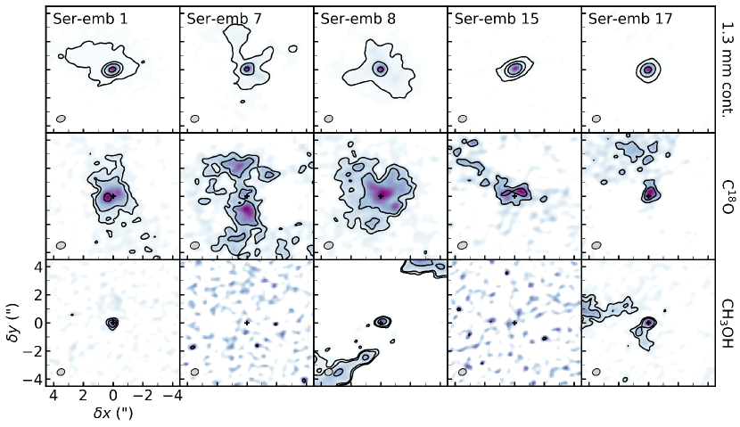
Figure 1: Source overview showing the 1.3 mm dust continuum emission (top), C¹⁸O 2–1 line emission (middle), and CH₃OH 5_1,4 – 4_1,3 line emission (bottom). Continuum contours are drawn at 5, 30, 100, 400$\times$rms, and line contours are drawn at 5, 10, 30$\times$rms. Color scales are normalized to each individual image, and emission below a 2$\times$rms threshold is not shown. The synthesized beam is shown in the bottom left of each panel. Velocity ranges and rms values for each panel can be found in Appendix A.

3 Results

3.1 Source overview

Figure 1 shows the 1.3 mm dust continuum emission, as well as C¹⁸O 2–1 and CH₃OH 5_1,4 – 4_1,3 line emission (see Table 3 for spectral line parameters). All sources show a compact central dust component, while Ser-emb 1, Ser-emb 7, and Ser-emb 8 additionally have a more extended component. The C¹⁸O morphologies show a similar pattern, with more extended gas emission in Ser-emb 1, Ser-emb 7, and Ser-emb 8. The sources with extended continuum and C¹⁸O emission are also the least evolved, and it is not surprising that we detect a greater envelope contribution in these sources.

The CH₃OH 5_1,4 – 4_1,3 line ($E_{u}$ = 50 K) is detected above a 5$\sigma$ level only towards Ser-emb 1, Ser-emb 8, and Ser-emb 17. Interestingly, the morphology of this transition is different in each source: while all three have a compact central component, Ser-emb 8 also shows a jet-like feature extending out from the central protostar, and Ser-emb 17 shows more amorphous extended emission. This extended emission is only seen for the 50 K CH₃OH line, and all higher-J lines show emission only from the compact central component (Figure 2).

Our source sample spans a relatively wide range of bolometric temperatures, bolometric luminosities, envelope masses, and estimated disk masses, however there is no clear relationship between these physical properties and the detection of CH₃OH in a source (Table 1). For each property, the value of one or both sources with CH₃OH non-detections falls within the range of values for sources with detections. We note that there are high uncertainties on the source luminosities for Ser-emb 8 and 17 and on the candidate disk masses for all sources, so better constraints on these properties may reveal some trend with CH₃OH emission. There is also no clear relationship between the inferred size of the disk and the presence of CH₃OH emission: in the observations of Enoch et al. (2011), the mm dust emission is compact and unresolved at spatial scales of $\sim$170 AU in Ser-emb 7, Ser-emb 15, and Ser-emb 17, but partially resolved in Ser-emb 1 and Ser-emb 8. The protostellar neighborhood also does not appear to account for CH₃OH emission: none of the sources show evidence for binarity in the Enoch et al. (2011) survey, and Ser-emb 1 is the only source that is isolated more than $\sim$30” from one or two neighboring protostars. Moreover, Ser-emb 1, 7, and 17 are located near to one another in the Serpens cluster B, while Ser-emb 15 is farther away in cluster B and Ser-emb 8 is in the Main cluster (Enoch et al., 2011). The presence of CH₃OH emission might be influenced by a combination of these and other factors, however, and better characterization of the physical properties of each source as well as their local physical environment is needed.

3.2 Organic molecule detections

The sources with CH₃OH detections (Ser-emb 1, Ser-emb 8, and Ser-emb 17) also showed emission from other organic molecules. We consider a molecule to be detected based on the following criteria. At least one line must be observed above a 5$\sigma$ level in the moment zero map, and the peak of the extracted spectrum must similarly be $>$5$\sigma$. For each line, we also check for possible neighbors and do not further consider any lines that are potentially blended with other strong emitters. Lastly, we search the spectra for other lines of each detected molecule to ensure that any strong transitions are not missing. Based on these criteria, CH₃OCH₃, CH₃OCHO, and CH₂CO were detected towards Ser-emb 1, Ser-emb 8, and Ser-emb 17, while NH₂CHO was detected just towards Ser-emb 8 and Ser-emb 17. We note that the CH₂CO detections are based on a single line, however because it is unblended and there are no competing line assignments we are confident in the detection. Figure 2 shows moment zero maps for the brightest transition of each of these organic molecules, along with a high-energy ($E_{u}$ = 165 K) CH₃OH line. In all cases, the emission is unresolved or marginally resolved.

In several sources we also see evidence for emission from HCOOH, CH₃CHO, C₂H₅OH, and possibly CH₂OHCHO. However, there are too few lines that are both unblended and have sufficient SNR to claim detections. Higher resolution data and an increased number of line targets per molecule are needed to characterize the emission from these additional species.

Table 3 lists the spectral line information for the transitions that we use for measuring column densities. Additional CH₃OCHO lines are covered in the frequency range of our spectra, however due to line overlap we consider only these non-blended lines for analysis. We note that the CH₃OCHO partition function from JPL includes the $v_{T}$= 0,1 states, however at hot corino temperatures (200–300 K) other vibrational states will become populated. We therefore correct the partition function with the vibrational correction factors provided by Favre et al. (2014) via the CMDS catalogue; Table 3 lists the non-corrected partition function values and vibrational correction factors at each temperature. For other molecules, the catalogs already include sufficient vibrationally excited states in the partition function or the vibrational contributions are small at hot corino temperatures; the exception is NH₂CHO for which the vibrational contribution is not yet available.

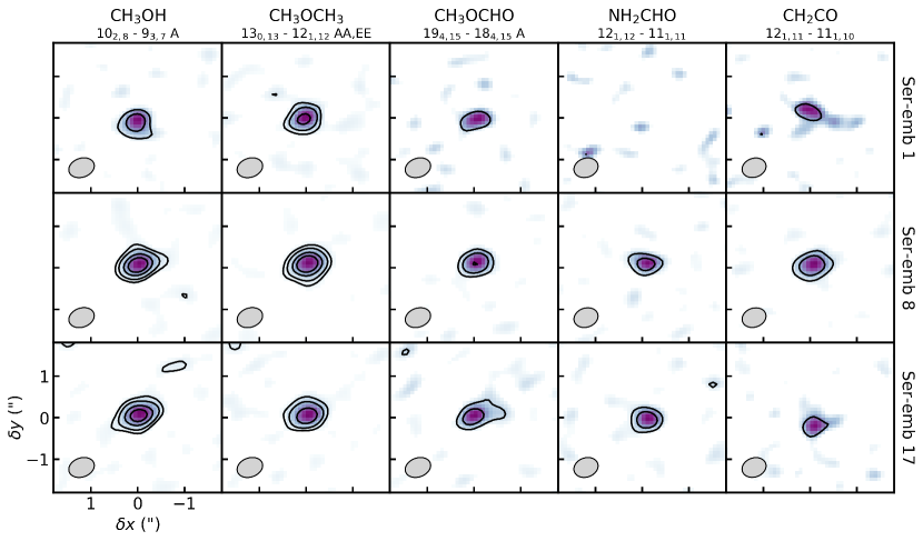
Figure 2: Moment zero maps of organic molecule lines in Ser-emb 1, Ser-emb 8, and Ser-emb 17. Contours are drawn at 5, 10, 20, 30$\times$rms. Color scales are normalized to each individual image, and emission below a 2$\times$rms threshold is not shown. The synthesized beam is shown in the bottom left of each panel. Velocity ranges and rms values for each panel can be found in Appendix A.

3.3 Column densities

3.3.1 CH₃OH

For each source, we extract spectra from a single pixel corresponding to the location of the continuum peak. Velocity-integrated intensities are measured by fitting a Gaussian to each spectral feature. For isolated lines we also include an offset term in the fit to allow slight variations in the baseline. For each source, the line width derived for the CH₃OH 5_1,4 – 4_1,3 transition is adopted as a fixed parameter for all other transitions to ensure good fits for weaker or slightly blended lines. All CH₃OH spectral lines and Gaussian fits are shown in Figure 3. Integrated intensities can be found in Table 5. Subsequent uncertainties are propagated based on Gaussian fit uncertainties added in quadrature with a 10% calibration uncertainty.

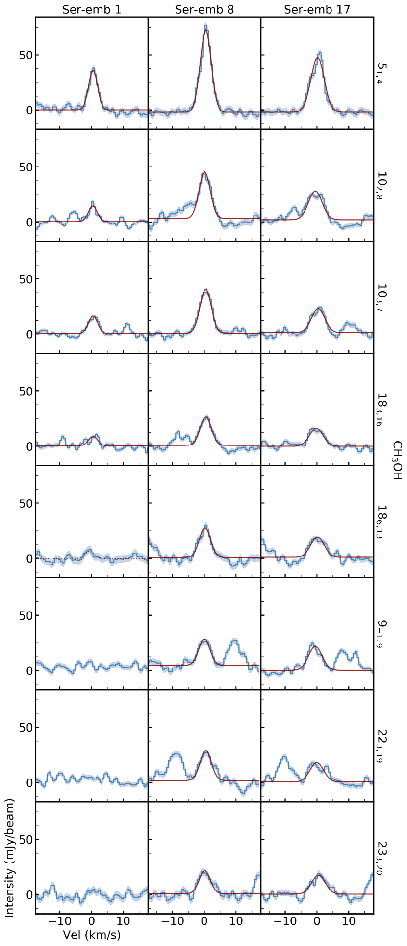
Figure 3: CH₃OH spectral lines in sources where CH₃OH is detected. Blue lines show the spectra extracted from the continuum peak pixel, and shaded regions represent the rms. Red lines show Gaussian fits to the data; a dotted line indicates that the feature is not significant above a 3$\sigma$ level.

Our observations cover 8 CH₃OH transitions spanning a range of upper state energies from 50 – 690 K. We use the population diagram method to derive column densities and rotational temperatures, taking into account optical depths for each line. This treatment is adapted from Goldsmith & Langer (1999) (see also e.g. Taquet et al. (2015); Loomis et al. (2018)) and assumes local thermodynamic equilibrium (LTE) conditions.

The total column density $N_{T}$ and rotational temperature $T_{R}$ are related to the upper level population $N_{u}$ by:

$$\frac{N_{u}}{g_{u}}=\frac{N_{T}}{Q(T_{R})}e^{-E_{u}/T_{R}}$$ (1)

Here, $g_{u}$ is the upper level degeneracy, $Q$ is the molecular partition function, and $E_{u}$ is the upper state energy in K. The observed upper level population $N_{u,obs}$ is found from the velocity-integrated surface brightness $\int I_{\nu}dv$ by:

$$N_{u,obs}=\frac{4\pi\int I_{\nu}dv}{A_{ul}hc},$$ (2)

where $A_{ul}$ is the transition Einstein coefficient. If the source does not fill the beam and if the observed lines are optically thick, we find the true upper level population from $N_{u,obs}$ by:

$$N_{u}=N_{u,obs}C_{\tau}\frac{\Omega_{a}}{\Omega_{s}}.$$ (3)

$C_{\tau}$ is the optical depth correction factor and $\frac{\Omega_{a}}{\Omega_{s}}$ is the beam dilution factor, where $\Omega_{s}$ and $\Omega_{a}$ are the source and beam solid angles, respectively. $C_{\tau}$ is found from:

$$C_{\tau}=\frac{\tau}{1-e^{-\tau}},$$ (4)

and the optical depth $\tau$ is determined by:

$$\tau=\frac{c^{3}A_{ul}N_{u}}{8\pi\nu^{3}\Delta v}(e^{h\nu/kT_{R}}-1).$$ (5)

Here, $c$ is the speed of light, $A_{ul}$ is the Einstein coefficient (lines with a higher $A_{ul}$ are more likely to be optically thick), $\nu$ is the line frequency, $\Delta v$ is the line full width half-maximum, and $k$ is the Boltzmann constant. For $\Delta v$ we use the FWHM of the CH₃OH 5_1,4–4_1,3 line in each source (3.3, 4.0, and 4.9 km/s in Ser-emb 1, 8, and 17, respectively).

The degree of beam dilution in our observations is uncertain given that the sources are unresolved or barely resolved. We therefore solve for column densities using two bounding cases to represent the range of likely values. The maximum source size, corresponding to the minimum beam dilution, is found using the deconvolved source sizes (or upper limits) derived in CASA for the CH₃OH 165 K or 190 K lines (since the 50 K line traces cooler material in addition to the hot corino). This gives beam dilution factors of 8.7, 15.1, and 9.3 for Ser-emb 1, 8, and 17, respectively. The minimum source size, corresponding to the maximum beam dilution, is found by using the power-law temperature profile for protostellar envelopes in Chandler & Richer (2000) to estimate the radius beyond which the temperature falls below 100 K:

$$T(r)=60\Bigg{(}\frac{r}{2\times 10^{15}\rm{m}}\Bigg{)}^{-q}\Bigg{(}\frac{L_{\rm{bol}}}{10^{5}L_{\odot}}\Bigg{)}^{q/2}\rm{K},$$ (6)

where $q$ = 2/(4 + $\beta$). Assuming the source luminosities in Table 1 and $\beta$ = 1.5, we find maximum beam dilution factors of 27.7, 21.0, and 29.7 for Ser-emb 1, 8, and 17, respectively.

We fit the observed upper level populations (Equation 2) by generating synthetic upper level populations for all detected CH₃OH transitions, with $N_{T}$ and $T_{R}$ as free parameters. Combining Equations 1 and 3, the synthetic $N_{u,obs}$ are found from:

$$\frac{N_{u,obs}}{g_{u}}=\frac{N_{T}}{Q(T_{R})}e^{-E_{u}/T_{R}}\frac{1}{C_{\tau}}\frac{\Omega_{s}}{\Omega_{a}}.$$ (7)

We use the affine-invariant MCMC package emcee (Foreman-Mackey et al., 2013) to sample the posterior distributions. Additional details on the MCMC fitting can be found in Appendix B. All spectral line parameters used for this analysis are listed in Table 3.

The resulting population diagrams are shown in Figure 4. Table 4 lists the values derived from this fitting, along with 1$\sigma$ uncertainties. Across the sample, we derive column densities on the order of 10¹⁷ cm^-2 and rotational temperatures of 200–250 K. Even in the maximum beam dilution cases, in all sources the optical depth of the 50 K line is $<$0.9 and the optical depths of all other lines are $<$0.4.

In hot corino sources where CH₃OH lines are optically thick, ¹³CH₃OH or CH${}_{3}^{18}$OH lines are often used to derive CH₃OH column densities (Taquet et al., 2015; Jørgensen et al., 2016). Our observations cover the ¹³CH₃OH line at 231.818 GHz, however we do not detect this line in any source. Assuming the maximum beam dilution factor, and a ¹²C/¹³C ratio of 70, we obtain 3$\sigma$ upper limits on the CH₃OH column density of a few $\times$10¹⁹ cm^-2 for our sources. Thus, these non-detections are consistent with our derived column densities but do not provide any further constraints.

	Min. $\frac{\Omega_{a}}{\Omega_{s}}$		Max. $\frac{\Omega_{a}}{\Omega_{s}}$
	NT (1017 cm-2)	TR (K)	NT (1017 cm-2)	TR (K)
Ser-emb 1	1.4 ${}_{-0.2}^{+0.2}$	256 ${}_{-28}^{+32}$	4.5 ${}_{-0.7}^{+0.6}$	256 ${}_{-28}^{+32}$
Ser-emb 8	5.7 ${}_{-0.3}^{+0.3}$	213 ${}_{-8}^{+8}$	8.0 ${}_{-0.4}^{+0.4}$	213 ${}_{-8}^{+8}$
Ser-emb 17	2.8 ${}_{-0.1}^{+0.1}$	224 ${}_{-9}^{+10}$	9.0 ${}_{-0.5}^{+0.5}$	224 ${}_{-9}^{+9}$

Table 4: CH₃OH column densities and rotational temperatures and 1$\sigma$ uncertainties derived from population diagram fitting, assuming minimum and maximum beam dilution factors as described in the text.

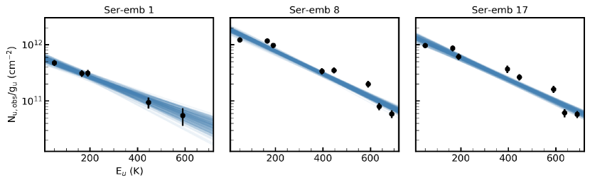
Figure 4: CH₃OH population diagrams for Ser-emb 1, Ser-emb 8, and Ser-emb 17. Data and uncertainties are shown in black, and draws from the fit posteriors are shown in blue.

3.3.2 Other organics

For all additional organics, detected lines are fitted with Gaussians as described previously for CH₃OH. Again, we adopt the line width of the CH₃OH 5_1,4 – 4_1,3 transition for all other molecular lines observed towards a given source. Spectral line fits for all detected lines can be found in Appendix C, and integrated intensities are listed in Table 5.

Molecule	Line	Ser-emb 1		Ser-emb 8		Ser-emb 17
		Int. intensity	Beam dim.	Int. intensity	Beam dim.	Int. intensity	Beam dim.
		(mJy beam-1	(”)	(mJy beam-1	(”)	(mJy beam-1	(”)
		km s-1)		km s-1)		km s-1)
CH3OH	51,4	127 $\pm$ 15	0.54 $\times$ 0.45	325 $\pm$ 34	0.55 $\times$ 0.46	262 $\pm$ 29	0.54 $\times$ 0.45
	102,8	49 $\pm$ 7	0.57 $\times$ 0.45	187 $\pm$ 21	0.57 $\times$ 0.45	139 $\pm$ 16	0.57 $\times$ 0.45
	103,7	57 $\pm$ 8	0.57 $\times$ 0.45	178 $\pm$ 19	0.57 $\times$ 0.45	113 $\pm$ 15	0.57 $\times$ 0.45
	183,16	31 $\pm$ 7	0.57 $\times$ 0.45	114 $\pm$ 14	0.57 $\times$ 0.45	88 $\pm$ 12	0.57 $\times$ 0.45
	186,13	33 $\pm$ 12	0.54 $\times$ 0.45	120 $\pm$ 16	0.54 $\times$ 0.45	98 $\pm$ 14	0.54 $\times$ 0.45
	9-1,9	-	-	106 $\pm$ 14	0.53 $\times$ 0.45	117 $\pm$ 18	0.54 $\times$ 0.45
	223,19	-	-	120 $\pm$ 18	0.53 $\times$ 0.45	93 $\pm$ 16	0.54 $\times$ 0.45
	233,20	-	-	92 $\pm$ 15	0.54 $\times$ 0.45	92 $\pm$ 13	0.54 $\times$ 0.45
CH3OCH3	130,13	102 $\pm$ 12	0.57 $\times$ 0.45	234 $\pm$ 25	0.57 $\times$ 0.45	135 $\pm$ 16	0.57 $\times$ 0.45
	235,18	74 $\pm$ 10	0.54 $\times$ 0.45	74 $\pm$ 11	0.55 $\times$ 0.46	93 $\pm$ 13	0.54 $\times$ 0.45
CH3OCHO	194,15	35 $\pm$ 10	0.57 $\times$ 0.45	89 $\pm$ 12	0.57 $\times$ 0.45	67 $\pm$ 12	0.57 $\times$ 0.45
	204,17	48 $\pm$ 9	0.53 $\times$ 0.45	118 $\pm$ 14	0.55 $\times$ 0.46	90 $\pm$ 14	0.54 $\times$ 0.45
NH2CHO	112,10	-	-	51 $\pm$ 8	0.57 $\times$ 0.45	44 $\pm$ 11	0.57 $\times$ 0.45
	121,12	-	-	64 $\pm$ 10	0.54 $\times$ 0.45	68 $\pm$ 11	0.54 $\times$ 0.45
CH2CO	121,11	30 $\pm$ 7	0.53 $\times$ 0.45	101 $\pm$ 13	0.53 $\times$ 0.45	42 $\pm$ 10	0.54 $\times$ 0.45

Table 5: Integrated intensities and uncertainties for spectra extracted from the continuum peak pixel. For clarity, only upper state quantum numbers are used to identify each line; refer to Table 3 for full identifiers.

We estimate column densities by solving equations 2 and 7 assuming optically thin emission and an adopted rotational temperature. We expect most COMs to share a roughly similar rotational temperature as CH₃OH, though some species tend to emit at cooler or warmer temperatures (Jørgensen et al., 2016). We therefore calculate column densities assuming the CH₃OH rotational temperatures derived in the previous section ($T_{M}$), as well as $T_{M}$ $\pm$ 75 K. As for CH₃OH, we calculate the range of column density values assuming minimum and maximum beam dilution factors. The results are listed in Table 6.

Figure 5 shows the complete spectrum extracted from Ser-emb 17 along with synthetic spectra for each organic molecule, calculated with the derived column densities and assuming the CH₃OH rotational temperature. Spectra for all additional sources can be found in Appendix D. Synthetic spectra are calculated for all lines with A_ul $>$10^-5 s^-1 and upper energies $<$700 K. The optical depths calculated for all COM lines are low ($<$0.3), confirming our assumption of optically thin emission.

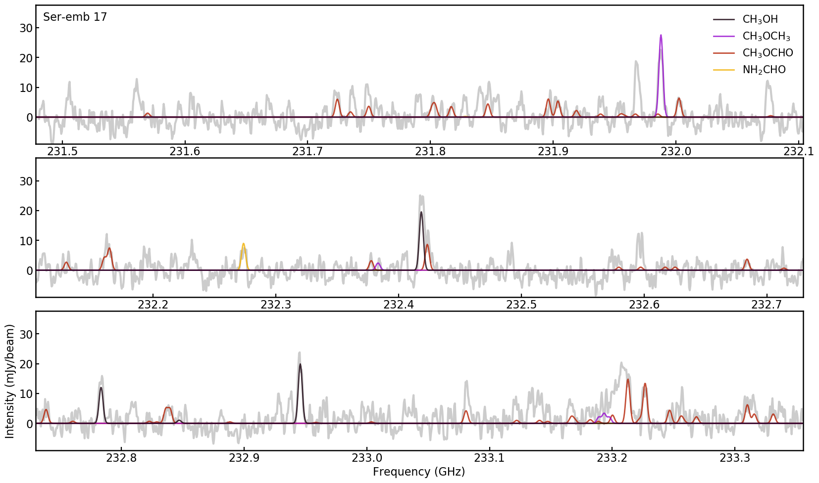
(a)

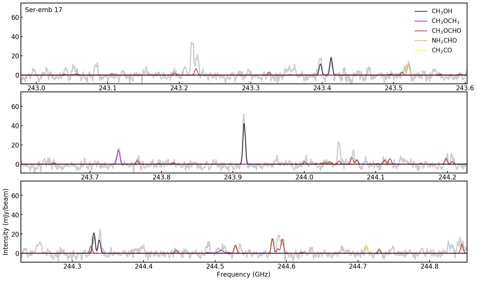
(b)

Figure 5: Full spectrum extracted from the continuum peak pixel in Ser-emb 17 (grey line), along with synthetic spectra of the COMs studied in this work (colored lines) assuming the CH₃OH rotational temperature.

	CH3OCH3		CH3OCHO		NH2CHO		CH2CO
	NT (1017 cm-2)		NT (1017 cm-2)		NT (1015 cm-2)		NT (1015 cm-2)
	Min. $\frac{\Omega_{a}}{\Omega_{s}}$	Max. $\frac{\Omega_{a}}{\Omega_{s}}$	Min. $\frac{\Omega_{a}}{\Omega_{s}}$	Max. $\frac{\Omega_{a}}{\Omega_{s}}$	Min. $\frac{\Omega_{a}}{\Omega_{s}}$	Max. $\frac{\Omega_{a}}{\Omega_{s}}$	Min. $\frac{\Omega_{a}}{\Omega_{s}}$	Max. $\frac{\Omega_{a}}{\Omega_{s}}$
Ser-emb 1	1.1 ${}_{0.7}^{1.2}$	3.4 ${}_{2.2}^{4.0}$	1.2 ${}_{0.5}^{1.7}$	3.7 ${}_{1.7}^{5.3}$	-	-	2.5 ${}_{1.7}^{2.9}$	7.9 ${}_{5.5}^{9.2}$
Ser-emb 8	2.2 ${}_{1.3}^{3.6}$	3.0 ${}_{1.8}^{5.0}$	3.1 ${}_{1.5}^{6.5}$	4.3 ${}_{2.0}^{9.0}$	3.1 ${}_{2.0}^{4.4}$	4.3 ${}_{2.8}^{6.2}$	11.8 ${}_{7.8}^{16.6}$	16.4 ${}_{10.8}^{23.0}$
Ser-emb 17	1.2 ${}_{0.8}^{1.8}$	3.7 ${}_{2.4}^{5.7}$	1.7 ${}_{0.8}^{3.5}$	5.3 ${}_{2.4}^{11.1}$	1.9 ${}_{1.2}^{2.7}$	6.1 ${}_{3.9}^{8.6}$	3.1 ${}_{2.1}^{4.3}$	9.9 ${}_{6.5}^{13.8}$

Table 6: Organic molecule column density estimates. Column densities are calculated assuming two bounding beam dilution factors, as described in the text. For each beam dilution factor, column densities are shown for three rotational temperature assumptions: $T_{M}$ ${}_{-75K}^{+75K}$, where $T_{M}$ is the CH₃OH rotational temperature derived in each source. When multiple lines are detected, the listed column density is the uncertainty-weighted average of the values calculated for each line.

4 Discussion

4.1 Frequency of hot corino chemistry around protostellar disk candidates

In our survey of five protostellar disk candidates, we see evidence for warm, organic-rich, hot-corino-like emission from three of five targeted sources. This is a high occurrence rate given that only 9 hot corinos have been previously identified in the literature: IRAS 16293-2422 (Cazaux et al., 2003), NGC1333 IRAS 4A (Bottinelli et al., 2004), NGC1333 IRAS 2 (Jørgensen et al., 2005), NGC1333 IRAS 4B (Bottinelli et al., 2007), HH 212 (Codella et al., 2016), B335 (Imai et al., 2016), L483 (Oya et al., 2017), B1b (Lefloch et al., 2018), and SVS 13-A (Lefloch et al., 2018). Our sources were selected due to their classification as protostellar disk candidates, suggesting that hot corinos and protostellar disks may be evolutionarily or structurally linked. We emphasize, however, that higher-resolution kinematic studies are needed to verify if these sources indeed host disks. Interestingly, Ser-emb 17 is just the second Class I source with a hot corino detection (Codella et al., 2016; Lefloch et al., 2018); while Class 0 sources represent the majority of hot corino detections, they are clearly not limited to this early evolutionary stage.

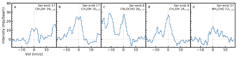
Figure 6: Examples of spectra with line profiles suggestive of rotation (a, b), infall (b, c, d), and outflows (e). For clarity, only upper state quantum numbers are used to identify each line; refer to Table 3 for full identifiers.

Given the quality of these observations, we cannot at present put strong constraints on whether the organic molecule emission we observe originates from a disk. However, we do see interesting hints of structure in the line shapes. Examples of these features are shown in Figure 6. Many organic lines in Ser-emb 17 appear to have a double-peaked line profile, which can be a signature of a rotating disk (Beckwith & Sargent, 1993) (though could also be an opacity effect). Some lines in Ser-emb 8 and Ser-emb 17 also appear to show an inverse P-cygni profile, with an absorption feature occurring at red-shifted wavelengths from the emission peak, indicative of infall (Di Francesco et al., 2001; Kristensen et al., 2012). NH₂CHO line profiles in Ser-emb 8 and 17 also show a slight broadening at red-shifted velocities, suggesting the presence of a jet/outflow. Strong NH₂CHO emission in an outflow has been previously reported towards L1157 (Codella et al., 2017). Clearly, there is evidence for additional structure in these molecular lines that is not resolved in our observations. Disentangling whether the hot corino, infall, disk, and jet/outflow components are distinct or overlapping in their chemistry and physics requires higher-resolution follow-up observations, and will be key to understanding the connection between protostellar chemistry and disk chemistry.

4.2 CH₃OH column densities

In other hot corinos that have been studied at high angular resolution (NGC1333 IRAS 2A and 4A, IRAS 16293 B, and L483)(Taquet et al., 2015; Jacobsen et al., 2018; Jørgensen et al., 2018), derived CH₃OH column densities are typically on the order 10¹⁹ cm^-2, though a lower value (a few $\times$10¹⁷ cm^-2) was found in the incipient hot corino B1b-S (Marcelino et al., 2018). The CH₃OH column densities derived in this work for the Serpens sources are $\sim$10¹⁷–10¹⁸cm^-2, consistent with B1b-S but low compared to the other hot corinos. We have accounted for beam dilution and optical depth effects as best as possible given the current observations, but additional observations are needed confirm the low CH₃OH column densities in the Serpens sources. Higher-resolution observations that cover additional CH₃OH isotopologue lines would enable more robust constraints on the degree to which beam dilution and optical depth effects impact our results.

If confirmed, the low column densities in the Serpens sources and B1b-S suggest that they are intrinsically weaker/smaller hot corinos, which could be due to their low source luminosities. This highlights the power of ALMA to detect and characterize new hot corinos that span a broad range of physical properties.

4.3 Organic abundances across evolutionary stages

It is of considerable interest to understand how the organic chemistry changes during the evolutionary progression from protostars to protoplanetary disks to planetary systems. At (sub-)millimeter wavelengths, we can directly probe the gas-phase reservoir of organics, which is also indirectly linked to the ice-phase reservoir through different desorption processes. In the cold, outer envelopes of low-mass protostars, gas-phase organic molecules likely represent the non-thermal desorption products of grain-surface chemistry. At the low densities and temperatures of these environments, the formation of saturated organics is not efficient in the gas phase and is thought to proceed exclusively in ice mantles (Horn et al., 2004; Geppert et al., 2006; Garrod & Herbst, 2006). Later, in the hot corino stage, gas-phase molecules emit from much warmer and denser regions, where most ice will have sublimated into the gas phase. Gas-phase compositions therefore reflect thermal ice desorption and possibly additional gas-phase chemistry (Herbst & van Dishoeck, 2009; Balucani et al., 2015; Skouteris et al., 2017, 2019). Finally, we can best explore COM chemistry at the Class II disk stage using cometary measurements, which are made in the gas-phase but are believed to probe pristine ices. It is not currently clear the extent to which cometary ice compositions are inherited from the interstellar medium, or reprocessed during the assembly of a planetary system. Protostellar observations suggest that material is altered by heating/shocking during infall and accretion onto the disk (Oya et al., 2016), while various lines of evidence indicate that solid material (both refractory and volatile) in outer Solar system regions is at least partially inherited (Mumma & Charnley, 2011; Altwegg et al., 2017).

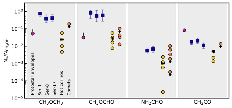
Figure 7: Comparison of organic molecule column density ratios with respect to methanol at different evolutionary stages. The Ser-emb sources are shown as blue squares. Column densities are derived for the continuum peak position, assuming the CH₃OH rotational temperature $T_{M}$; error bars show the column densities derived for $T_{M}$ $\pm$75 K. Measured abundances in the cold outer envelopes of Class 0/I low-mass protostars are shown as pink dots, hot corinos as yellow dots (+ markers indicate IRAS 16293 B), and Solar System comets as orange dots.

To explore the organic chemistry in different types of sources, we compare COM/CH₃OH column density ratios. Since CH₃OH is predicted to serve as a feedstock molecule for the formation of larger COMs in ice mantles (Öberg et al., 2009; Garrod & Herbst, 2006; Garrod et al., 2008), the COM/CH₃OH ratios can be thought of as a conversion efficiency. We also note that even in the maximum beam dilution case the optical depths of all lines are $<$1. This means that uncertainties in the beam dilution factor will cancel out when comparing COM/CH₃OH column density ratios.

Figure 7 shows the column density ratios of each organic with respect to CH₃OH in the Serpens protostellar disk candidates, along with measurements in a sample of low-mass protostellar envelopes (Bergner et al., 2017); the hot corinos IRAS 16293 B (Jørgensen et al., 2018), L483 (Jacobsen et al., 2018), NGC 1333-IRAS 2A and 4A (Taquet et al., 2015), and Barnard 1b-S (Marcelino et al., 2018) ; and the solar system comets Hale-Bopp, Lemmon, Lovejoy, and 67P summer and winter hemispheres (Bockelée-Morvan et al., 2000; Crovisier et al., 2004; Biver et al., 2014, 2015; Le Roy et al., 2015). For the Serpens sources, organic molecule column densities are calculated assuming the CH₃OH rotational temperature $T_{M}$, and error bars show the values assuming rotational temperatures of $T_{M}$ $\pm$75 K.

The NH₂CHO and CH₂CO column density ratios with respect to CH₃OH are consistent between the Serpens sources and other hot corinos, while the CH₃OCH₃ and CH₃OCHO ratios in Serpens are enhanced by at least a factor of $\sim$10 compared to the other hot corinos. There is also at least an order of magnitude spread in the CH₃OCH₃, CH₃OCHO, and NH₂CHO ratios across the other hot corinos. We note that some of this variation may be an artifact of the different angular resolutions and analysis techniques used to derive column densities. Still, at present it appears that there is a wide range in the abundances of large, oxygen-bearing molecules in different hot corino sources.

Several possible mechanisms could contribute to the observed chemical diversity in hot corinos. Given that hot corino emission is typically not well resolved, it is possible that different hot corinos host different physical components (e.g. infall, jets, accretion shocks, rotating disks) that alter what molecules are observed in the gas phase. Alternatively, chemical variation among hot corinos could reflect differences in the amounts of time spent in different physical states. For instance, the infall rate determines how long ice mantles are heated prior to sublimation, with slower infall allowing more time for the formation of larger organics in lukewarm ices (Garrod et al., 2008). Time-variable infall chemistry could also cause large differences in the observed organic inventories of different aged sources. Similarly, if gas-phase chemistry is active following ice sublimation in hot corinos, then the size and age of the hot corino should influence the observed gas-phase abundances. Interestingly, the Serpens sources are more chemically similar to one another than the other hot corinos, suggesting that the conditions in the local birth cloud may play an important role in setting the protostellar chemistry.

While some or all of these explanations could be at play, we emphasize the need for additional high-resolution and high-sensitivity observations. Expanding the number of hot corinos for which we have resolved observations of organic molecule emission will be key to understanding the variation in hot corino chemistry. Additionally, while we have modeled the CH₃OH optical depths in the Serpens sources as well as the data will allow, observations of minor CH₃OH isotopologues and/or a wider set of lines is needed to confirm the high COM to CH₃OH ratios.

As shown in Figure 7, previously studied hot corinos are chemically similar both to cold protostellar envelopes and to Solar system comets, suggestive of chemical inheritance throughout these evolutionary stages. However, the Serpens observations show that the hot corino stage is more chemically variable than previously assumed. This means that care must be taken when using protostellar observations to predict the composition of pre-cometary material in the Solar system. We need a deeper understanding of what drives chemical diversity at the hot corino stage, and in turn what sources are the best analogs to the young Sun, in order to make inferences about our chemical history.

5 Conclusions

We have surveyed the organic molecules CH₃OH, CH₃OCH₃, CH₃OCHO, NH₂CHO, and CH₂CO towards five Class 0/I protostellar disk candidates. Based on our analysis, we conclude the following:

1. Warm organic molecule emission consistent with hot corino chemistry is detected in three of five targeted sources. These observations suggest a possible association between hot corinos and protostellar disks.

2. For the three sources with CH₃OH detections, we derive column densities of 10¹⁷–10¹⁸ cm^-2 and rotational temperatures of $\sim$200–250 K. These column densities are on the low end of previously studied hot corinos, highlighting ALMA’s capacity to identify smaller or more weakly emitting hot corino sources.

3. The CH₃OH-normalized column density ratios of CH₃OCH₃ and CH₃OCHO in the Serpens sources and other hot corinos span two orders of magnitude. Local environmental effects and/or time-dependent warm-up chemistry could contribute to this chemical diversity.

4. High-resolution observations of these and other hot corino sources are required to disentangle whether hot corino emission is associated with a protostellar disk, and to better understand the origins of chemical diversity seen at the hot corino stage. This will be important for connecting Solar system comet compositions with earlier evolutionary stages.

Appendix A Moment zero map parameters

Table 7 lists the rms values and velocity ranges used to make the moment zero maps shown in Figures 1 and 2.

	Ser-emb 1		Ser-emb 7		Ser-emb 8		Ser-emb 15		Ser-emb 17
	Vel.	rms	Vel.	rms	Vel.	rms	Vel.	rms	Vel.	rms
	(km/s)	(mJy)	(km/s)	(mJy)	(km/s)	(mJy)	(km/s)	(mJy)	(km/s)	(mJy)
C18O 2	6.7–10.5	4.1	6.0–12.0	5.4	6.0–10.7	5.6	8.2–12.5	4.4	4.7–10.5	5.7
CH3OH 51,4	2.6–11.6	6.8	6.2–11.6	4.1	2.6–14.0	6.5	8.6–12.2	3.2	2.0–13.4	7.5
CH3OH 102,8	7.0–10.2	2.9	…	…	4.5–12.7	5.4	…	…	5.1–10.8	3.5
CH3OCH3 130,13	6.4–12.1	3.7	…	…	3.2–12.1	5.5	…	…	4.5–12.1	4.3
CH3OCHO 194,15	5.7–9.5	3.4	…	…	5.7–12.6	5.0	…	…	4.4–10.1	4.1
NH2CHO 121,12	6.8–9.8	3.2	…	…	6.2–12.8	5.2	…	…	5.0–12.8	5.3
CH2CO 121,11	5.6–12.1	4.7	…	…	4.4–12.1	5.4	…	…	4.4–12.1	5.1

Table 7: Velocity ranges and rms values used for the integrated intensity maps (Figures 1 and 2) in the main text. For clarity, only upper state quantum numbers are used to identify each line; refer to Table 3 for full identifiers.

Appendix B Population diagram diagram fitting

For the MCMC population diagram fits to CH₃OH, we use a flat prior 10⁵ $<$ N_T $<$ 10²⁰ cm^-2 and 100 $<$ T_r $<$ 400 K. 200 walkers are propagated for 1000 steps, and the samples are well converged. Walker chains and corner plots for each source are shown in Figures 8–10 for the maximum beam dilution case.

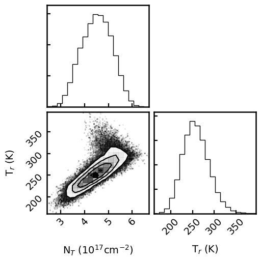
(a)

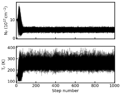
(b)

Figure 8: Ser-emb 1 rotational diagram MCMC fit results. The corner plot is shown on the left and the walker chain on the right.

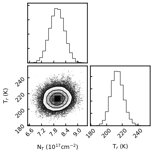
(a)

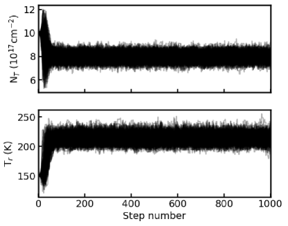
(b)

Figure 9: Ser-emb 8 rotational diagram MCMC fit results. The corner plot is shown on the left and the walker chain on the right.

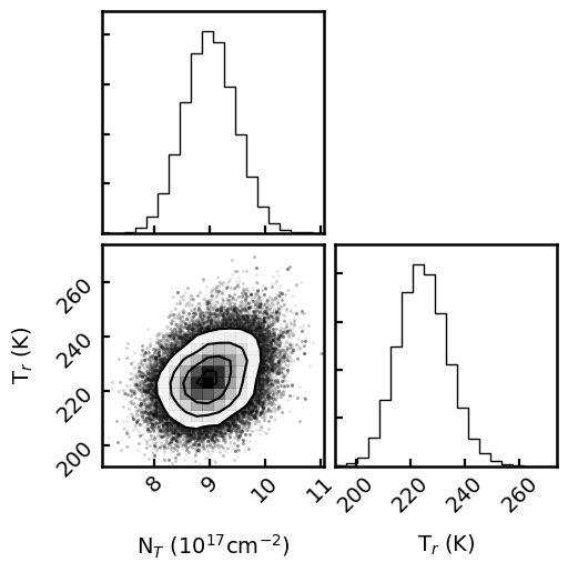
(a)

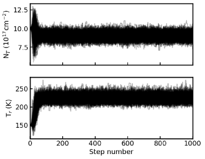
(b)

Figure 10: Ser-emb 17 rotational diagram MCMC fit results. The corner plot is shown on the left and the walker chain on the right.

Appendix C Spectral line fits

Figures 11–14 show Gaussian fits to the observed lines of each COM, analogous to Figure 3.

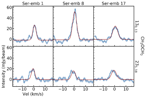
Figure 11: CH₃OCH₃ spectral lines. Blue lines show the spectra extracted from the continuum peak pixel, and shaded regions represent the rms. Red lines show Gaussian fits to the data.

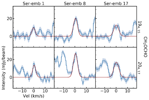
Figure 12: CH₃OCHO spectral lines. Blue lines show the spectra extracted from the continuum peak pixel, and shaded regions represent the rms. Red lines show Gaussian fits to the data.

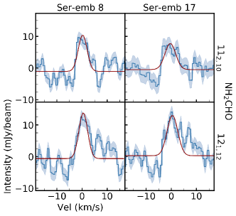
Figure 13: NH₂CHO spectral lines. Blue lines show the spectra extracted from the continuum peak pixel, and shaded regions represent the rms. Red lines show Gaussian fits to the data.

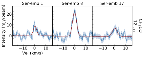
Figure 14: CH₂CO spectra lines. Blue lines show the spectra extracted from the continuum peak pixel, and shaded regions represent the rms. Red lines show Gaussian fits to the data.

Appendix D Full spectra

Figures 15–18 show the full spectra extracted from the continuum peak pixel in Ser-emb 1, 7, 8, and 15, analogous to Figure 5. For Ser-emb 1 and 8 (Figures 15 and 17) colored lines show the synthetic spectra of COMs detected in each source.

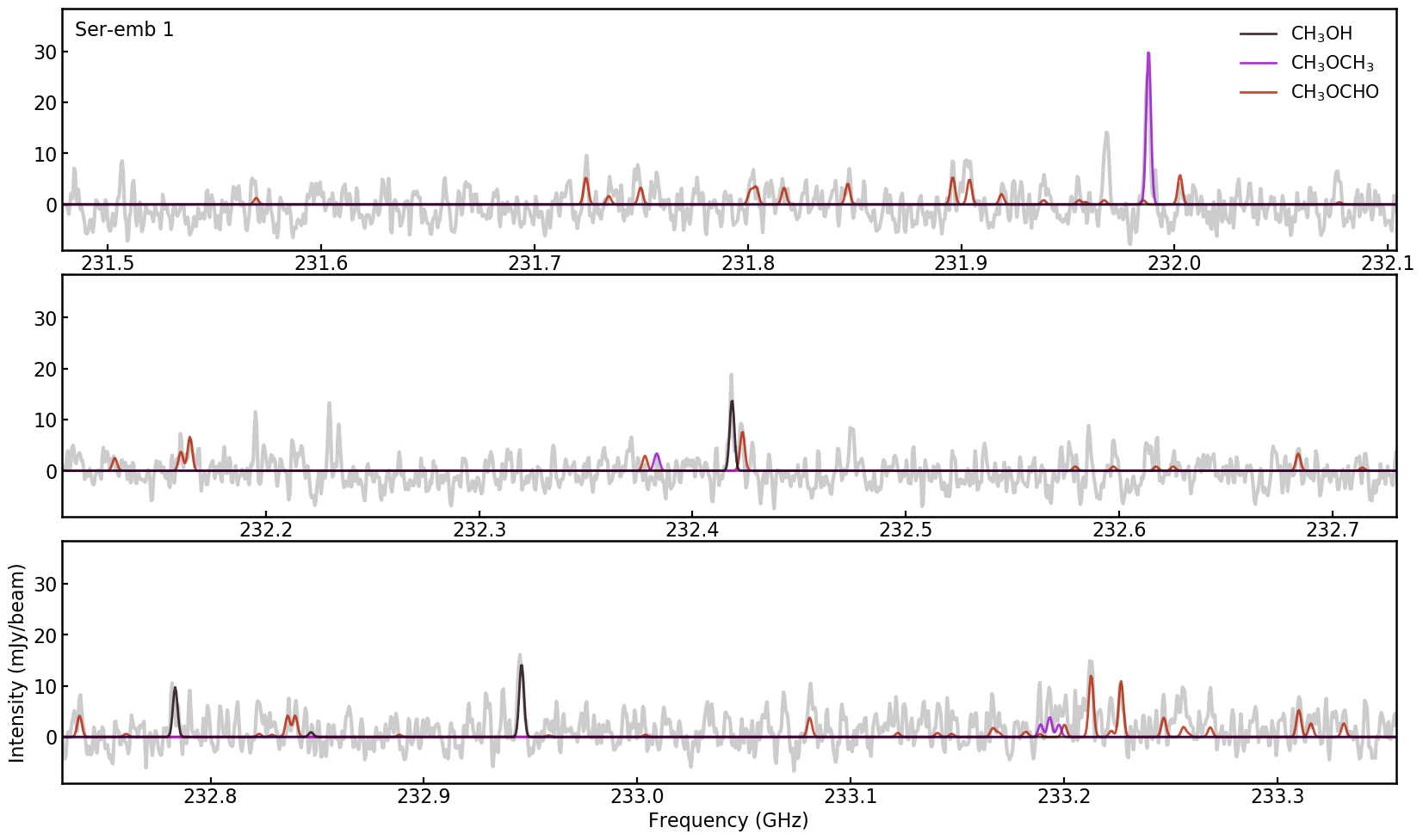
(a)

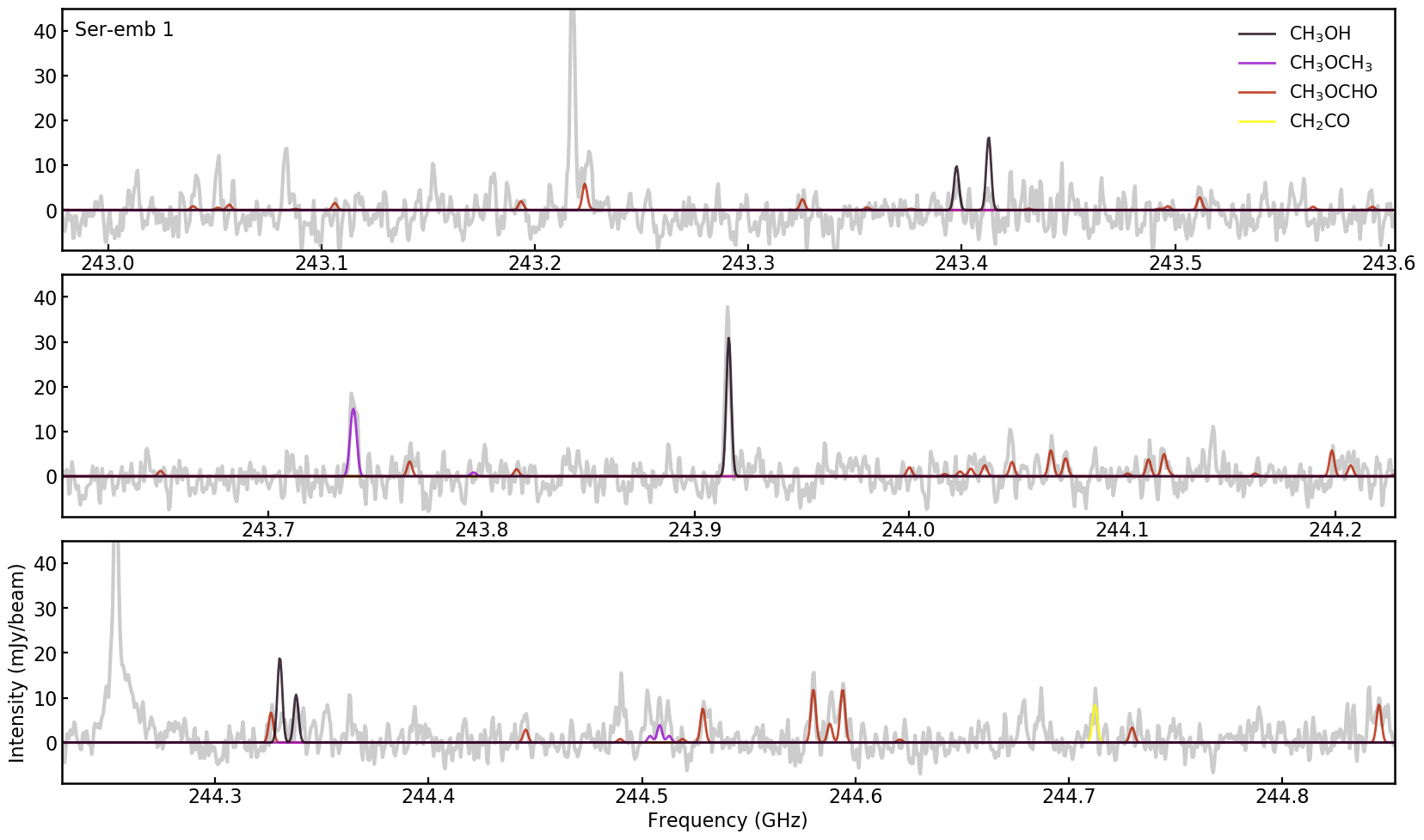
(b)

Figure 15: Full spectrum extracted from the continuum peak pixel in Ser-emb 1 (grey line), along with synthetic spectra of the detected COMs (colored lines). Spectra are calculated assuming the CH₃OH rotational temperature.

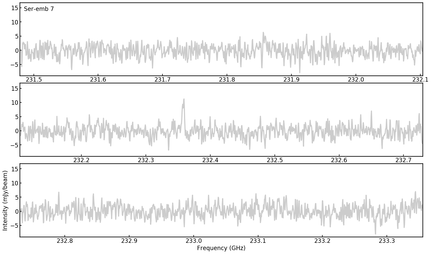
(a)

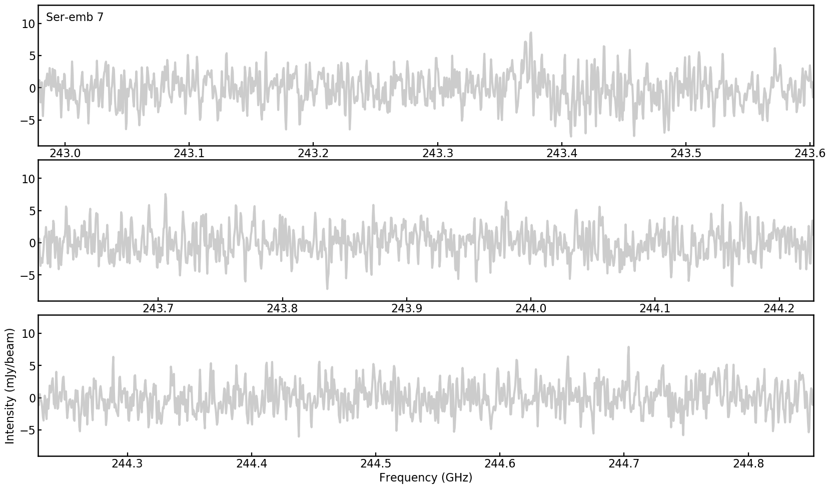
(b)

Figure 16: Full spectrum extracted from the continuum peak pixel in Ser-emb 7 (grey line).

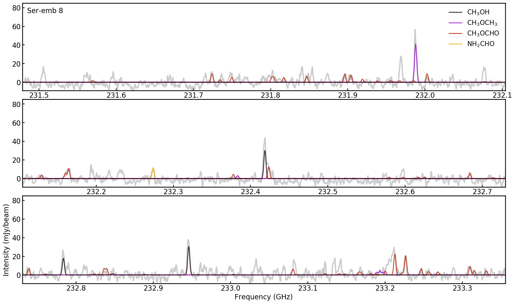
(a)

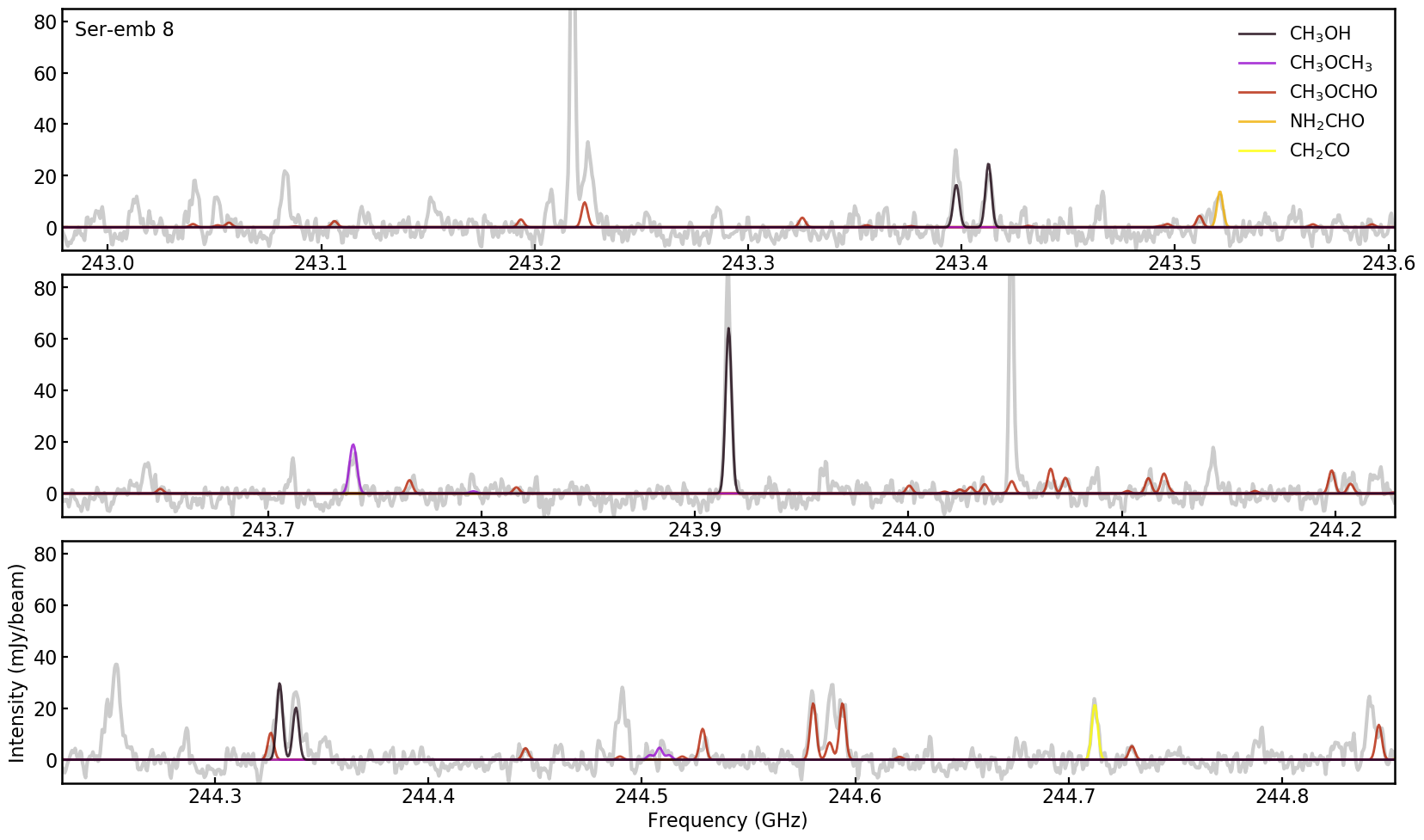
(b)

Figure 17: Full spectrum extracted from the continuum peak pixel in Ser-emb 8 (grey line), along with synthetic spectra of the detected COMs (colored lines). Spectra are calculated assuming the CH₃OH rotational temperature.

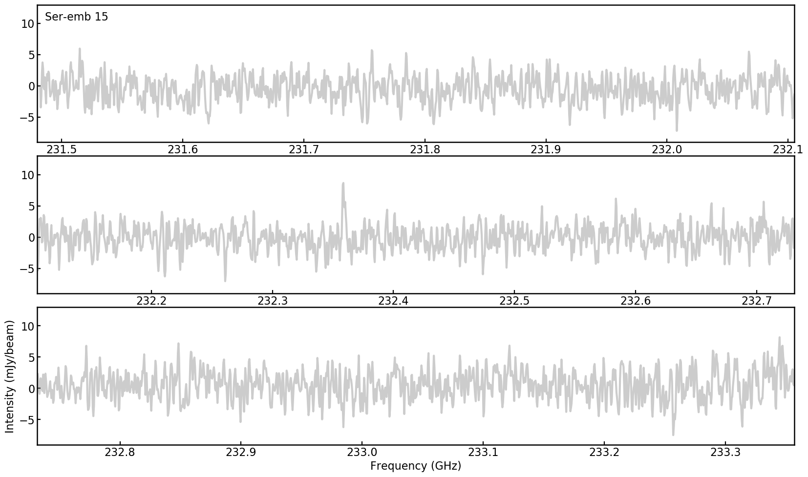
(a)

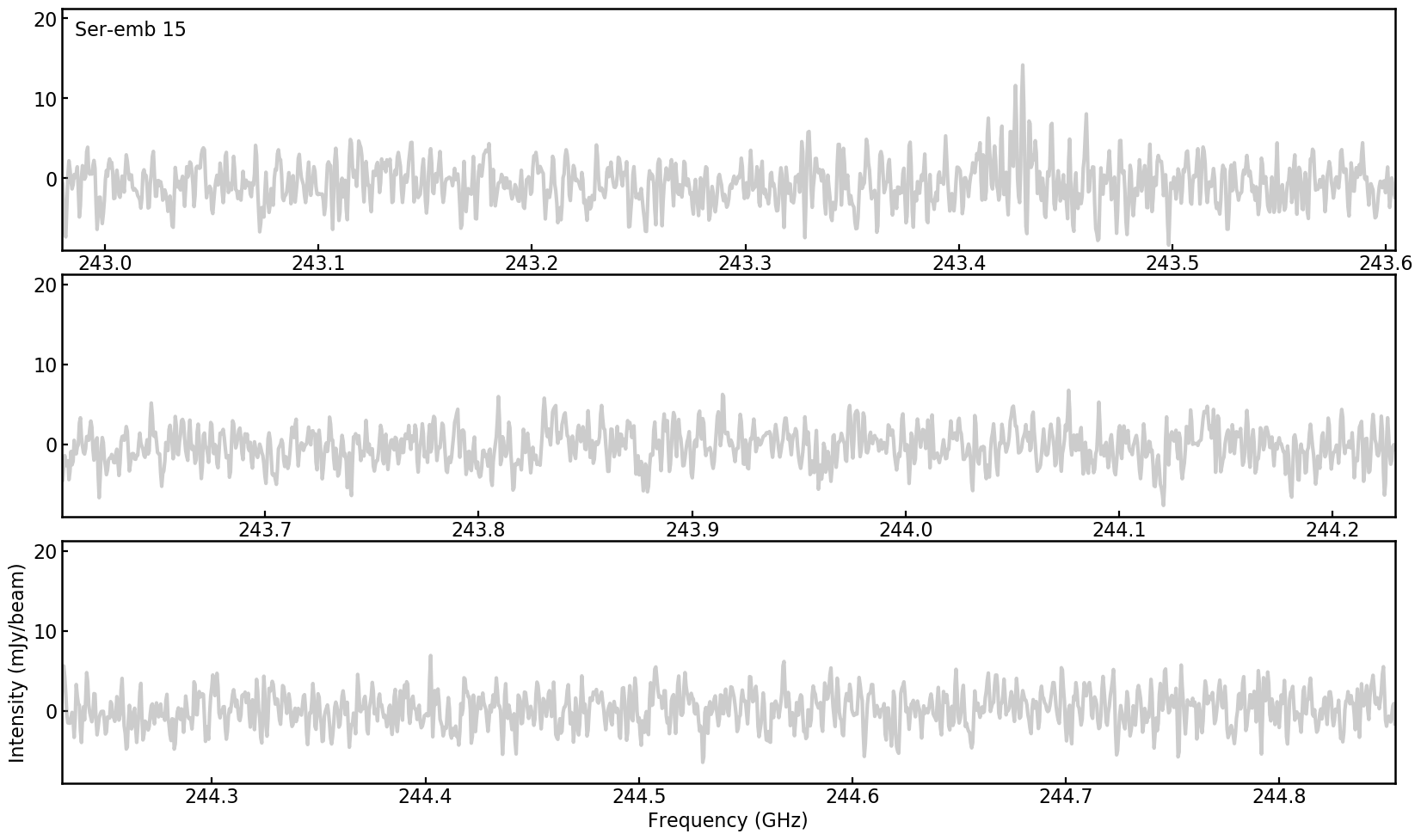
(b)

Figure 18: Full spectrum extracted from the continuum peak pixel in Ser-emb 15 (grey line).

References

- ALMA Partnership et al. (2015) ALMA Partnership, Brogan, C. L., Pérez, L. M., et al. 2015, Astrophys. J. Lett., 808, L3, doi: 10.1088/2041-8205/808/1/L3
- Altwegg et al. (2017) Altwegg, K., Balsiger, H., Berthelier, J. J., et al. 2017, Philosophical Transactions of the Royal Society of London Series A, 375, 20160253, doi: 10.1098/rsta.2016.0253
- Andre et al. (1993) Andre, P., Ward-Thompson, D., & Barsony, M. 1993, Astrophys. J., 406, 122, doi: 10.1086/172425
- Andrews et al. (2018) Andrews, S. M., Huang, J., Pérez, L. M., et al. 2018, Astrophys. J. Lett., 869, L41, doi: 10.3847/2041-8213/aaf741
- Astropy Collaboration et al. (2013) Astropy Collaboration, Robitaille, T. P., Tollerud, E. J., et al. 2013, Astron. Astrophys., 558, A33, doi: 10.1051/0004-6361/201322068
- Balucani et al. (2015) Balucani, N., Ceccarelli, C., & Taquet, V. 2015, Mon. Not. R. Astron. Soc., 449, L16, doi: 10.1093/mnrasl/slv009
- Beckwith & Sargent (1993) Beckwith, S. V. W., & Sargent, A. I. 1993, Astrophys. J., 402, 280, doi: 10.1086/172131
- Bergner et al. (2018) Bergner, J. B., Guzmán, V. G., Öberg, K. I., Loomis, R. A., & Pegues, J. 2018, Astrophys. J., 857, 69, doi: 10.3847/1538-4357/aab664
- Bergner et al. (2017) Bergner, J. B., Öberg, K. I., Garrod, R. T., & Graninger, D. M. 2017, Astrophys. J., 841, 120, doi: 10.3847/1538-4357/aa72f6
- Biver et al. (2014) Biver, N., Bockelée-Morvan, D., Debout, V., et al. 2014, Astron. Astrophys., 566, L5, doi: 10.1051/0004-6361/201423890
- Biver et al. (2015) Biver, N., Bockelée-Morvan, D., Moreno, R., et al. 2015, Science Advances, 1, 1500863, doi: 10.1126/sciadv.1500863
- Bockelée-Morvan et al. (2000) Bockelée-Morvan, D., Lis, D. C., Wink, J. E., et al. 2000, Astron. Astrophys., 353, 1101
- Bottinelli et al. (2007) Bottinelli, S., Ceccarelli, C., Williams, J. P., & Lefloch, B. 2007, Astron. Astrophys., 463, 601, doi: 10.1051/0004-6361:20065139
- Bottinelli et al. (2004) Bottinelli, S., Ceccarelli, C., Lefloch, B., et al. 2004, Astrophys. J., 615, 354, doi: 10.1086/423952
- Brown et al. (1990) Brown, R. D., Godfrey, P. D., McNaughton, D., Pierlot, A. P., & Taylor, W. H. 1990, Journal of Molecular Spectroscopy, 140, 340, doi: 10.1016/0022-2852(90)90146-H
- Cazaux et al. (2003) Cazaux, S., Tielens, A. G. G. M., Ceccarelli, C., et al. 2003, Astrophys. J. Lett., 593, L51, doi: 10.1086/378038
- Chandler & Richer (2000) Chandler, C. J., & Richer, J. S. 2000, Astrophys. J., 530, 851, doi: 10.1086/308401
- Choi et al. (2010) Choi, M., Tatematsu, K., & Kang, M. 2010, Astrophys. J. Lett., 723, L34, doi: 10.1088/2041-8205/723/1/L34
- Codella et al. (2014) Codella, C., Cabrit, S., Gueth, F., et al. 2014, Astron. Astrophys., 568, L5, doi: 10.1051/0004-6361/201424103
- Codella et al. (2016) Codella, C., Ceccarelli, C., Bianchi, E., et al. 2016, Mon. Not. R. Astron. Soc., 462, L75, doi: 10.1093/mnrasl/slw127
- Codella et al. (2017) Codella, C., Ceccarelli, C., Caselli, P., et al. 2017, Astron. Astrophys., 605, L3, doi: 10.1051/0004-6361/201731249
- Crovisier et al. (2004) Crovisier, J., Bockelée-Morvan, D., Colom, P., et al. 2004, Astron. Astrophys., 418, 1141, doi: 10.1051/0004-6361:20035688
- Di Francesco et al. (2001) Di Francesco, J., Myers, P. C., Wilner, D. J., Ohashi, N., & Mardones, D. 2001, Astrophys. J., 562, 770, doi: 10.1086/323854
- Dunham et al. (2014) Dunham, M. M., Stutz, A. M., Allen, L. E., et al. 2014, Protostars and Planets VI, 195, doi: 10.2458/azu_uapress_9780816531240-ch009
- Endres et al. (2009) Endres, C. P., Drouin, B. J., Pearson, J. C., et al. 2009, Astron. Astrophys., 504, 635, doi: 10.1051/0004-6361/200912409
- Enoch et al. (2009) Enoch, M. L., Evans, II, N. J., Sargent, A. I., & Glenn, J. 2009, Astrophys. J., 692, 973, doi: 10.1088/0004-637X/692/2/973
- Enoch et al. (2011) Enoch, M. L., Corder, S., Duchêne, G., et al. 2011, Astrophys. J., Suppl. Ser., 195, 21, doi: 10.1088/0067-0049/195/2/21
- Favre et al. (2014) Favre, C., Carvajal, M., Field, D., et al. 2014, Astrophys. J., Suppl. Ser., 215, 25, doi: 10.1088/0067-0049/215/2/25
- Favre et al. (2018) Favre, C., Fedele, D., Semenov, D., et al. 2018, Astrophys. J. Lett., 862, L2, doi: 10.3847/2041-8213/aad046
- Foreman-Mackey et al. (2013) Foreman-Mackey, D., Hogg, D. W., Lang, D., & Goodman, J. 2013, PASP, 125, 306, doi: 10.1086/670067
- Garrod & Herbst (2006) Garrod, R. T., & Herbst, E. 2006, Astron. Astrophys., 457, 927, doi: 10.1051/0004-6361:20065560
- Garrod et al. (2008) Garrod, R. T., Widicus Weaver, S. L., & Herbst, E. 2008, Astrophys. J., 682, 283, doi: 10.1086/588035
- Geppert et al. (2006) Geppert, W. D., Hamberg, M., Thomas, R. D., et al. 2006, Faraday Discussions, 133, 177, doi: 10.1039/B516010C
- Goldsmith & Langer (1999) Goldsmith, P. F., & Langer, W. D. 1999, Astrophys. J., 517, 209, doi: 10.1086/307195
- Groner et al. (1998) Groner, P., Albert, S., Herbst, E., & De Lucia, F. C. 1998, Astrophys. J., 500, 1059, doi: 10.1086/305757
- Guarnieri & Huckaufa (2003) Guarnieri, A., & Huckaufa, A. 2003, Zeitschrift Naturforschung Teil A, 58, 275, doi: 10.1515/zna-2003-5-603
- Harsono et al. (2018) Harsono, D., Bjerkeli, P., van der Wiel, M. H. D., et al. 2018, Nature Astronomy, 2, 646, doi: 10.1038/s41550-018-0497-x
- Harsono et al. (2014) Harsono, D., Jørgensen, J. K., van Dishoeck, E. F., et al. 2014, Astron. Astrophys., 562, A77, doi: 10.1051/0004-6361/201322646
- Herbst & van Dishoeck (2009) Herbst, E., & van Dishoeck, E. F. 2009, Annu. Rev. Astron. Astrophys., 47, 427, doi: 10.1146/annurev-astro-082708-101654
- Horn et al. (2004) Horn, A., Møllendal, H., Sekiguchi, O., et al. 2004, Astrophys. J., 611, 605, doi: 10.1086/422137
- Hunter (2007) Hunter, J. D. 2007, Computing in Science and Engineering, 9, 90, doi: 10.1109/MCSE.2007.55
- Ilyushin et al. (2009) Ilyushin, V., Kryvda, A., & Alekseev, E. 2009, Journal of Molecular Spectroscopy, 255, 32, doi: 10.1016/j.jms.2009.01.016
- Imai et al. (2016) Imai, M., Sakai, N., Oya, Y., et al. 2016, Astrophys. J. Lett., 830, L37, doi: 10.3847/2041-8205/830/2/L37
- Jacobsen et al. (2018) Jacobsen, S. K., Jørgensen, J. K., Di Francesco, J., et al. 2018, arXiv e-prints, arXiv:1809.00390
- Jones et al. (2001) Jones, E., Oliphant, T., Peterson, P., et al. 2001, SciPy: Open source scientific tools for Python. http://www.scipy.org/
- Jørgensen et al. (2005) Jørgensen, J. K., Bourke, T. L., Myers, P. C., et al. 2005, Astrophys. J., 632, 973, doi: 10.1086/433181
- Jørgensen et al. (2012) Jørgensen, J. K., Favre, C., Bisschop, S. E., et al. 2012, Astrophys. J. Lett., 757, L4, doi: 10.1088/2041-8205/757/1/L4
- Jørgensen et al. (2016) Jørgensen, J. K., van der Wiel, M. H. D., Coutens, A., et al. 2016, Astron. Astrophys., 595, A117, doi: 10.1051/0004-6361/201628648
- Jørgensen et al. (2018) Jørgensen, J. K., Müller, H. S. P., Calcutt, H., et al. 2018, Astron. Astrophys., 620, A170, doi: 10.1051/0004-6361/201731667
- Kristensen et al. (2012) Kristensen, L. E., van Dishoeck, E. F., Bergin, E. A., et al. 2012, Astron. Astrophys., 542, A8, doi: 10.1051/0004-6361/201118146
- Kryvda et al. (2009) Kryvda, A. V., Gerasimov, V. G., Dyubko, S. F., Alekseev, E. A., & Motiyenko, R. A. 2009, Journal of Molecular Spectroscopy, 254, 28, doi: 10.1016/j.jms.2008.12.001
- Lada (1987) Lada, C. J. 1987, in IAU Symposium, Vol. 115, Star Forming Regions, ed. M. Peimbert & J. Jugaku, 1–17
- Le Roy et al. (2015) Le Roy, L., Altwegg, K., Balsiger, H., et al. 2015, Astron. Astrophys., 583, A1, doi: 10.1051/0004-6361/201526450
- Lee et al. (2014) Lee, C.-F., Hirano, N., Zhang, Q., et al. 2014, Astrophys. J., 786, 114, doi: 10.1088/0004-637X/786/2/114
- Lefloch et al. (2018) Lefloch, B., Bachiller, R., Ceccarelli, C., et al. 2018, Mon. Not. R. Astron. Soc., 477, 4792, doi: 10.1093/mnras/sty937
- Loomis et al. (2018) Loomis, R. A., Cleeves, L. I., Öberg, K. I., et al. 2018, Astrophys. J., 859, 131, doi: 10.3847/1538-4357/aac169
- Maeda et al. (2008) Maeda, A., Lucia, F. C. D., & Herbst, E. 2008, Journal of Molecular Spectroscopy, 251, 293 , doi: https://doi.org/10.1016/j.jms.2008.03.014
- Marcelino et al. (2018) Marcelino, N., Gerin, M., Cernicharo, J., et al. 2018, Astron. Astrophys., 620, A80, doi: 10.1051/0004-6361/201731955
- Martin-Domenech et al. (2019) Martin-Domenech, R., Bergner, J. B., Oberg, K. I., & Jorgensen, J. K. 2019, arXiv e-prints, arXiv:1906.08848. https://arxiv.org/abs/1906.08848
- Maury et al. (2014) Maury, A. J., Belloche, A., André, P., et al. 2014, Astron. Astrophys., 563, L2, doi: 10.1051/0004-6361/201323033
- Müller et al. (2005) Müller, H. S. P., Schlöder, F., Stutzki, J., & Winnewisser, G. 2005, Journal of Molecular Structure, 742, 215, doi: 10.1016/j.molstruc.2005.01.027
- Müller et al. (2001) Müller, H. S. P., Thorwirth, S., Roth, D. A., & Winnewisser, G. 2001, Astron. Astrophys., 370, L49, doi: 10.1051/0004-6361:20010367
- Mumma & Charnley (2011) Mumma, M. J., & Charnley, S. B. 2011, Annu. Rev. Astron. Astrophys., 49, 471, doi: 10.1146/annurev-astro-081309-130811
- Öberg et al. (2009) Öberg, K. I., Garrod, R. T., van Dishoeck, E. F., & Linnartz, H. 2009, Astron. Astrophys., 504, 891, doi: 10.1051/0004-6361/200912559
- Öberg et al. (2015) Öberg, K. I., Guzmán, V. V., Furuya, K., et al. 2015, Nature, 520, 198, doi: 10.1038/nature14276
- Oesterling et al. (1999) Oesterling, L. C., Albert, S., De Lucia, F. C., Sastry, K. V. L. N., & Herbst, E. 1999, Astrophys. J., 521, 255, doi: 10.1086/307543
- Ortiz-León et al. (2018) Ortiz-León, G. N., Loinard, L., Dzib, S. A., et al. 2018, Astrophys. J. Lett., 869, L33, doi: 10.3847/2041-8213/aaf6ad
- Oya et al. (2016) Oya, Y., Sakai, N., López-Sepulcre, A., et al. 2016, Astrophys. J., 824, 88, doi: 10.3847/0004-637X/824/2/88
- Oya et al. (2017) Oya, Y., Sakai, N., Watanabe, Y., et al. 2017, Astrophys. J., 837, 174, doi: 10.3847/1538-4357/aa6300
- PICKETT et al. (1998) PICKETT, H., POYNTER, R., COHEN, E., et al. 1998, Journal of Quantitative Spectroscopy and Radiative Transfer, 60, 883 , doi: https://doi.org/10.1016/S0022-4073(98)00091-0
- Plummer et al. (1984) Plummer, G. M., Herbst, E., De Lucia, F., & Blake, G. A. 1984, Astrophys. J., Suppl. Ser., 55, 633, doi: 10.1086/190972
- Sakai et al. (2014) Sakai, N., Sakai, T., Hirota, T., et al. 2014, Nature, 507, 78, doi: 10.1038/nature13000
- Skouteris et al. (2019) Skouteris, D., Balucani, N., Ceccarelli, C., et al. 2019, Mon. Not. R. Astron. Soc., 482, 3567, doi: 10.1093/mnras/sty2903
- Skouteris et al. (2017) Skouteris, D., Vazart, F., Ceccarelli, C., et al. 2017, Mon. Not. R. Astron. Soc., 468, L1, doi: 10.1093/mnrasl/slx012
- Taquet et al. (2015) Taquet, V., López-Sepulcre, A., Ceccarelli, C., et al. 2015, Astrophys. J., 804, 81, doi: 10.1088/0004-637X/804/2/81
- van der Walt et al. (2011) van der Walt, S., Colbert, S. C., & Varoquaux, G. 2011, Computing in Science and Engineering, 13, 22, doi: 10.1109/MCSE.2011.37
- Walsh et al. (2016) Walsh, C., Loomis, R. A., Öberg, K. I., et al. 2016, Astrophys. J. Lett., 823, L10, doi: 10.3847/2041-8205/823/1/L10
- Winnewisser et al. (1985) Winnewisser, M., Winnewisser, B. P., & Winnewisser, G. 1985, in NATO Advanced Science Institutes (ASI) Series C, Vol. 157, NATO Advanced Science Institutes (ASI) Series C, ed. G. H. F. Diercksen, W. F. Huebner, & P. W. Langhoff, 375–402
- Xu et al. (2008) Xu, L.-H., Fisher, J., Lees, R. M., et al. 2008, Journal of Molecular Spectroscopy, 251, 305, doi: 10.1016/j.jms.2008.03.017
- Yen et al. (2015) Yen, H.-W., Takakuwa, S., Koch, P. M., et al. 2015, Astrophys. J., 812, 129, doi: 10.1088/0004-637X/812/2/129
- Zhang et al. (2018) Zhang, S., Zhu, Z., Huang, J., et al. 2018, Astrophys. J. Lett., 869, L47, doi: 10.3847/2041-8213/aaf744