Heavy metals in intermediate He-rich hot subdwarfs:
The chemical composition of HZ 44 and HD 127493

Abstract

Context. Hot subluminous stars can be spectroscopically classified as subdwarf B (sdB) and O (sdO) stars. While the latter are predominantly hydrogen deficient, the former are mostly helium deficient. The atmospheres of most sdOs are almost devoid of hydrogen, whereas a small group of hot subdwarf stars of mixed H/He composition exists, showing extreme metal abundance anomalies. Whether such intermediate helium-rich (iHe) subdwarf stars provide an evolutionary link between the dominant classes is an open question.

Aims. The presence of strong Ge, Sn, and Pb lines in the UV spectrum of HZ 44 suggests a strong enrichment of heavy elements in this iHe-sdO star and calls for a detailed quantitative spectral analysis focusing on trans-iron elements.

Methods. Non-LTE model atmospheres and synthetic spectra calculated with TLUSTY/SYNSPEC are combined with high-quality optical, UV and FUV spectra of HZ 44 and its hotter sibling HD 127493 to determine their atmospheric parameters and metal abundance patterns.

Results. By collecting atomic data from literature we succeeded to determine abundances of 29 metals in HZ 44, including the trans-iron elements Ga, Ge, As, Se, Zr, Sn, and Pb and provide upper limits for 10 other metals. This makes it the best described hot subdwarf in terms of chemical composition. For HD 127493 the abundance of 15 metals, including Ga, Ge, and Pb and upper limits for another 16 metals were derived. Heavy elements turn out to be overabundant by one to four orders of magnitude with respect to the Sun. Zr and Pb are among the most enriched elements.

Conclusions. The C, N, and O abundance for both stars can be explained by nucleosynthesis of hydrogen burning in the CNO cycle along with their helium enrichment. On the other hand, the heavy-element anomalies are unlikely to be caused by nucleosynthesis. Instead diffusion processes are evoked with radiative levitation overcoming gravitational settlement of the heavy elements.

1 Introduction

Hot subdwarf stars of spectral type O and B (sdO and sdB) represent late stages of the evolution of low-mass stars. They are characterized by high effective temperatures, ranging from $T_{\mathrm{eff}}=20\,000$ K to more than 45 000 K while their surface gravities are typically between $\log g=5.0$ and 6.5 (Heber, 2016). The vast majority of sdB stars are helium-deficient with helium abundances that can reach as low as $\log n(\mathrm{He})/n(\mathrm{H})=-4$ (Lisker et al., 2005). Most of these stars are evolving through the core helium-burning phase on the horizontal branch but their remaining hydrogen envelope is too thin to sustain hydrogen shell burning (Dorman et al., 1993). This is why they are said to populate the extreme part of the horizontal branch (EHB) in the Hertzsprung-Russell diagram. Since the mass of sdB stars is largely dominated by that of the He-burning core (the hydrogen envelope contributes less than 2%), the mass distribution of these stars is strongly peaked around the mass required for the He-flash ($\sim$0.47 $M_{\odot}$; Dorman et al. 1993; Han et al. 2002; Fontaine et al. 2012). Unlike normal horizontal branch objects, the sdB stars, due to their lack of H-shell burning, evolve directly to the white dwarf (WD) cooling sequence without an excursion to the asymptotic giant branch (AGB) (Dorman et al., 1993).
The formation and evolutionary history of the sdO stars is not understood very well. Because most sdO stars are hotter and somewhat more luminous than the sdB stars, they can not be associated to the EHB. Whether their evolution is linked to the EHB or not remains an open question. It has been suggested that the He-deficient sdO stars are the descendants of the sdB stars, because they share the peculiar chemical composition (Heber, 2016). However, the majority of sdO stars have atmospheres dominated by helium with hydrogen being a trace element only. The formation of these He-sdO stars is unlikely to be linked to the EHB and two rivaling scenarios have been invoked to explain the hydrogen deficiency, either via internal mixing (Lanz et al., 2004; Miller Bertolami et al., 2008) or via a merger of two helium white dwarfs (Zhang & Jeffery, 2012). A very small number of hot subluminous stars have atmospheres of mixed H/He composition. Because their metal content is very different from that of the extremely He-rich subdwarfs, Naslim et al. (2013) suggested to distinguish intermediate H/He composition subdwarfs (iHe-sds) with $n(\mathrm{He})/n(\mathrm{H})<4$ as a class separate from the extremely He-rich (eHe) hot subdwarfs. The SPY project has provided the largest homogeneous sample of hot subdwarfs from high resolution spectroscopy. By quantitative spectral analyses 85 H-rich hot subdwarf stars have been identified, as well as 23 eHe and 10 iHe hot subdwarfs (Lisker et al., 2005; Stroeer et al., 2007; Hirsch, 2009). The latter appear as a transition stage between the cooler H-rich sdB stars and the hotter eHe subdwarf stars (see Fig. 1). As to the carbon and nitrogen abundances a dichotomy exists, both for the eHe and the iHe sds. Stroeer et al. (2007) classified the line spectra of helium-rich hot subdwarfs in three classes: N-, C-, and C$\&$N-strong. Hirsch (2009) showed that, indeed, the N strong-lined stars are enriched in nitrogen with respect to the Sun, as are the C strong-lined enriched in carbon and the C&N strong-lined in both elements. This dichotomy is most obvious for the eHe hot subdwarf stars, the N-strong ones being mostly cooler than the C- or C$\&$N- strong ones. For the iHe hot subdwarfs such a separation is less pronounced (see Fig. 1).

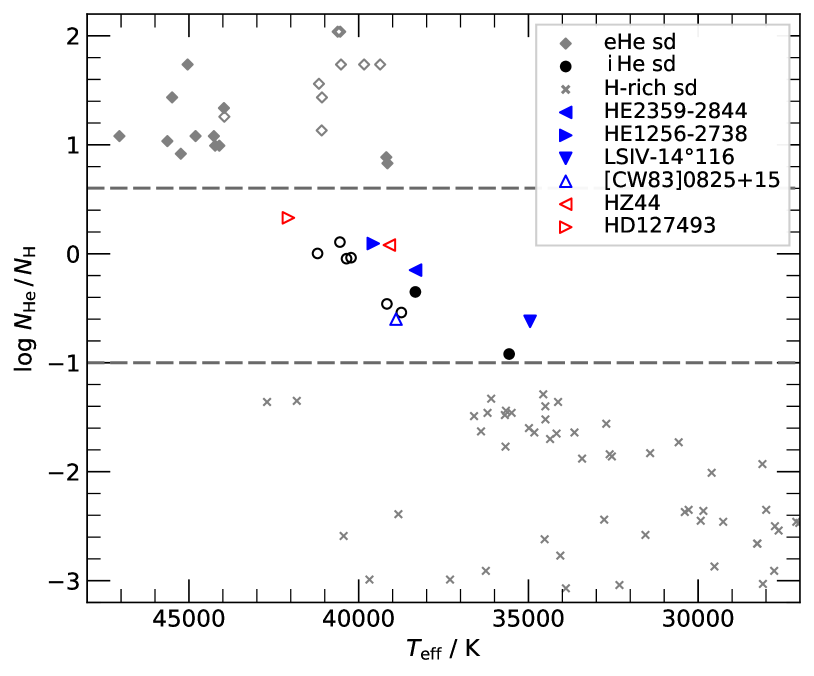
Figure 1: Distribution of helium abundance versus $T_{\mathrm{eff}}$ for the subdwarf population from the SPY sample (Lisker et al., 2005; Stroeer et al., 2007; Hirsch, 2009). The dashed lines mark the range of iHe subdwarfs. The two heavy-metal subdwarfs from SPY (Naslim et al., 2013) and the prototypical heavy-metal subdwarfs LS IV$-14^{\circ}116$ (Naslim et al., 2011) and [CW83] 0825$+$15 (Jeffery et al., 2017) are marked by blue triangles, HD 127493 and HZ 44 in red. Open symbols represent C-poor, N-rich stars, filled symbols C-rich stars.

Naslim et al. (2011) have discovered trans-iron elements, in particular zirconium and lead, to be strongly overabundant in the iHe-sdB LS IV$-14^{\circ}116$. Since then, three additional intermediate He-sdBs (indicated with blue triangles in Fig. 1), with effective temperature between 35 000 K and 40 000 K, have been found to be extremely enriched in heavy elements (Naslim et al., 2013; Jeffery et al., 2017). The origin of the extreme enrichment observed in iHe hot subdwarfs is not yet understood. Radiatively driven diffusion has been proposed, but is poorly constrained with only four stars ([CW83] 0825+15, LS IV$-14^{\circ}116$, and the SPY objects HE 2359–2844 and HE 1256–2738) studied so far. Therefore, we decided to extend the sample to higher temperatures by studying HZ 44 (39 000 K) and HD 127493 (42 000 K) for which excellent high-resolution spectroscopy is available both for the optical and the ultraviolet spectral range. This makes them excellent targets to perform a comprehensive quantitative abundance analysis and focus on trans-iron elements.
HZ 44 and HD 127493 were among the first sdOs to be identified in the 1950s. HZ 44 was discovered in the first survey for faint blue stars in the halo by Humason & Zwicky (1947). The first spectral analysis of the helium line spectrum of HZ 44 was published in the pioneering paper of Münch (1958). From a curve of growth analysis Peterson (1970) derived metal abundances for the first time, but we know of no contemporary study. HZ 44 is now a spectrophotometric standard star (Massey et al., 1988; Oke, 1990; Landolt & Uomoto, 2007a), used for the calibration of the HST (Bohlin et al., 1990; Bohlin, 1996; Bohlin et al., 2001), as well as that of Gaia (Marinoni et al., 2016), and therefore has frequently been observed. High resolution spectra are available from the far-UV to the red in the FUSE, IUE, and HIRES@Keck data archives.
HD 127493 has been used as secondary spectrophotometric standard star (Spencer Jones, 1985; Kilkenny et al., 1998; Bessell, 1999). Therefore, very accurate photometry is available but spectroscopic observations are not as extensive as for HZ 44. Starting with the curve of growth analyses of Peterson (1970) and Tomley (1970) abundances of C, N, O, Ne, Mg, and Si were derived. The first NLTE model atmospheres were calculated by Kudritzki (1976), who revised the atmospheric parameters. Abundances of carbon (Gruschinske et al., 1980) and C, N, O and Si (Simon et al., 1980) were derived from equivalent widths of ultraviolet lines. A NLTE analyis of optical spectra allowed Bauer & Husfeld (1995) to determine the abundances of C, N, O, Ne, Mg, Al, and Si. The most recent NLTE analysis by Hirsch (2009) revised the atmospheric parameters and determined C and N abundances from optical spectra. For completeness we give a comparison of our results with those of previous analyses in the Appendix. Hence, our knowledge of the chemical composition of both stars is rather limited.
The paper is organized as follows. In Sect. 2 we provide a description of the available spectra followed by a presentation of the atmospheric parameters that we derived for our stars in Sect. 3. The spectroscopic masses obtained from the spectral energy distributions and the Gaia parallaxes are presented in Sect. 4. The atomic data used for our abundance analysis are discussed in Sect. 5. In Sect. 6 we provide details on the abundance analysis of all considered metallic elements. The abundance patterns for HZ 44 and HD 127493 are discussed in Sect. 7 and we conclude in Sect. 8.

2 Spectroscopic observations

Table 1: Spectra used for the analysis.

Star	Instrument	Range (Å)	R	S/N
HD 127493	IUE SWP	1150 $-$ 1970	10 000	114
	GHRS	1225 $-$ 1745	0.07 Å	140
	IUE LWR	1850 $-$ 3273	10 000	114
	FEROS	3700 $-$ 9200	48 000	$180$
HZ 44	FUSE	1905 $-$ 1188	19 000	130
	IUE SWP	1150 $-$ 1970	10 000	110
	HIRES	3022 $-$ 7580	36 000	$142$
	ISIS	3700 $-$ 5260	1.5 Å	$170$

For both stars excellent archival data are available in both the optical and UV ranges. An overview of the spectra we collected and used is given in Table $a$, with additional details on the individual observations listed in Table 7.
We used optical FEROS spectra to determine the atmospheric parameters of HD 127493 and measure photospheric metal abundances. FEROS is an echelle spectrograph mounted on the MPG/ESO-2.20m telescope operated by the European Southern Observatory (ESO) in La Silla. It features a high resolving power of $\mathrm{R}\approx 48000$ (Kaufer et al., 1999) and its usable spectral range, from $\sim$3700 Å to $\sim$9200 Å, includes all the Balmer lines as well as many He i, He ii, and metal lines. The three available spectra of HD 127493 were co-added to achieve a high signal-to-noise ratio (S/N) of $\gtrsim$ 100 in the 4000 – 6000 Å range. Nevertheless, the S/N decreases drastically toward both ends of the spectral range and especially below 3800 Å.
Both stars have been observed with the International Ultraviolet Explorer (IUE) satellite with the short-wavelength prime (SWP) camera. We retrieved three archival INES spectra for HD 127493 and two for HZ 44. For each star we co-added the individual spectra to increase the S/N. They continuously cover the 1150 – 1980 Å range with a resolution of $\mathrm{R}\approx 10000$. Additional IUE spectra taken with the LWR camera (covering the 1850 – 3350 Å range) are also available for both stars. However these spectra have a lower quality and the S/N drops sharply at both ends of the spectra. Fewer lines are observed in this wavelength range but the IUE LWR spectrum of HD 127493 has nevertheless been useful for the abundance analysis.
HD 127493 has also been observed with the Goddard High-Resolution Spectrograph (GHRS) mounted on the Hubble Space Telescope (HST). These spectra are publicly available in the MAST archive and cover the 1225 – 1745 Å range with a resolution of $\Delta\lambda\approx 0.07$ Å. The final spectrum is a combination of ten observations spanning 35 Å each and lacks coverage in the following regions: 1450.5 – 1532.5 Å, 1567.7 – 1623.2 Å, and 1658.1 – 1713.0 Å. Since the wavelength calibration was not perfect, we cross-correlated the individual spectra to match the synthetic spectrum of HD 127493. In addition, they were shifted to match the flux level of the IUE spectra.
HZ 44 has been observed with the Far Ultraviolet Spectroscopic Explorer (FUSE) satellite over the spectral range between 905 Å and 1188 Å. We retrieved three calibrated observations from MAST, two taken through the LWRS ($30"\times 30"$) aperture, and one through the MDRS ($4"\times 20"$) aperture. We co-added all spectra from the eight segments in each observation. After inspection it turned out that the MDRS spectrum had a better quality and a better wavelength calibration, so we use this spectrum for our analysis.

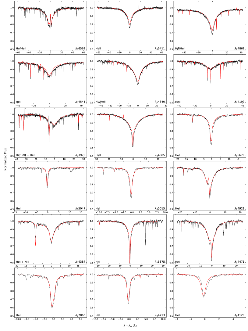
Figure 2: Best fit (red) to the Balmer and helium lines selected in the normalized FEROS spectrum of HD 127493 (black).

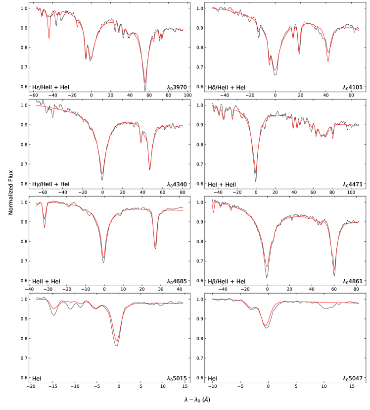
Figure 3: Best fit (red) to the Balmer and helium lines selected in the flux-calibrated ISIS spectrum of HZ 44 (black).

To determine the atmospheric parameters of HZ 44 we used a low resolution (1.5 Å), high S/N spectrum taken with the Intermediate dispersion Spectrograph and Imaging System (ISIS) mounted at the Cassegrain focus of the 4.2m William Herschel Telescope on La Palma. The spectrum covers the 3700$-$5260 Å range, thus including the Balmer lines, except H_α, as well as He i and ii lines.
The spectra of HZ 44 taken with the HIRES echelle spectrograph mounted on the Keck I telescope on Mauna Kea were most valuable for our abundance analysis. A total of 68 extracted HIRES spectra of HZ 44 from several programs covering various wavelength ranges are available in the Keck Observatory Archive (KOA). We co-added the spectra of four high S/N HIRES observations to produce the spectrum used for our abundance analysis. To access the ranges between 3022 Å and 3128 Å and above 5990 Å we considered two additional HIRES spectra that were used specifically for these regions. Additional spectra were also retrieved from the archive and used to measure radial velocities. Unfortunately, the normalization of HIRES spectra is difficult since the spectral orders are narrower than many broad Balmer or helium lines. This is not a problem for sharp metal lines, but renders the spectra next to useless for the determination of atmospheric parameters of HZ 44.

3 Atmospheric parameters and radial velocities

In order to analyze the spectra of our stars we computed non-LTE model atmospheres using the TLUSTY and SYNSPEC codes developed by Hubeny (1988) and Lanz & Hubeny (2003). A detailed description of TLUSTY/SYNSPEC has recently been published in Hubeny & Lanz (2017a, b, c).
We derived atmospheric parameters for both stars using optical spectra (besides HIRES) and a newly constructed model atmosphere grid that includes effective temperatures from $T_{\mathrm{eff}}=35\,000$ K to 48 000 K in steps of 1000 K and surface gravities from $\log g=$ 4.7 to 6.0 in steps of 0.1. For each of these combinations, models with helium abundances from $\log n_{\mathrm{He}}/n_{\mathrm{H}}=-1.0$ to $+2.1$ in steps of 0.1 were computed. All models in the grid include carbon, nitrogen, and silicon in non-LTE using the abundances determined by our previous analysis of HD 127493 (Dorsch et al., 2018) which significantly improves the atmospheric structure compared to models that only include hydrogen and helium (e. g. Schindewolf et al., 2018). These values of C, N, and Si are also appropriate for HZ 44 as shown in the abundance analysis presented in Sect. 6. The selection of all lines we used, as well as the global best-fit model for HD 127493 is shown in Fig. 2. Our final best fit of the ISIS spectrum of HZ 44 is shown in Fig. 3. The resulting parameters derived from the simultaneous fit of all selected H and He i-ii lines for both stars are reported in Table 2. The atmospheric parameters for HD 127493 derived by Hirsch (2009) are also listed. They were obtained with the same FEROS spectrum but different model atmospheres and are fully consistent with our results. As shown in Fig. 1 the atmospheric parameters of both stars fit very well the trend of helium abundance to increase with increasing effective temperatures. We found no indication of rotation or microturbulence in either star; some optical metal lines are in fact sharper in the observations than in the models.

Table 2: Parameters derived from optical spectroscopy.

Name	$T_{\text{eff}}$	$\log{g}$	$\log{n_{\mathrm{He}}/n_{\mathrm{H}}}$	v${}_{\rm rot}\sin{i}$	Spectrum	Ref
	[K]	[cgs]		[km s-1]
HZ 44	$39100\pm 600$	$5.64\pm 0.10$	$0.08\pm 0.05$	$<5$	ISIS	1
HD 127493	$42070\pm 180$	$5.61\pm 0.04$	$0.33\pm 0.06$	$<10$	FEROS	1
	$42480\pm 250$	$5.60\pm 0.05$	$0.60\pm 0.30$	$<10$	FEROS	2

Radial velocities of HZ 44 in 27 HIRES spectra taken between 1995 and 2016 were measured by Schork (2018) and are listed in Table 8. From these values an average radial velocity of $v_{\mathrm{rad}}=-12.7\pm 0.4$ km s^-1 was derived. The measurements show that the radial velocity of HZ 44 does not vary on a scale of a few km s^-1. Within the radial velocity uncertainties, neither a short- nor a long-period companion is detected. Our radial velocity measurement for HD 127493 is consistent with the value derived by Hirsch (2009) using the same FEROS spectrum ($-17\pm 3$ km s^-1).

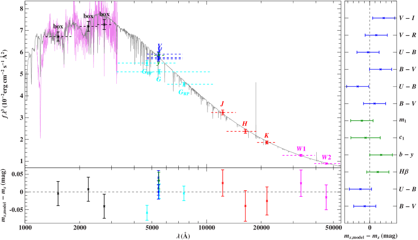
Figure 4: Comparison of synthetic spectra with photometric data for HZ 44 (top) and HD 127493 (bottom). The three black data points labeled “box” are binned fluxes from a low-dispersion IUE spectrum. Filter-averaged fluxes are shown as colored data points that were converted from observed magnitudes (the dashed horizontal lines indicate the respective filter widths), while the gray solid line represents a synthetic spectrum using the atmospheric parameters given in Table 2. The residual panels at the bottom and right hand side show the differences between synthetic and observed magnitudes/colors. The following color codes are used to identify the photometric systems: Johnson-Cousins (blue), Strömgren (green), Gaia (cyan), UKIDSS (rose), 2MASS (red), WISE (magenta).

4 Stellar masses, radii, and luminosities

With the release of Gaia DR2, high accuracy parallax ($\varpi$) and therefore distance measurements have become available for a large sample of hot subdwarfs. This allows us to derive more precise spectroscopic masses for these stars. We collected photometric measurements from several surveys and converted them into fluxes (see Tables 9 and 10). In addition, we use low-resolution, large-aperture IUE spectra that were averaged in three regions (1300–1800 Å, 2000–2500 Å, 2500–3000 Å) as “box filters” to cover the UV range. Our photometric fitting procedure is described in detail in Heber et al. (2018). The $\chi^{2}$ fitting procedure scales our final synthetic spectra to match the photometric data and has the solid angle $\theta=2R/D$ and the color excess $E_{B-V}$ as free parameters. Reddening is modeled with $R_{V}=3.1$ as the extinction parameter (a standard value for the diffuse ISM) and the corresponding mean extinction law from Fitzpatrick (1999). The resulting solid angle can be combined with the Gaia parallax distance to obtain the stellar radius, from which the stellar mass can be computed using the surface gravity derived from spectroscopy. The SED-fits are shown in Fig. 4 and the derived parameters in Table 3. Considering the non-detection of radial velocity variations and the evident lack of an IR excess, we can state that there is no indication of binarity in HZ 44. The SED of HD 127493 also shows no IR excess that would hint at a companion. The masses determined from the SED-fits are consistent with the canonical subdwarf mass, 0.47 $M_{\odot}$ (Fontaine et al., 2012, and references therein).

Table 3: Parallax and parameters derived from the SED fitting.

Results	HZ 44	HD 127493
$\varpi$ (mas)	$2.48\pm 0.08$	$5.82\pm 0.09$
$d$ (pc)	$403\pm 13$	$172\pm 3$
$\theta\,(10^{-11}\,\mathrm{rad})$	$2.134\pm 0.011$	$4.53\pm 0.03$
$E_{B-V}$	$0.010\pm 0.004$	$0.052\pm 0.004$
$R/R_{\odot}$	$0.191\pm 0.007$	$0.172\pm 0.003$
$M/M_{\odot}$	$0.59\pm 0.14$	$0.43\pm 0.05$
$L/L_{\odot}$	$77\pm 4$	$84\pm 2$

5 Atomic data

Table 4: Data for elements not included in the Kurucz line-list (gfall08oct17.dat).

Ion	$N_{\mathrm{UV}}$	$N_{\mathrm{VIS}}$	Reference
Ga iii	3	2	15, 2(28)
Ga iv	69	$-$	3
Ga v	37	$-$	3
Ge iii	1	$-$	1(25,18)
Ge iv	7	6	23, 2(28)
Ge v	24	$-$	3
As iii	$-$	$-$	1(26,19,17)
As iv	$-$	6	2(27), 1(25)
As v	2	$-$	1(19)
Se iv∗	3	$-$	1(22)
Se v∗	4	$-$	3
Kr iv∗	42	6	3
Kr v∗	$-$	$-$	3
Sr iv∗	109	1	3

Ion	$N_{\mathrm{UV}}$	$N_{\mathrm{VIS}}$	Reference
Sr v∗	23	$-$	3
Y iii∗	1	2	10, 16
Zr iv	11	8	3
Zr v	$-$	$-$	3
Mo iv∗	92	$-$	29,3
Mo v∗	69	$-$	3
Mo vi∗	5	$-$	3
In iii∗	5	$-$	4
Sn iii	$-$	$-$	13
Sn iv	7	$-$	4, 12
Sb iii∗	$-$	$-$	1(17)
Sb iv∗	1	$-$	1(20)
Sb v∗	2	$-$	4
Te iii∗	$-$	$-$	14

Ion	$N_{\mathrm{UV}}$	$N_{\mathrm{VIS}}$	Reference
Te v∗	1	$-$	1(30)
Te vi∗	2	$-$	3
Xe iv∗	5	$-$	3
Xe v∗	4	$-$	3
Ba v∗	2	$-$	3
Tl iii∗	$-$	$-$	5
Pb iii	2	$-$	7, 1(24)
Pb iv	17	9	11, 5, 8, 1(24)
Pb v	36	$-$	9
Bi iii∗	$-$	$-$	1(23)
Bi iv∗	$-$	$-$	1(21)
Bi v∗	1	$-$	5
Th iv∗	2	$-$	6

While atomic data and line lists for elements lighter than the iron-group are readily accessible via, for example, the Kurucz compilations and the NIST database, data for trans-iron elements are much more scarce. Since these elements are of special interest for the analysis of our two stars we invested particular effort into searching the literature and collecting data (energy levels, line positions, and oscillator strengths) for many trans-iron elements. We list in Table 4 the ions that we took into consideration as well as the references for their atomic data. We also include in this table, for each ion, the number of lines visible (with a predicted equivalent width greater than 5 mÅ) in the final model spectrum of HZ 44. The basis of our line list is the most recent line list published by Kurucz (2018) and available online. The list was further extended with data listed in ALL, the Atomic Line List (v2.05b21). In the context of their ongoing “Stellar Laboratories” series, Rauch et al. (2015) have published a large collection of atomic data for elements with $\mathrm{Z}\geq 30$ on the TOSSwebsite. While this collection was made for the analysis of hot white dwarfs with $T_{\mathrm{eff}}>60\,000$ K, it also includes atomic data for ions of stages iv-v that are observed in the sdOs discussed here. Thus, additional lines were added from TOSS and other theoretical works listed in Table 4. Finally the list was merged with the collection of lines from low-lying energy levels by Morton (2000) but preferring more recent data if available. Hyper-fine structure and isotopic line splitting are not considered because of the lack of atomic data. For subordinate lines the effect is expected to be small, but may be significant for resonance lines (e. g. Mashonkina et al., 2003) such as the Pb iv 1313 Å. Fortunately, for the latter resonance line atomic data are available for several isotopes and we included them in the line formation calculations (see O’Toole & Heber, 2006).

6 Metal abundance analysis

Table 5: Model atoms used for the final model of HZ 44 with their number of explicit levels (L) and superlevels (SL).

Ion	L	SL
H i	17	$-$
He i	24	$-$
He ii	20	$-$
C ii	34	15
C iii	34	12
C iv	35	12
N ii	32	10
N iii	40	19
N iv	34	14
N v	21	14
O ii	36	12
O iii	28	13
O iv	31	18
O v	34	16
O vi	15	15
Ne ii	23	19
Ne iii	22	12
Ne iv	10	12
Mg ii	21	14
Mg iii	37	13
Mg iv	29	15
Mg v	18	12
Al ii	20	19
Al iii	19	14

Ion	L	SL
Si ii	36	14
Si iii	31	15
Si iv	19	14
P iv	14	$-$
P v	13	14
S ii	23	10
S iii	29	12
S iv	33	15
S v	20	15
S vi	13	13
Ar ii	42	12
Ar iii	27	17
Ar iv	39	$-$
Ar v	25	$-$
Ca ii	32	$-$
Ca iii	15	14
Ca iv	17	14
Fe iii	$-$	50
Fe iv	$-$	43
Fe v	$-$	42
Ni iii	$-$	36
Ni iv	$-$	38
Ni v	$-$	48
Total	1062	506

Model atmospheres were calculated for each star using their atmospheric parameters as listed in Table 2. All ions for which model atoms are available are included in non-LTE (see Table 5), while the remaining elements are treated with the LTE approximation. The next higher ionization stage of each metal listed in Table 5 is considered as a one-level ion. More information on the model atoms we use can be found on the TLUSTY web site and in Lanz & Hubeny (2003, 2007). The Mg iii-v and Ar iv-v model atoms are described in Latour et al. (2013). The Ca iii-iv model atoms were constructed in a similar manner (P. Chayer, priv. comm.) while the Ca ii model atom is described in Allende Prieto et al. (2003). To compute the partition functions of heavy elements (Z$>$30) in ionization stages iv–vi we added atomic data from NIST to SYNSPEC, as in Chayer et al. (2006). As a starting point, abundances in the TLUSTY model were set to values estimated by eye for each element. Based on this preliminary model, a series of synthetic spectra with a range of abundances for each element were created with SYNSPEC. The abundance of the elements were determined one-by-one using the downhill-simplex fitting program SPAS developed by Hirsch (2009). This method works well for isolated lines but is not reliable for heavily blended lines, in particular in the UV region. The abundance for these elements was estimated by manually comparing models with the observation. Even with this method, the placement of the continuum (especially in the FUSE range) remains an important source of uncertainty. As noted by Pereira et al. (2006), the true continuum in the FUSE spectral region may be well above the highest observed fluxes. This complicates the continuum placement since some opacity (photospheric and interstellar) is still missing in our final synthetic spectra. Thus for some elements we could only derive upper limits. This includes elements having low abundances but also elements that show lines in the FUSE range only, where the aforementioned problems are most severe. For some elements in HD 127493 no abundances, or upper limits, could be derived (Cl, K, As, Se, Sb, Xe, Bi). This is due to insufficient spectral coverage: the elements in question have their strongest spectral lines in ranges where no data are available for that star (FUSE, UVA).
A summary of the photospheric abundances derived for HZ 44 and HD 127493 are presented at the end of this section in Fig. 12 and in Table 11. In addition, we include in Sect. A.3 a comparison between the final synthetic spectrum and the observed spectrum in all wavelength ranges for both stars. We note that for some elements, namely Ne, Ar, Cl, Sn, Tl, Pb, and Th, the uncertainty on their solar photospheric abundance (Asplund et al., 2009) contributes significantly to the total uncertainty when computing the ratio with solar abundances. The uncertainty stated on upper limits and by-eye abundances is defined as follows: at the upper bound the lines are judged to be clearly too strong, while they can not be distinguished from noise at the lower bound.
In the following subsections, we present in detail the result of our abundance analysis for each element. Light elements (C, N, O) are discussed in Sect. 6.1, intermediate elements (F, Ne, Na, Mg, Al, Si, P, S, Cl, Ar, K, Ca, Ti) in Sect. 6.2, iron-group elements treated in non-LTE (Fe, Ni) in Sect. 6.3, iron-group elements treated in LTE (V, Cr, Mn, Co, Cu, Zn) in Sect. 6.4, detected trans-iron elements (Ga, Ge, As, Se, Zr, Sn, Pb) in Sect. 6.5, and trans-iron elements with upper limits (Kr, Sr, Y, Mo, Sb, Te, Xe, Th) in Sect. 6.6. Finally, Sect. 6.7 addresses the elements for which we could not even assess an upper limit due to the weakness of their predicted lines (Sc, In, Ba, Tl, Bi). We then discuss the chemical portrait obtained for both stars in Sect. 6.8. In the rest of the paper we give our abundances as $\log n_{\mathrm{X}}/n_{\mathrm{H}}$ and use the shorter notation $\log\mathrm{X/H}$. Here, $n_{X}$ is the dimensionless number fraction. To put the abundances in perspective, we additionally state the corresponding number fraction relative to solar values $n_{\mathrm{X}}/n_{\mathrm{X},\odot}$.

6.1 Light metals (C, N, O)

The carbon abundance in HZ 44 was measured using nine optical C iii lines. The abundance derived this way, $\log\mathrm{C/H}=-4.31\pm 0.13$ ($8.6\times 10^{-2}$ times solar), is consistent with the strong C iii and C iv lines observed in the UV region. Carbon lines are weaker in the optical spectrum of HD 127493. We use the resonance doublet C iv $\lambda\lambda$ 1548, 1551 Å and the C iii sextuplet lines at 1175 Å to derive an abundance of $\log\mathrm{C/H}=-4.30\pm 0.08$ ($3.9\times 10^{-2}$ times solar).
The nitrogen abundances measured in HZ 44 from different ionization stages/lines in the optical region are not very consistent. Most N iii lines are well reproduced; some are too strong (e. g. N iii $\lambda\lambda$ 4378.99, 4379.20 Å) while few are too weak (e. g. N iii 4003.58 Å). We identified only one strong N iv line in the optical spectrum of HZ 44 (N iv 4057.76 Å) which fits the final model well. We measure an abundance of $\log\mathrm{N/H}=-2.39\pm 0.21$ ($29$ times solar) for HZ 44. However, many strong N ii lines are too broad and shallow in the model, even assuming a rotation velocity and microturbulence of 0 km s^-1 and were therefore excluded from the fit (e. g. N ii $\lambda\lambda\,$3995.00, 4041.31, 4236.91 Å). This may be related to numerical issues due to low population numbers. In HD 127493 the issues with some optical N ii lines are even more pronounced; they appear in emission in the model and were excluded from the fit. In addition to optical N iii-iv lines we used UV lines to constrain the abundance, including the N v $\lambda\lambda\,1238.8,1242.8$ Å resonance lines, the strong N iv 1718 Å line, and several N iii lines. All ionization stages give a consistent abundance of $\log\mathrm{N/H}=-2.09\pm 0.17$ (26 times solar).
The abundance of oxygen in HZ 44 was measured using optical O ii and O iii lines. Although these lines are weak compared to lines from other elements, they could be used to find an abundance of $\log\mathrm{O/H}=-3.77\pm 0.13$ ($12\times 10^{-2}$ times solar). The strongest observed O lines in the UV region (O iii 1150.884 Å in FUSE and O iv 1343.51 Å in the IUE/SWP spectrum) support this value. O iv $\lambda\lambda$ 1338.62, 1343.51 Å are observed in the GHRS spectrum of HD 127493 but blended with Ni lines. Since no optical lines were detected in that star we only set an upper limit of $\log\mathrm{O/H}\leq-4.3$ ($2\times 10^{-2}$ times solar) and note that the actual abundance is likely not significantly lower.

6.2 Intermediate metals (F to Ti)

For HZ 44, all elements from fluorine to titanium were analyzed. Due to the lack of UVA and FUSE spectra, P, Cl, Ar, K, and Ti could not be studied in HD 127493.
No fluorine lines are observed in HZ 44 which allows us to provide an upper limit of $\log\mathrm{F/H}\leq-5.0\pm 0.4$ ($130$ times solar) based on F ii $\lambda\lambda$ 3503.11, 3505.63, 3847.09, 3849.99, and 3851.67 Å. None of these F ii lines are strong enough in HD 127493 set a meaningful limit on the abundance.
The neon abundance measurement for HZ 44 is based on several strong Ne ii lines, which are weaker in HD 127493 due to its higher temperature. Most of them lie between 3300 Å and 3800 Å though some strong Ne ii lines exist at longer wavelengths. Fitting all accessible Ne lines results in $\log\mathrm{Ne/H}=-3.23\pm 0.11$ ($3.3$ times solar) for HZ 44 and $\log\mathrm{Ne/H}=-2.38\pm 0.18$ ($3.1$ times solar) for HD 127493. The weaker Ne iii lines are reasonably well reproduced with the abundance stated above.
Sodium lines are weak, but clearly visible in HZ 44, most notably Na ii $\lambda\lambda$ 3285.61, 3533.06, 3631.27, 4392.81 Å. We find $\log\mathrm{Na/H}=-4.43\pm 0.06$ (10 times solar) for HZ 44. Na ii $\lambda\lambda$ 4392.81, 4405.12 Å allow an upper limit of $\log\mathrm{Na/H}\leq-3.4\pm 0.3$ (48 times solar) to be set for HD 127493.
The strongest observed magnesium lines are by far the Mg ii triplet at 4481 Å. All other optical lines are too weak to be observed in either star. We derive $\log\mathrm{Mg/H}=-3.8\pm 0.2$ (1.9 times solar) for HZ 44 and $\log\mathrm{Mg/H}=-3.4\pm 0.2$ (2.1 times solar) for HD 127493, consistent with Mg ii 2798.82 Å in the IUE LWR spectrum.
We measure the aluminum abundance in HZ 44 to be $\log\mathrm{Al/H}=-4.86\pm 0.11$ (2.4 times solar) based on eleven optical Al iii lines. This abundance is consistent with strong Al iii lines observed in the UV range, including the Al iii $\lambda\lambda\,$1854.72, 1862.79 Å resonance lines. The Al abundance in HD 127493, $\log\mathrm{Al/H}=-4.53\pm 0.10$ (2.2 times solar), is derived from Al iii $\lambda\lambda$ 4479.97, 4512.57, 4529.19, 5696.60 Å.
Both stars show strong silicon lines in their optical and UV spectra. The abundance measurement for HZ 44 is based on ten optical Si iii and nine optical Si iv lines. The derived abundance of $\log\mathrm{Si/H}=-3.88\pm 0.11$ (2.0 times solar) is consistent with the resonance lines Si iv $\lambda\lambda\,$1394, 1403 Å, the very strong Si iv $\lambda\lambda\,$1066.6, 1122.5, 1128.3 Å, and Si iii 1113.2 Å in the FUSE spectrum, as well as many more silicon lines in the UV region. For HD 127493 we used three lines in the UV (including Si iv $\lambda\lambda\,$1394, 1403 Å) for our fit in addition to four lines from the optical range. Both UV and optical lines give a consistent abundance of $\log\mathrm{Si/H}=-3.31\pm 0.14$ (3.2 times solar).
The strongest observed phosphorus lines lie in the FUSE spectral range which is only accessible for HZ 44. This includes the P v $\lambda\lambda\,$1117.98, 1128.01 Å, and P iv 950.66 Å resonance lines as well as several strong P iv lines, e. g. P iv 1030.52 Å. In the optical/UVA range, there are only three observable lines: P iv $\lambda\lambda\,$3347.74, 3364.47 Å (see Fig. 5) and P iv 4249.66 Å. We derive an abundance of $\log\mathrm{P/H}=-5.66\pm 0.25$ (4.1 times solar) for HZ 44. There are only two unambiguously identified P lines in HD 127493: P iv 1888.52 Å and P iv 4249.66 Å. They can be used to derive an abundance of $\log\mathrm{P/H}=-4.7\pm 0.4$ (16 times solar).
Besides many strong sulfur iii-iv lines at optical wavelengths, we observed strong S iii-vi lines in the UV spectrum of HZ 44 (e. g. S iv $\lambda\lambda\,$1062.66, 1072.97, 1623.94 Å). However, some of these lines are listed with inaccurate atomic data in the newest Kurucz line list, in which case we preferred older values. The abundance measurement of $\log\mathrm{S/H}=-3.87\pm 0.37$ (4.9 times solar) based on optical S iii-iv lines is consistent with the UV lines. Several optical S iii lines are too weak and broad in the model (e. g. S iii $\lambda\lambda\,$3497.28, 3662.01, 3717.77, 3928.61, 4361.47 Å) and were excluded from the fit. Sulfur lines are slightly weaker in HD 127493. We derive an abundance of $\log\mathrm{S/H}=-3.90\pm 0.35$ (2.0 times solar) from UV lines, consistent with optical lines such as S iv $\lambda\lambda$ 4485.64, 4504.11, 5497.78 Å.
Chlorine shows strong lines from low-lying levels in the FUSE spectral region (Cl iv $\lambda\lambda$ 973.22, 977.57, 977.90, 984.96, 985.76 Å). Although these lines are strong in HZ 44, it is hard to determine abundances from them as they are rather insensitive to changes in abundance due to saturation effects. In addition, the usual problems with lines in the FUSE spectra apply: they suffer from unidentified blends, both of stellar and interstellar origin. Nevertheless, the abundance of $\log\mathrm{Cl/H}=-7.0\pm 0.7$ (0.05 times solar), derived from these lines is remarkably low despite the large uncertainty.
Argon shows many strong lines in the UVA spectrum of HZ 44. We determine an abundance of $\log\mathrm{Ar/H}=-3.79\pm 0.11$ (31 times solar) for HZ 44 based on optical/UVA lines. Some strong Ar iii lines (e. g. Ar iii $\lambda\lambda\,$3286.11, 3302.19, 3311.56 Å) were excluded from the fit since they show the same discrepancies already observed in N ii lines – they are very narrow in the observation and too broad in the model. Except for a very weak Ar iii 4182.97 Å line, we could identify no optical Ar lines in HD 127493. The upper limit for HD 127493 derived from this line is still super-solar at $\log\mathrm{Ar/H}\leq-3.6\pm 0.2$ (21 times solar). The blended Ar iv $\lambda\lambda$ 1409.30, 1435.56 Å and Ar iv 2641.09 Å are well reproduced at this abundance but Ar v 1371.87 Å suggests a lower abundance.
We found no strong potassium lines in the UV spectrum of HZ 44, but some optical lines were clearly identified. However several lines appear to lie at shorter wavelengths than listed in the Kurucz line list. Since the difference correlates with their LS-coupling terms, it seemed reasonable to shift them in order to match their observed position. Their wavelengths and configurations are listed in Table 6. Other K lines are clearly identified at wavelengths very close to their listed value (K iii $\lambda\lambda$ 3052.016, 3468.314, 3513.822 Å). As shown in Fig. 5, lines with a ⁴P lower term had to be shifted by approximately $-0.1$ Å whereas the shift was larger for all lines with ²P lower terms. All identified lines are reproduced reasonably well with an abundance of $\log\mathrm{K/H}=-4.92\pm 0.16$ (55 times solar), when shifted to the observed position.

Table 6: K iii lines with deviation between predicted and observed wavelengths.

$\lambda_{\mathrm{Kurucz}}$ (Å)	$\lambda_{\mathrm{obs}}$ (Å)	$\Delta\lambda$ (Å)	Configuration
3253.973	3253.563	$-0.41$	4s 2P3/2 $-$ 4p 2D${}^{\circ}_{3/2}$
3278.787	3278.687	$-0.10$	4s 4P5/2 $-$ 4p 4P${}^{\circ}_{3/2}$
3289.046	3288.796	$-0.25$	4s 2P3/2 $-$ 4p 2D${}^{\circ}_{5/2}$
	3288.986∗	$-0.06$
3322.396	3322.326	$-0.07$	4s 4P5/2 $-$ 4p 4P${}^{\circ}_{5/2}$
	3321.546∗	$-0.85$
3358.426	3358.346	$-0.08$	4s 4P3/2 $-$ 4p 4P${}^{\circ}_{1/2}$
3364.326	3363.706	$-0.62$	4s 2P1/2 $-$ 4p 2P${}^{\circ}_{3/2}$
3468.314	3468.260	$-0.05$	4s 4P3/2 $-$ 4p 4P${}^{\circ}_{5/2}$
3513.822	3513.782	$-0.04$	4s 4P1/2 $-$ 4p 4P${}^{\circ}_{3/2}$

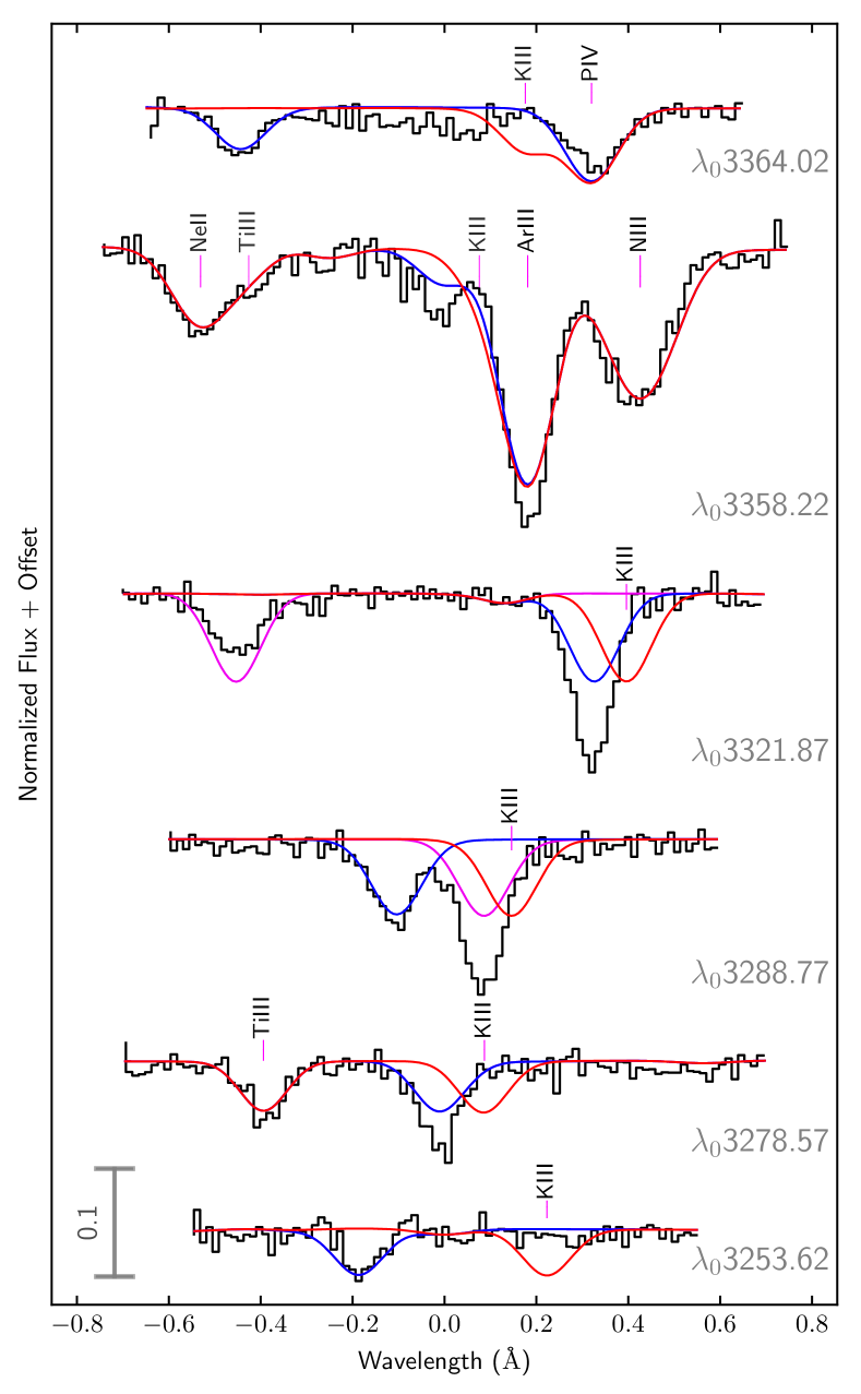
Figure 5: The strongest K iii lines in the observed spectrum of HZ 44. The model using the Kurucz wavelengths is shown in red, while a model with shifted lines is shown in blue. Alternative line shifts are shown in violet (marked with ^∗ in Table 6). All models have a potassium abundance of $\log\mathrm{K/H}=-5$.

While there are no usable calcium lines in the optical spectrum of HD 127493, HZ 44 shows some strong Ca ii and Ca iii lines. The optical resonance lines Ca ii $\lambda\lambda\,$3934, 3968 Å are almost entirely photospheric. Some strong Ca iii lines were excluded from the fit (e. g. Ca iii $\lambda\lambda\,$3372.68, 3537.78 Å) since they have sharp cores and are too broad and shallow in the model. Non-LTE effects can not be blamed since we included Ca ii and Ca iii in non-LTE. We measure $\log\mathrm{Ca/H}=-3.9\pm 0.24$ (28 times solar) for HZ 44 and derive an upper limit of $\log\mathrm{Ca/H}\leq-3.9\pm 0.2$ (12 times solar) for HD 127493. This upper limit is likely to be close to the actual abundance since including Ca at this abundance improves the fit for blended UV lines such as Ca iii 1545.30 Å and Ca iv $\lambda\lambda$ 1647.44, 1648.62, 1655.53 Å.
The strongest titanium iii-iv lines lie in the UVA spectral region although some lines exist at longer wavelengths. We measure a strong enrichment in HZ 44 with $\log\mathrm{Ti/H}=-4.56\pm 0.22$ (150 times solar). This abundance is consistent between strong optical and ultraviolet lines (e. g. Ti iv $\lambda\lambda$ 1183.63, 1451.74, 1467.34, 1469.19 Å and Ti iii 1498.70 Å). Although Ti lines at wavelengths above 3800 Å are strong in HZ 44, the same lines are weak in HD 127493. The few lines that can clearly be identified in HD 127493 (Ti iv $\lambda\lambda\,$4397.31, 5885.97 Å) do not give a consistent abundance. Other predicted lines (Ti iv $\lambda\lambda\,$4397.31, 5398.93, 5492.51 Å) are not observed. Therefore we adopt a conservative upper limit of $\log\mathrm{Ti/H}\leq-4.40\pm 0.25$ (94 times solar) for HD 127493 based on optical lines. However, Ti iii-iv lines in the IUE range would favor higher abundances.

6.3 Fe and Ni (NLTE)

We determine iron abundances by fitting the IUE spectrum of HZ 44 and the GHRS spectrum of HD 127493 in ranges that span 10 to 20 Å, from 1300 Å onward (at shorter wavelengths, the amount of unidentified opacity increases). Since Fe and Ni were fitted separately, blends are not treated exactly which may lead to overestimated abundances. However, since abundances in the initial model were already close to the best-fit abundances, this effect is partly compensated. Missing opacity from other sources may also introduce a bias toward higher abundances but since the observed spectrum is well-reproduced in the considered ranges, we are confident that the derived abundances are reliable within their respective uncertainties. The average of the abundances over all ranges yields $\log\mathrm{Fe/H}=-4.00\pm 0.25$ (1.5 times solar) for HZ 44  and $\log\mathrm{Fe/H}=-2.82\pm 0.13$ (10 times solar) for HD 127493.
The same procedure was applied for nickel, resulting in $\log\mathrm{Ni/H}=-4.05\pm 0.15$ (26 times solar) for HZ 44 and $\log\mathrm{Ni/H}=-3.61\pm 0.13$ (31 times solar) for HD 127493.

6.4 Additional iron-group abundances (LTE)

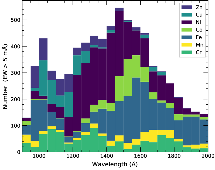
Figure 6: Histogram of iron-peak lines with estimated equivalent widths larger than 5 mÅ in the final model of HZ44. Bins are every 50 Å. Elements are listed in the legend in the same order as they appear in the histogram.

The UV spectral range is dominated by lines from iron-peak elements. Although most lines are from iron and nickel, opacity contributions from other iron-peak elements are also significant. Figure 6 shows the number of lines from iron-peak elements with estimated equivalent width larger than 5 mÅ in the final model for HZ 44. While many of these lines are observed in FUSE and IUE spectra, the opacity peak below 900Å is outside of our observed spectral range.
Our models include only Fe and Ni in non-LTE.
Many vanadium lines in the IUE spectrum of HZ 44 would fit well with abundances of up to $\log\mathrm{V/H}=-4.8$ (e. g. V iv $\lambda\lambda\,$1226.53, 1308.05, 1356.53, 1426.65, 1520.16, 1522.51, 1810.58, 1817.69, 1861.57 Å, and V v 1680.20 Å). It seems unlikely that such a large amount of lines would fit the observation due to accidental alignment with unmodeled blends. However, other lines suggest abundances below $\log\mathrm{V/H}\leq-6.0\pm 0.4$, e. g. V iv $\lambda\lambda\,$1317.56, 1329.28, 1355.13, 1806.20 Å. Several lines in the FUSE spectrum seem to exclude abundances of more than $\log\mathrm{V/H}\leq-5.2\pm 0.4$, e. g. V iv $\lambda\lambda\,$1071.06, 1112.20, 1123.43 Å, and V iii 1149.95 Å, although they lie in regions where the continuum is poorly defined. We conclude that a precise abundance determination for vanadium would require a more complete model, possibly including V in non-LTE. Alternatively, it is possible that some V oscillator strengths are uncertain. Therefore we set an upper limit of $\log\mathrm{V/H}\leq-4.8\pm 0.4$ (893 times solar) for HZ 44. As for HD 127493, V iv $\lambda\lambda\,$1317.56, 1329.28 Å seem to exclude abundances higher than $\log\mathrm{V/H}\leq-6.0\pm 0.4$ (25 times solar). However, these lines may not be reliable since the also give a low upper limit in HZ 44. We therefore adopt no upper limit for HD 127493.
Chromium shows many strong lines in the ultraviolet spectrum of both stars, e. g. Cr iv $\lambda\lambda\,$1433.89, 1658.08, 1825.00, 1826.22, 1826.88, 1827.43 Å. The overall fit is good and we adopt an abundance of $\log\mathrm{Cr/H}=-4.4\pm 0.3$ (28 times solar) for HZ 44 and $\log\mathrm{Cr/H}=-3.9\pm 0.3$ (76 times solar) for HD 127493.
We derive the manganese abundance in HZ 44 from FUSE and IUE to be $\log\mathrm{Mn/H}=-4.9\pm 0.4$ (22 times solar). Fairly strong and unblended lines are, among many others: Mn iii $\lambda\lambda\,$917.80, 956.47 Å and Mn iv $\lambda\lambda\,$1450.36, 1780.00, 1786.05 Å. For HD 127493  we derive an upper limit of $\log\mathrm{Mn/H}\leq-5.5\pm 0.3$ (2.5 times solar) from several undetected lines in the GHRS spectrum such as Mn iv $\lambda\lambda\,$1244.33, 1720.87, 1721.49, 1724.90 Å.
Cobalt lines in the FUSE spectrum of HZ 44 (e. g. Co iii $\lambda\lambda$ 944.77, 946.54, 946.61 Å) suggest an upper limit of $\log\mathrm{Co/H}\leq-5.6\pm 0.4$. Many Co lines in the IUE region, e. g. Co iv $\lambda\lambda\,$1451.43, 1502.06, 1502.70, 1508.42 Å support this upper limit. Other lines fit well with this upper limit or a slightly higher abundance: Co iv $\lambda\lambda\,$1494.75, 1500.58, 1502.19, 1565.91 Å. Because of the unambiguous identification of Co lines and the slight discrepancy between upper limit and best-fit we adopt $\log\mathrm{Co/H}=-5.6\pm 0.5$ (12 times solar) with a relatively large uncertainty. In HD 127493, Co iv $\lambda\lambda\,$1535.28, 1540.56, 1548.83, 1559.64, 1636.40 Å are resolved by GHRS and fit well with an abundance of $\log\mathrm{Co/H}=-5.1$, while Co iv $\lambda\lambda\,$1415.05, 1550.28, 1562.06 Å suggest an abundance no higher than $\log\mathrm{Co/H}\leq-5.3$. We therefore adopt an abundance of $\log\mathrm{Co/H}=-5.3\pm 0.3$ (9 times solar) and note that discrepancies between single lines could result from inaccuracy in line wavelengths or non-LTE effects.
Many strong copper lines lie in the FUV spectral region. Cu iv $\lambda\lambda\,$1053.73, 1057.62 Å in the FUSE spectrum of HZ 44 are quite strong and almost free from blends. Other strong Cu lines are affected by unidentified blends or lie in a region where the continuum placement is not well constrained. Cu lines are weaker in the IUE spectrum, with a few notable exceptions: Cu iii $\lambda\lambda\,$1674.59, 1684.63, 1702.11 1709.03, 1722.37 Å. We determine an abundance of $\log\mathrm{Cu/H}=-5.8\pm 0.4$ (49 times solar) from the lines listed above. Cu v lines such as Cu v $\lambda\lambda\,$1245.99, 1255.30, 1268.32, 1274.74, 1286.55, 1299.16 Å in the GHRS spectrum of HD 127493 exclude abundances higher than $\log\mathrm{Cu/H}\leq-6.1\pm 0.4$ (11 times solar).
The zinc abundances in HZ 44 and HD 127493 are based on strong Zn iii-iv lines that lie mostly in the IUE spectral range. Zn iv is the dominant ion in HD 127493 while HZ 44 shows about the same amount of Zn iii and Zn iv lines. We derive $\log\mathrm{Zn/H}=-5.7\pm 0.3$ (26 times solar) for HZ 44 and $\log\mathrm{Zn/H}=-5.3\pm 0.3$ (29 times solar) for HD 127493.

6.5 Detected trans-iron peak elements (LTE)

We were able to measure the abundance of Ge, Ga, and Pb based on their UV lines in both HZ 44 and HD 127493. In HZ 44 we could additionally derive abundances for As and Sn based on the FUSE spectrum.
In the following we will give a brief overview of the atomic data and lines used for the abundance measurement of each element. The uncertainties on the abundances can be quite large. This can be the result of strong blending with unidentified lines, of the sparse atomic data available for most of these elements, and potential non-LTE effects. Even if atomic data are available, oscillator strengths and line wavelengths are not always well tested.
We use data from TOSS for gallium iv-v and data from O’Reilly & Dunne (1998) for Ga iii with updates for two lines from Nielsen et al. (2005). Many Ga lines are observed in the UV spectra of HZ 44 and HD 127493. The strongest, isolated lines in HZ 44 include Ga iv $\lambda\lambda$ 1163.609, 1170.585, 1258.801, 1299.476, 1303.540, and 1347.083 Å. However, a precise abundance measurement is difficult since most lines are relatively weak and blended with lines from other elements. Nevertheless, we measured an abundance of $\log\mathrm{Ga/H}=-6.0\pm 0.5$ (440 times solar) for HZ 44. We only derive an upper limit of $\log\mathrm{Ga/H}\leq-6.4\pm 0.4$ (80 times solar) for HD 127493 since all Ga lines are weaker and blended.

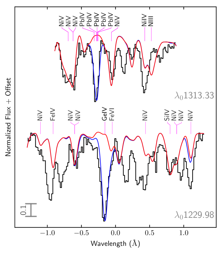
Figure 7: Ge iv and Pb iv lines in the GHRS spectrum of HD 127493. In blue: a model with $\log\mathrm{Ge/H}=-5.0$, $\log\mathrm{Pb/H}=-5.7$. In red: the same model without Pb and Ge.

Germanium shows many lines in the FUSE and IUE spectral range, including the strong resonance lines Ge iv $\lambda\lambda$ 1189.028, 1229.840 Å and Ge iii 1088.463 Å. We identified lines from Ge iii-v in HZ 44 which can be matched at an abundance of $\log\mathrm{Ge/H}=-5.9\pm 0.3$. (140 times solar). For HD 127493, we derive an abundance of $\log\mathrm{Ge/H}=-5.0\pm 0.4$ (470 times solar) from the strong resonance lines Ge iv 1189.028 Å (IUE) and Ge iv 1229.840 Å (GHRS, shown in Fig. 7).
Morton (2000) lists oscillator strengths for ten ultraviolet arsenic iii lines from low-lying levels, as computed by Marcinek & Migdalek (1993). Oscillator strengths for several optical As iv lines are listed in ALL, originally from Churilov & Joshi (1996). The only ultraviolet As iv line listed in Morton (2000) is the resonance line As iv 1299.28 Å but the oscillator strength provided by Curtis (1992) is low ($f=1.94\cdot 10^{-3}$). Atomic data for the two resonance lines As v 987.651 Å and As v 1029.480 Å is provided by Pinnington et al. (1981), as listed in Morton (2000). These As v oscillator strengths have previously been used for the As abundance measurement in DO white dwarfs by Chayer et al. (2015) and Rauch et al. (2016a). Morton (2000) also lists a third resonance line, As v 1001.211 Å. This line is not observed in the spectrum of HZ 44 and was disregarded by both Chayer et al. (2015) and Rauch et al. (2016a). It is only mentioned in Froese Fischer (1977) (and may have been confused with the ²S${}_{1/2}-^{2}$P_1/2 transition line As v 1029.480 Å). Neither NIST (Moore, 1971) nor Joshi & van Kleef (1986) list an energy level that would be consistent with an As v resonance line at 1001.211 Å, so we decided to exclude it as well. As iii lines are weak in HZ 44 and As iii $\lambda\lambda$ 927.540, 944.726 Å exclude abundances higher than $\log\mathrm{As/H}\leq-6.4\pm 0.4$ (960 times solar). As iv 1299.28 Å would fit an otherwise unidentified line at an abundance of $\log\mathrm{As/H}=-5.6$ which is excluded by other lines. Figure 8 shows the strongest observed As lines in HZ 44, As v 987.651 Å and As v 1029.480 Å. We use these lines to derive an abundance of $\log\mathrm{As/H}=-7.4\pm 0.4$ (100 times solar). As iv 1299.28 Å is also visible in the GHRS spectrum of HD 127493 and fits the observation at an abundance of $\log\mathrm{As/H}=-4.9\pm 0.4$ (1300 times solar). Due to the discrepancy observed in HZ 44, we do not consider this an abundance measurement.
Also as part of their “Stellar Laboratories” series Rauch et al. (2017b) have measured the abundance of selenium in the peculiar DO white dwarf RE 0503$-$289. We use their oscillator strengths for Se v and results from Bahr et al. (1982) for Se iv, as listed in Morton (2000). Se iv $\lambda\lambda\,$ 959.590, 996.710 Å and Se v 1094.691 Å fit strong, otherwise unidentified lines at $\log\mathrm{Se/H}=-6.3\pm 0.6$. However, Se iv 984.341 Å seems to exclude abundances higher than $\log\mathrm{Se/H}\leq-7.6\pm 0.4$. Like As v 1001.211 Å this line may not be real; its lower level is not listed in NIST nor in the newest reference on Se iv energy levels we found, Pakalka et al. (2018). Therefore, we adopt an abundance of $\log\mathrm{Se/H}=-6.3\pm 0.6$ (110 times solar) for HZ 44.

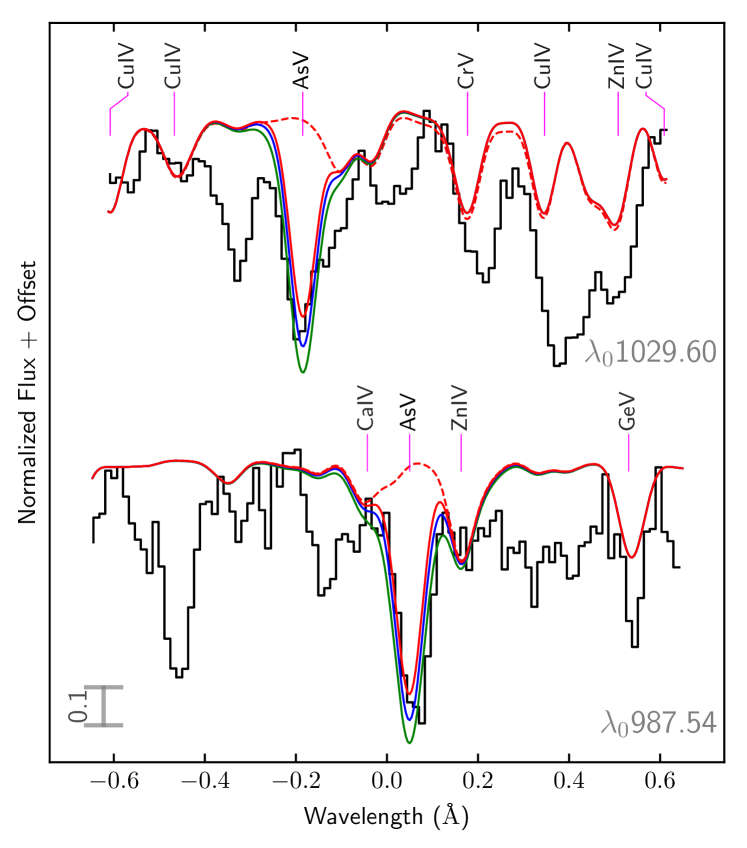
Figure 8: As v 987.651 Å and As v 1029.480 Å in the FUSE spectrum of HZ 44. In red: a model with $\log\mathrm{As/H}=-7.8$; dashed without As. In blue: the adopted abundance $\log\mathrm{As/H}=-7.4$. In green: $\log\mathrm{As/H}=-7.0$.

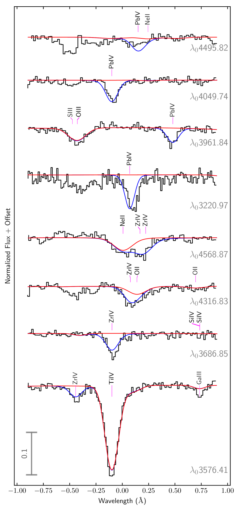
Figure 9: A selection of Zr iv and Pb iv lines in the HIRES spectrum of HZ 44. In blue: a model with $\log\mathrm{Zr/H}=-5.9$ and $\log\mathrm{Pb/H}=-5.9$. In red: the same model, but without Zr or Pb.

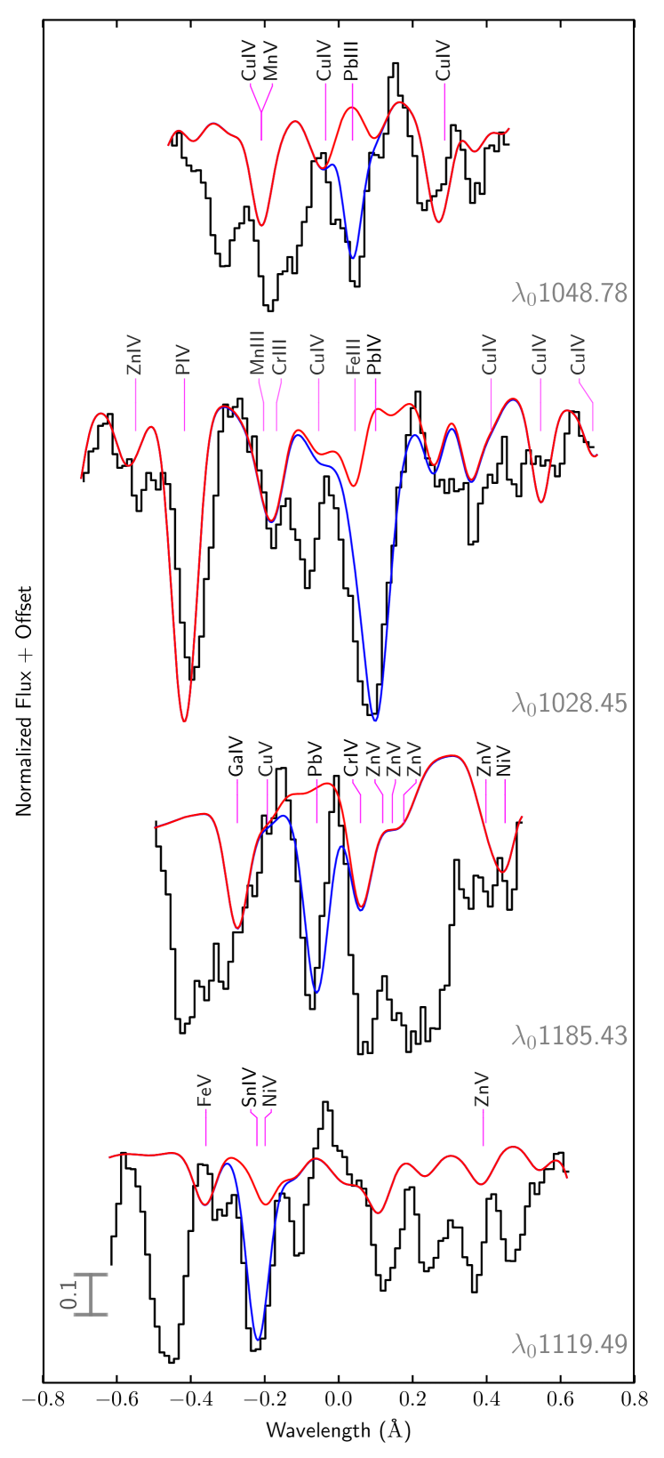
Figure 10: Pb iii, Pb iv, Pb v, and Sn iv lines in the FUSE spectrum of HZ 44. In blue: a model with $\log\mathrm{Pb/H}=-5.9$ and $\log\mathrm{Sn/H}=-6.9$. In red: the same model without Pb and Sn.

HZ 44 is one of the very few hot subdwarf stars showing zirconium in its optical spectrum. We used the atomic data from Rauch et al. (2017a) for our analysis. We fitted four distinct Zr iv lines in the HIRES spectrum of HZ 44 (Zr iv $\lambda\lambda\,$ 3576.107, 3686.902, 4317.077, 4569.218, 4569.272 Å, see Fig. 9) and found an abundance of $\log\mathrm{Zr/H}=-5.92\pm 0.19$ (1500 times solar). The UV spectra of HZ 44 also show Zr iv-v lines, and although none of them are strong or isolated enough to independently measure the abundance, they are consistent with abundance derived from the optical lines. The doublet Zr iv $\lambda\lambda$ 4569.218, 4569.272 Å is visible in HD 127493 and would fit well with an abundance of $\log\mathrm{Zr/H}=-5.5$ (1700 times solar). Since no other lines could clearly be identified as Zr we adopt an upper limit of $\log\mathrm{Zr/H}\leq-5.4\pm 0.2$.
Tin is one of the elements that were identified in HZ 44 by O’Toole (2004). We used atomic data from Safronova et al. (2003), supplemented with data from Biswas et al. (2018) for Sn iv and results from Haris & Tauheed (2012) for Sn iii. We derived the Sn abundance in HZ 44 to be $\log\mathrm{Sn/H}=-6.9\pm 0.4$ (550 times solar), based on the strong Sn iv 1119.338 Å line which is almost free from blends (see Fig. 10). The other strong, but blended Sn iv $\lambda\lambda$ 1019.720, 1044.487, 1314.539 Å, and Sn iv 1437.527 Å (blended with Co iv 1437.488 Å) lines support this measurement. Even if the FUSE continuum is estimated too high in our models, Sn lines in the IUE spectrum, where the model is more complete, set the upper limit to $\log\mathrm{Sn/H}\leq-6.5\pm 0.4$ (1400 times solar). Sn iv 1314.539 Å excludes abundances higher than $\log\mathrm{Sn/H}\leq-6.6\pm 0.4$ (480 times solar) for HD 127493.
We collected atomic data for lead iii-v from several sources. Pb iii oscillator strengths are from Alonso-Medina et al. (2009), with the exception of the resonance lines Pb iii 1048.877 Å and Pb iii 1553.021 Å which are based on lifetime measurements by Ansbacher et al. (1988) as listed in Morton (2000). For Pb iv, we use oscillator strengths from Safronova & Johnson (2004) with additional lines from Alonso-Medina et al. (2011) and one line (Pb iv 4496.15 Å) from Naslim et al. (2013). Data for Pb v is provided by Colón et al. (2014). While this collection is far from complete, many Pb lines could be identified, including not only strong Pb iii-v lines in the ultraviolet spectrum of HZ 44 but also five Pb iv lines in its optical spectrum (Pb iv $\lambda\lambda$ 3052.56, 3221.17, 3962.48, 4049.80, 4496.15 Å, see Fig. 9).

Fitting all identified Pb lines in the HIRES spectrum except Pb iv 3052.56 Å (S/N too low) results in $\log\mathrm{Pb/H}=-5.89\pm 0.09$ (11000 times solar). This is remarkably consistent with Pb lines observed in the UV region, including lines from Pb iii and Pb v. As far as we know, this is the first time Pb v lines were modeled in any star. The strongest Pb lines per ionization stage observed in the FUSE spectrum of HZ 44 are shown in Fig. 10. The Pb abundance measurement in HD 127493 is based mostly on Pb iv 1313 Å (see Fig. 7), assuming a solar isotopic ratio as in O’Toole & Heber (2006). We derive an abundance of $\log\mathrm{Pb/H}=-5.65\pm 0.40$ (8400 times solar), consistent with Pb v $\lambda\lambda$ 1233.50, 1248.46 Å in the GHRS spectrum.

6.6 Trans-iron elements with upper limits

The abundance measurements for Se, Kr, Sr, Y, Mo, Sb, Te, Xe, and Th turned out to be inconclusive because too few lines were found and/or their relative line strengths were at variance with model predictions. Instead we derived upper limits for these elements.
Krypton and strontium belong to the group of elements that have been studied in white dwarfs by Rauch et al. (2016b, 2017b). Despite the large number of Kr iv-v lines in the TOSS line list, none of them are strong enough in the final synthetic spectrum of HZ 44 to be identified in the observation. We derive an upper limit of $\log\mathrm{Kr/H}\leq-5.2\pm 0.6$ (1700 times solar) from four undetected Kr iv lines, the strongest being Kr iv 1538.211 Å. Kr iv 999.388 Å would fit well with an abundance of $\log\mathrm{Kr/H}=-5$ but is likely blended. Kr iv $\lambda\lambda$ 1400.898, 1538.211, 1558.514 Å and Kr v 1293.917 Å in GHRS spectrum of HD 127493 exclude abundances higher than $\log\mathrm{Kr/H}\leq-4.8\pm 0.4$ (1900 times solar).
The situation is similar for strontium in HZ 44. The undetected Sr v 962.378 Å, Sr iv 1244.137 Å, and Sr iv 1244.763 Å lines exclude abundances higher than $\log\mathrm{Sr/H}\leq-5.1\pm 0.6$ (5100 times solar). Sr iv 1331.129 Å would fit well with $\log\mathrm{Sr/H}=-5.0$. Sr iv $\lambda\lambda$ 1244.137, 1244.888, 1268.622, 1275.354, 1729.533 Å in GHRS exclude abundances higher than $\log\mathrm{Sr/H}\leq-4.9\pm 0.3$ (3600 times solar) in HD 127493.
Naslim et al. (2011) have observed yttrium in the iHe hot subdwarf LS IV$-14^{\circ}116$. So far it has been observed to be extremely enriched in two additional iHe-sds: HE 2359$-$2844 (Naslim et al., 2013) and [CW83] 0825$+$15 (Jeffery et al., 2017). We used their oscillator strengths for Y iii 4039.602 Å and Y iii 4040.112 Å to search for Y in HZ 44 and HD 127493. Both lines are predicted to be weak in the models and were not detected in the spectra of either star. We derive an upper limit of $\log\mathrm{Y/H}\leq-5.3\pm 0.2$ (14800 times solar) for HZ 44. Due to the lower S/N of the FEROS spectrum and the higher temperature in HD 127493, the upper limit derived from the same lines in that star is even higher: $\log\mathrm{Y/H}\leq-4.7\pm 0.3$ (26000 times solar). None of the ultraviolet Y iii lines for which Redfors (1991) computed oscillator strengths are strong enough to improve on this threshold. Unfortunately, we found no oscillator strength measurements for the resonance lines Y iii 1000.563 Å and Y iii 1006.587 Å that are listed in Morton (2000). A more complete analysis of Y in subdwarf stars would benefit from oscillator strengths for Y iv which is the dominant ionization stage at effective temperatures around 40 000 K.
Rauch et al. (2016a) have observed molybdenum in RE 0503$-$289. We use their atomic data for Mo v and atomic data from the Kurucz line list for Mo iv to search for Mo in HZ 44. Mo iv $\lambda\lambda\,$965.485, 966.638 Å and Mo v $\lambda\lambda\,$939.248, 1127.101 Å are well reproduced with $\log\mathrm{Mo/H}=-6.4$ (2500 times solar). Since these lines are relatively weak and our model is missing opacity in the FUSE region, we adopt an upper limit of $\log\mathrm{Mo/H}\leq-6.2\pm 0.4$ (4000 times solar). Several lines in the IUE spectrum return a non-detection compatible with this upper limit, for example Mo v $\lambda\lambda\,$ 1586.898, 1774.317 Å. As for HD 127493  Mo v $\lambda\lambda\,$ 1586.898, 1590.414, 1653.541 1661.215 1774.317 Å exclude abundances higher than $\log\mathrm{Mo/H}\leq-6.1\pm 0.4$ (2200 times solar).
Werner et al. (2018) have recently measured photospheric abundances of antimony in two DO white dwarfs: RE 0503$-$289 and PG 0109+111. Both stars are chemically peculiar, with strong enrichment of trans-iron elements. Despite blends with unidentified lines in FUSE and the low resolution of IUE, we were able to set the upper limit on the Sb abundance in HZ 44 to $\log\mathrm{Sb/H}\leq-8.0\pm 0.5$ (470 times solar), which is well below the extreme enrichment observed in the two aforementioned white dwarfs. This upper limit is based on three lines: Sb iv 1042.190 Å (blended with Cr iv), Sb v 1104.23 Å, and Sb v 1226.001 Å. Sb v 1104.23 Å even fits well at this abundance.

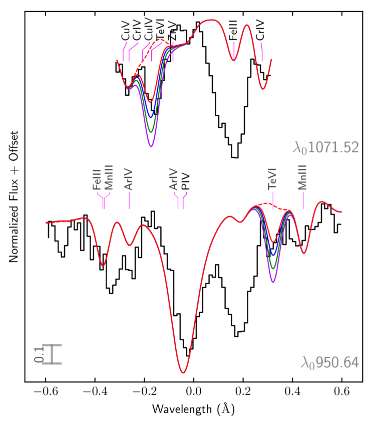
Figure 11: Te vi resonance lines in the FUSE spectrum of HZ 44. We show a model with $\log\mathrm{Te/H}=-7.9$ (red) and without Te (dashed). Models including higher Te abundances are further shown: $\log\mathrm{Te/H}=-7.5$ (blue), $\log\mathrm{Te/H}=-7.1$ (green), and $\log\mathrm{Te/H}=-6.7$ (pink).

Zhang et al. (2013) have computed oscillator strengths for tellurium ii-iii, including UV and optical lines. However, since the Te iii population numbers are low in HZ 44, none of these lines are visible. Rauch et al. (2017b) provided oscillator strengths for Te vi lines, including the resonance lines Te vi $\lambda\lambda$ 951.021, 1071.414 Å, which are visible in HZ 44 (see Fig. 11). They are best reproduced with an abundance of $\log\mathrm{Te/H}=-7.5\pm 0.4$ (100 times solar). Due to the weakness of the lines and their position in the FUSE spectrum we only adopt an upper limit of $\log\mathrm{Te/H}=-7.1\pm 0.4$ (250 times solar). The Te v 1281.670 Å resonance line listed in Morton (2000); Pinnington et al. (1985b) also supports this upper limit. Te v 1281.670 Å is also visible in the GHRS spectrum of HD 127493, but blended with a weaker Co v line. We derive an upper limit of $\log\mathrm{Te/H}=-5.8\pm 0.4$ (2200 times solar).
We use oscillator strengths for xenon iv-v from Rauch et al. (2017a) provided on the TOSS website in order to look for Xe in HZ 44. Most Xe lines in the FUSE spectrum of HZ 44 are blended with unidentified lines. The resonance lines Xe iv $\lambda\lambda$ 935.251, 1003.373 Å and Xe v $\lambda\lambda$ 936.284, 945.248 Å allow us to set an upper limit of $\log\mathrm{Xe/H}\leq-7.3\pm 0.4$ (140 times solar). The actual Xe abundance in HZ 44 might be close to our upper limit, since the additional opacity improves the fit for many lines. However, the only isolated line that could be identified is Xe v 936.284 Å.
Thorium is the heaviest element for which we found atomic data. It is of particular interest since it is not produced through the s-process and can be used for age determination because of its radioactivity. Safronova & Safronova (2013) have computed atomic properties of 24 low-lying states of the Th iv ion. Atomic data for Th iii are published in Safronova et al. (2014), but could not be used here since all transitions with calculated oscillator strengths lie in the infrared region. Even with a relatively low abundance of $\log\mathrm{Th/H}=-8.5$ (1400 times solar), our models predict several Th iv lines with estimated equivalent widths up to 30 mÅ in the UV range. In particular, the non-detection of Th iv 983.140 Å (which falls conveniently on one of the few points of pseudo-continuum in the FUSE spectrum of HZ 44), Th iv 1140.612 Å (in the wing of a well-modeled Si iii line), and Th iv 1682.213 Å allow us to set the upper limit for the photospheric Th abundance in HZ 44 to $\log\mathrm{Th/H}\leq-8.0$ (4600 times solar). We derive an upper limit of $\log\mathrm{Th/H}\leq-7.8\pm 0.3$ (3200 times solar) for HD 127493 based on the Th iv $\lambda\lambda$ 4413.576, 5420.380, 5841.397, 6019.151 Å lines in the FEROS spectrum.

6.7 An unsuccessful search for additional trans-iron elements

We also searched for predicted lines of Sc, In, Ba, Tl, and Bi in the ultraviolet and optical spectra of HZ 44. However, no lines from these elements could be identified and no meaningful upper limit could be derived either.
The strongest scandium lines in the model of HZ 44 are the resonance line Sc iii 1610.194 Å and Sc iii 1603.064 Å. Both lines are weak in the model, even at a high abundance of $-5$ dex relative to hydrogen and are blended with both modeled and unidentified lines, so no meaningful upper limit could be determined.
Safronova et al. (2003) have calculated atomic properties along the silver isoelectronic sequence, including In iii, Sn iv, and Sb v. They predict indium iii lines from low-lying levels with high oscillator strengths in the IUE spectral region. However, the population numbers for In iii are too low to set a meaningful upper limit for both HZ 44 and HD 127493.
Barium was observed in RE 0503$-$289 by Rauch et al. (2014) who also provide atomic data for Ba v. The predicted Ba v lines are so weak in the model of HZ 44 that $\log\mathrm{Ba/H}=-5$ (32000 times solar) is required before the strongest predicted lines in synthetic spectrum of HZ 44 (Ba v $\lambda\lambda\,$1097.415, 1103.140 Å) reach equivalent widths of 0.1 mÅ. It was therefore not possible to set a meaningful upper limit.
The strongest observable bismuth line in the spectrum of HZ 44 is by far Bi v 1139.549 Å. Since it is blended with an unidentified line, we can only derive an upper limit of $\log\mathrm{Bi/H}\leq-8.5$ (340 times solar). We consider this upper limit preliminary since it is based on a single, blended line in the FUSE spectrum.
Oscillator strengths along the gold isoelectronic sequence were computed by Safronova & Johnson (2004), including not only Pb iv but also thallium iii. Similar to In iii, the population number for Tl iii is too low to set a meaningful upper limit in both HZ 44 and HD 127493.

6.8 Chemical composition summary

Figures 12 and 13 as well as Table 11 show our final abundance values for HZ 44 and HD 127493. The abundance patterns are remarkably similar in both stars despite the $\sim$2500 K difference in their effective temperature. The overall resemblance between the chemistry of both stars is especially visible when comparing their abundances in number fractions (Fig 13). In addition, some trans-iron elements are present in the atmosphere with very similar abundances. For example, in HZ 44 Cu, Zn, Ga, Ge, Zr, and Pb have the same number fraction of $\sim 10^{-6.2}$, whereas the solar abundances show a strong decrease with increasing atomic mass. As and Sn are significantly less abundant than the other trans-iron elements.
Both stars show a strong CNO cycle pattern, most obvious in Fig. 13, with nitrogen being enriched while carbon and oxygen are depleted with respect to solar values. Ne is mildly enriched (by a factor of 3) in both stars compared to solar. With the exception of Cl, all elements with $11\leq\mathrm{Z}\leq 20$ are more abundant in HZ 44 than in the Sun. The abundance of Mg, Al, Si, and S is similar in both stars. With a measured abundance of $148^{+98}_{-61}$ times solar, the Ti iv lines are very strong in the UVA spectrum of HZ 44. In contrast, the Ti lines covered by the FEROS spectrum of HD 127493 are weak and set an upper limit for Ti to $94^{+105}$ times solar. Co and Ni have very similar abundances in both stars: they are about 30 times the solar values. Mn and Cu could not be detected in HD 127493, which indicated that they are less abundant than in HZ 44. As seen in many other hot subdwarf stars, Fe is the least enriched element among the iron group in HZ 44 ($\sim$1.5 times solar). Fe is more enriched ($\sim$10 times solar) in HD 127493. The Zn abundance in both stars is similar to that of Ni, between 25 and 30 times solar. While the Ge abundances in HD 127493 ($\sim$470 times solar) and HZ 44 ($\sim$140 times solar) are similar considering uncertainties, the Ga abundance in HD 127493 ($\lesssim$ 75 times solar) is lower than in HZ 44 ($\sim$440 times solar). The As abundance exceeds that of the Sun by a factor of about 100 in HZ 44. Interestingly, HZ 44 is one of the few hot subdwarf stars showing Zr iv and Pb iv lines in their optical spectrum. As far as we know Zr iv has been identified in the optical spectrum of only two iHe hot subdwarfs, LS IV$-$14^∘ 116 and HE 2359-2844 (Naslim et al., 2011, 2013). Zr is enriched at about 1500 times solar in HZ 44, which is not excluded also in HD 127493. Interestingly, the measured Pb abundance in both stars is almost identical; they are enhanced by a factor of 10000. The enrichment is significantly lower for other heavy elements in HZ 44. In particular Xe and Te exceed the solar abundance by a factor of less than 500 in HZ 44.

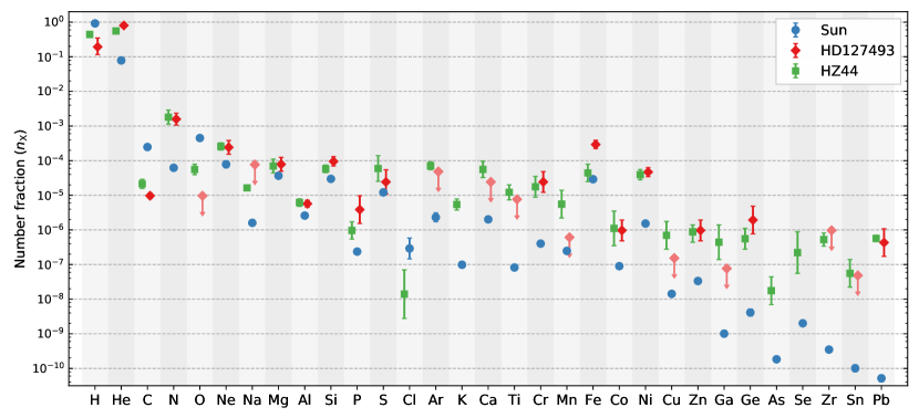
Figure 12: Abundance patterns of HD 127493 and HZ 44 compared to that of the Sun (by number fraction). Only elements with an abundance measurement in at least one of the star are shown. Upper limits are marked with an arrow and less saturated colors.

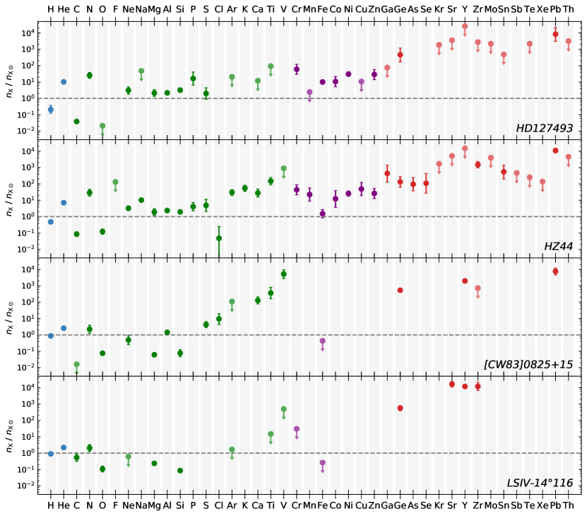
Figure 13: Abundance pattern of HD 127493 and HZ 44 with respect to solar composition. Results for the heavy-metal subdwarfs [CW83] 0825+15 (Jeffery et al., 2017) and LS IV$-14^{\circ}116$ (Naslim et al., 2011) are shown for comparison. Light elements ($23\leq\mathrm{Z}$) are marked by green symbols, iron-peak elements ($24\leq\mathrm{Z}\leq 30$) in purple, and heavier elements ($\mathrm{Z}\geq 31$) in red. Upper limits are marked with an arrow and less saturated colors.

7 Discussion

The Carnegie Yearbook No. 55, for 1955/56 reports the discovery of a new sdO star, BD+25${}^{\circ}4655$, to be similar to HD 127493 and HZ 44 and quotes a very foresighted conclusion (probably by Muench): that the spectrum of the newly discovered sdO “is extremely rich in faint sharp lines, those of N ii, N iii, and Ne ii being especially conspicious. The complete absence of lines of oxygen and carbon, in any stage of ionization, suggests that the surface material of this kind of star has undergone nuclear processes which transformed the carbon into nitrogen and the oxygen to neon.” The abundance of those elements derived in previous quantitative spectral analyses as well as in ours substantiate this statement. The strong overabundances of heavy elements found for HZ 44, HD 127493, and a few other iHe hot subdwarfs stars are generally believed to be caused by atmospheric diffusion processes (radiative levitation). However, it is not plausible to assume that diffusion creates an abundance pattern of C, N, O, and Ne, that mimics the nucleosynthesis pattern so well. In the following subsections, we first discuss the evidence for diffusion processes and compare the abundance patterns of our two stars to that of other iHe hot subdwarfs. Then we revisit the nuclear synthesis aspect and discuss implications for the evolutionary status.

7.1 Diffusion

Diffusion refers to the equilibrium between gravitational settling and radiative levitation. While heavy elements are pulled downwards by gravity, their important line opacities in the UV region, where the photospheric flux distribution peaks, lead to opposing forces due to radiation pressure. This force is limited by the saturation of spectral lines at high abundances. Once an equilibrium of both forces has been established, the elemental abundances should be fixed.
Models that account for gravitational settling and radiative levitation only fail to reproduce the observed abundances pattern of sdB stars (see Heber, 2016, for a discussion). Additional processes have to be taken into account. Stellar winds and turbulent mixing have been suggested. Michaud et al. (2011) have studied the effects of non-equilibrium diffusion and radiative levitation on element abundances up to Ni for sdB stars on the horizontal branch (up to $T_{\mathrm{eff}}\approx 37\,000$ K), but not for sdOs. To match the iron abundances observed in sdBs by Geier et al. (2010), and later Geier (2013), they required some process to dampen the effect of radiative levitation. Michaud et al. (2011) adopted a turbulent surface mixing zone during the HB evolution that includes the outer $\sim$ $10^{-7.5}\,\mathrm{M}_{\odot}$ in the envelope. Similarly to the sdOs discussed in this paper, the photospheric iron abundance in sdBs is approximately solar. This low Fe enhancement is a result of its high absolute abundance in the photosphere and the consequent line saturation (see Fig. 12). Since heavy elements, such as Zr and Pb, are initially less abundant in absolute terms, a stronger enrichment due to radiative levitation is expected. The models for the hottest stars ($T_{\mathrm{eff}}$ = 35$-$37 kK) in Michaud et al. (2011) predict abundances that are lower than what is observed in HZ 44 and HD 127493. For example, N, Ne, Al, Si, and Mg are predicted to be depleted with respect to the solar values. Thus additional processes are required to explain the abundance pattern of our two sdOs; nucleosynthesis during the formation of the stars, weak stellar winds (Unglaub, 2008; Hu et al., 2011) and a possible atmospheric surface convection zone (Groth et al., 1985; Unglaub, 2010) might well be involved.
The models by Michaud et al. (2011) can not reproduce the He-enrichment and CNO-cycle pattern observed in some sdBs (and the sdOs discussed here) since they use approximated methods to evolve their models through the He-flash. Byrne et al. (2018) have preformed similar calculations for post common envelope sdBs from the top of the RGB to the zero age HB with a more self-consistent treatment of the He-flash. They produced He-rich atmospheres in their delayed He-flash models and predict C and N to be enriched and O to be depleted for sdBs on the zero-age horizontal branch (ZAHB). The abundances of other elements are similar to those of Michaud et al. (2011) but both models are not especially well-suited for the hotter stars discussed here. Detailed sdO evolutionary models (e. g. through the HeWD-merger channel) including diffusion of heavy elements beyond the iron group would be required to explain the observed abundance pattern. Unfortunately, the atomic data required for modeling diffusion of elements heavier than Ni is still lacking.

7.2 Comparison with other iHe hot subdwarfs

In Fig. 13 we compared the abundance pattern of HZ 44 and HD 127493 with literature abundances of two other iHe subdwarf stars: [CW83] 0825$+$15 and LS IV$-14^{\circ}116$.
[CW83] 0825$+$15 is the closest match to HZ 44 and HD 127493 in terms of of atmospheric properties with $T_{\mathrm{eff}}=38\,900$ K and $\log g=5.97$ (Jeffery et al., 2017). Although being less He-rich ($\log\,n_{\mathrm{He}}/n_{\mathrm{H}}=-0.6$), it is the only known heavy-metal iHe hot subdwarf to be C-deficient, like the two stars we analysed here. Its abundance pattern is also similar to HZ 44 and HD 127493 in that the CNO-cycle pattern is evident and lead is equally enriched. However, the abundances of some specific elements differ significantly: Mg and Si are less abundant by $\sim$1 dex while Cl is about 2 dex more abundant in [CW83] 0825$+$15.
LS IV$-14^{\circ}116$ was the first heavy-metal hot subdwarf to be recognized as so and is considered as the prototype of the class, with its extreme enrichment in Sr, Y and Zr (Naslim et al., 2011) With $T_{\mathrm{eff}}=34\,950$ K, $\log g=5.93$, and $\log n_{\mathrm{He}}/n_{\mathrm{H}}=-0.62$ (Green et al., 2011), the star is cooler and less helium-rich than HZ 44 and HD 127493. Similarly to the two other heavy-metal subdwarfs, HE2359-2844 and HE1256-2738, its C abundance is higher than in HZ 44 and HD 127493 (see also Fig. 1). Its Sr and Zr enrichment is stronger than in HZ 44 and HD 127493 (and [CW83] 0825$+$15).
Although the abundances of HZ 44 and HD 127493 are remarkably similar, the patterns observed in other heavy-metal subdwarfs appear to be different. However, it is difficult to draw firm conclusions when abundances are known only for a much more limited subset of elements in the other stars. In the case of LS IV$-14^{\circ}116$ and [CW83] 0825$+$15, the lack of UV data strongly restricts their chemical portrait. Along with [CW83] 0825$+$15, our two stars HZ 44 and HD 127493 are the only known heavy-metal subwarfs to be enriched in nitrogen, but depleted in carbon and oxygen. The three other known heavy metal subdwarfs have higher C-abundances, similarly to the group of CN-rich eHe subdwarfs that is observed at higher temperatures. Whether the differences in the the abundances of carbon and nitrogen in iHe subdwarfs are related to stellar evolution or the effects of diffusion remains unclear.

7.3 Nuclear synthesis and evolutionary status

The formation of hot subdwarfs with intermediate He abundances (10%–90% by number) through merging He-WDs with low-mass MS stars was investigated by Zhang et al. (2017). In these models, subdwarfs with intermediate He-rich atmospheres represent a short ($<5\,$Myr) phase after the He-flash is ignited during the merger. The initially He-rich atmosphere of the merger remnant transforms into a H-rich one as the heavier He diffuses downward (gravitational settling) until the atmosphere is H-rich when the ZAHB is reached. The same process is predicted in accretion-based HeWD+HeWD mergers (Zhang & Jeffery, 2012) that can also reproduce the He abundance in iHe-sds.
A known problem is that merger calculations predict a fast surface rotation. Schwab (2018) has calculated post-HeWD+HeWD merger models with initial conditions taken from hydrodynamic merger calculations and found that merger products have $v_{\mathrm{rot}}\succeq 30$ km s^-1 once they appear as hot subdwarfs. This rotation is usually not observed in single sdBs (Geier & Heber, 2012) and Hirsch (2009) found N-rich He-sdOs (such as HZ 44 and HD 127493) to have $v_{\mathrm{rot}}$ similar to sdBs. For individual stars, this can be explained by a small inclination $i$ (which leads to a small $v_{\mathrm{rot}}\sin i$). However, with increasing evidence for slowly rotating (intermediate) He-sdOs, it seems likely that additional physics is needed to match the observations (Schwab, 2018). Alternatively, slowly rotating hot subdwarfs may be created through a different process altogether.
The observation of the CNO cycle pattern in HD 127493 and HZ 44 indicates that the CNO process must have been efficient in a H-burning shell or mixed from a sufficiently hot core in the stars’ progenitor. In fact, the slow HeWD+HeWD merger model by Zhang & Jeffery (2012) is able to reproduce the CNO pattern observed in HZ 44 and HD 127493 well except for somewhat higher predicted O-abundances. This may be an indication that O has been processed to Ne through the $\alpha$ capture $\isotope[16][8]{O}(\alpha,\gamma)\isotope[20][10]{Ne}$. In HeWD+MS merger models presented by Zhang et al. (2017), temperatures high enough for $\isotope[18][8]{O}(\alpha,\gamma)\isotope[22][10]{Ne}$ burning are reached following the first He-flash, even if the processed material is not always mixed to the surface. That the He, C, N, O, and Ne abundances in some He-sdOs, and in the two stars analysed here, can be explained by nuclear synthesis might indicate that these light elements are less affected by diffusion in this type of stars.
An alternative explanation to diffusion for the extreme enrichment of heavy element could be that they were created in the stars’ progenitor. Heavy elements like Zr and Pb are produced mainly in the s-process, which is thought to be efficient in asymptotic giant branch (AGB) stars. While most hot subdwarfs do not evolve through the AGB phase, low-mass post-AGB tracks are crossing the log $g$ $-T_{\mathrm{eff}}$ diagram in the region populated by luminous hot subdwarfs (Napiwotzki, 2008). Therefore such an evolutionary channel might be responsible for a small fraction of the hot subdwarfs. However, diffusion calculations for these elements are required before conclusions on possible AGB progenitors of heavy-metal enriched iHe-sds can be made.

8 Conclusion

We have performed a detailed spectroscopic analysis of the two intermediate He-sdOs HZ 44 and HD 127493. SED-fits combined with parallax distances for both stars result in masses that are consistent with the canonical subdwarf mass of 0.47 M_⊙ within 1-$\sigma$ uncertainty. No indication of binarity was found for either star. Our main focus was the determination of photospheric metal abundances, including heavy elements. We found the abundance pattern in both stars to be very similar. They show a typical CNO-cycle pattern and slight enrichment of intermediate-mass elements ($\mathrm{Z}\leq 30$, except Cl) compared to solar values. Heavier elements such as Ga, Ge, and As were found to be enriched in the order of 100 times solar. Most interestingly, the abundances of Zr and Pb were measured from optical lines and confirmed with UV transitions in HZ 44, and turned out to be more than 1000 and 10000 times solar, respectively. HD 127493 shows no optical Zr or Pb lines, but we derived a Pb enrichment of about 8000 times solar from Pb iv-v lines in its HST/GHRS UV spectrum. Pb v lines were modeled for the first time in a stellar photosphere and their predicted strength reproduced well the observations of both stars. We also determined upper limits for several additional heavy elements. Some of them, for example Xe and Te, have a moderate enrichment ($\la$ 500 times solar) in HZ 44.
In order to improve the accuracy of abundance measurements, additional atomic data are much-needed, in particular for the heavy elements. Many lines in both the optical and ultra-violet spectra still remain unidentified. This is especially evident in the FUSE spectrum of HZ 44, where not only interstellar but also many photospheric lines are missing from our models. Some of those lines likely belong to ionized heavy elements for which no atomic data, or only a limited subset, are available.
Interestingly, pulsations were observed in three other iHe subdwarfs, namely [CW83] 0825$+$15 (Jeffery et al., 2017), LS IV$-14^{\circ}116$ (Ahmad & Jeffery, 2005), and Feige 46 (Latour et al., 2019). This would make it worth looking for photometric variability in HZ 44 and HD 127493 as well.
As of now, we are not able to fully explain the observed abundance pattern in intermediate He-sdOs. Evolutionary simulations for sdOs including diffusion for heavy elements and mixing during hot flasher/merger evolution would be required to interpret the abundance pattern. Even though we obtained a quite exhaustive chemical portrait for the two stars analysed here, this is generally not the case for the other iHe hot subdwarfs. More complete set of abundances for additional stars are also necessary to properly investigate these intriguing patterns.
The efficiency of radiative support on heavy elements in hot subdwarfs might be linked to their helium abundance, given that the intermediate helium-rich hot subdwarfs seem to favorably display extreme enhancements. Hydrogen-rich sdB stars were found to be enriched in some heavy elements as well (O’Toole & Heber, 2006; Blanchette et al., 2008), but their enrichment in Pb for example is significantly lower than that observed in the heavy-metal iHe subdwarfs. At the other end of the helium abundance spectrum, abundance analyses of He-sdOs are more limited, especially concerning heavy metals. The only He-rich sdO for which heavy metal abundances have been derived, BD+39 3226, turned out the be less than 2 dex enhanced in Zr and Pb (Chayer et al., 2014). It would be most interesting to determine abundances of heavy elements in additional He-rich stars. The He-sdOs recently analyzed by Schindewolf et al. (2018) would be well-suited to confirm (or not) this milder enrichment in heavy metals. Their atmospheric parameters, as well as their abundances of lighter elements are well constrained, and excellent UV data are available. The current set of hot subdwarfs for which abundances of heavy elements are known do not allow us to rule out the possibility that the effective temperature also plays a role in favoring the radiative support of particular elements. Once again abundances for a larger sample of stars across the $T_{\mathrm{eff}}$ range where the extreme overabundances are observed ($\sim$ 34$-$43 kK), also including hydrogen-rich stars such as the two hottest objects from O’Toole & Heber (2006), will be necessary in order to investigate the relation between $T_{\mathrm{eff}}$ and the (over)abundances of particular elements.

Appendix A Additional material

A.1 Spectroscopic and photometric data

Table 7: List of spectra used in our analysis.

Star	Instrument	Dataset	Range (Å)	Exp. (s)	R
HD 127493	FEROS	ADP.2016-09-21T07:07:18.680	$3527.9-9217.7$	$\phantom{0}600$	48000
		ADP.2016-09-21T07:07:18.736	$3527.9-9217.7$	$\phantom{0}300$
		ADP.2016-09-21T07:07:18.686	$3527.9-9217.7$	$\phantom{0}300$
	IUE LWR	LWR03587HS	$1850.0-3350.0$	$5400$	10000
		LWR04198HL	$1850.0-3350.0$	$4450$
		LWR06702HL	$1850.0-3350.0$	$5400$
		LWR07211HL	$1850.0-3350.0$	$2950$
	GHRS G160M	Z2H60107T	$1222.6-1258.8$	$\phantom{0}462$	0.07Å
		Z2H60109T	$1254.9-1291.0$	$\phantom{0}462$
		Z2H6010BT	$1285.6-1321.6$	$\phantom{0}462$
		Z2H6010DT	$1317.7-1353.6$	$\phantom{0}462$
		Z2H6010FT	$1349.7-1385.5$	$\phantom{0}517$
		Z2H6010HT	$1383.0-1418.8$	$\phantom{0}598$
		Z2H6010JT	$1414.9-1450.5$	$\phantom{0}517$
		Z2H6010LT	$1532.5-1567.7$	$\phantom{0}653$
		Z2H6010OT	$1623.2-1658.1$	$\phantom{0}462$
		Z2H6010QT	$1713.0-1747.6$	$\phantom{0}462$
	IUE SWP	SWP04071HS	$1150.0-1980.0$	$5880$	10000
		SWP04860HL	$1150.0-1980.0$	$3000$
		SWP07695HL	$1150.0-1980.0$	$4500$
		SWP08276HL	$1150.0-1980.0$	$3930$
HZ 44	HIRES	HI.20050810.20686	$3214\phantom{.0}-5990\phantom{.0}$	$600$	36000
		HI.20050810.21381	$3890\phantom{.0}-6732\phantom{.0}$	$600$
		HI.20050812.21565	$3214\phantom{.0}-5990\phantom{.0}$	$500$
		HI.20070504.38715	$3022\phantom{.0}-5800\phantom{.0}$	$900$
		HI.20160203.58141	$4716\phantom{.0}-7580\phantom{.0}$	$600$
		HI.20160401.55323	$3128\phantom{.0}-5947\phantom{.0}$	$600$
	IUE SWP	SWP16294HL	$1150.0-1980.0$	$9600$	10000
		SWP17350HL	$1150.0-1980.0$	$14820$
	FUSE MDRS	p3020401000	$\phantom{0}904.3-1188.4$	$5919$	19000
	FUSE LWRS	m1080401000	$\phantom{0}904.3-1188.4$	$4679$	17000
	FUSE LWRS	s5051901000	$\phantom{0}904.3-1188.4$	$3937$

Table 8: Radial velocity measurements for HZ 44 and HIRES spectra used.

Time (YYYY-MM-DD hh:mm)	Number of considered lines	$v_{\mathrm{rad}}$ (km s-1)
1995-07-02 05:26	10	$12.4\pm 0.8$
1995-07-02 05:33	10	$12.9\pm 0.7$
1995-07-02 05:40	10	$13.0\pm 0.6$
1996-05-26 07:50	10	$12.8\pm 0.6$
1997-07-13 05:54	19	$13.0\pm 0.6$
1998-05-19 05:33	25	$11.9\pm 0.7$
1999-02-14 15:45	20	$12.6\pm 0.5$
2000-02-05 16:10	5	$12.0\pm 1.0$
2001-03-02 16:04	23	$12.2\pm 0.6$
2002-02-03 16:18	10	$12.9\pm 0.7$
2002-08-04 05:26	18	$12.7\pm 0.9$
2005-08-10 05:45	27	$12.6\pm 0.9$
2005-08-12 05:59	27	$11.9\pm 0.6$
2005-08-12 08:10	22	$12.7\pm 0.6$
2006-06-18 05:37	29	$13.2\pm 0.7$
2006-06-18 05:39	27	$13.3\pm 0.8$
2006-06-18 05:42	26	$13.2\pm 0.8$
2007-05-04 10:45	17	$13.2\pm 0.5$
2008-07-11 05:53	10	$12.7\pm 0.9$
2008-07-11 06:00	10	$12.4\pm 0.8$
2009-07-13 06:56	19	$12.9\pm 0.7$
2012-01-04 16:14	17	$12.4\pm 0.5$
2012-01-04 16:17	17	$12.3\pm 0.5$
2013-05-05 05:21	22	$13.0\pm 0.7$
2013-05-07 05:24	25	$12.7\pm 0.7$
2015-04-09 15:34	12	$12.0\pm 0.6$
2015-04-11 15:24	19	$12.4\pm 0.6$

Table 9: Photometric data used for the SED-fit of HZ 44.

System	Passband	Magnitude	Uncertainty	Type	Reference
2MASS	H	12.569	0.023	magnitude	(Cutri et al. 2003, 2MASS: II/246/out)
2MASS	J	12.386	0.022	magnitude	(Cutri et al. 2003, 2MASS: II/246/out)
2MASS	K	12.672	0.027	magnitude	(Cutri et al. 2003, 2MASS: II/246/out)
Stroemgren	Hβ	2.617		color	(Paunzen 2015, J/A+A/580/A23/catalog)
Stroemgren	b$-$y	$-0.151$		color	(Paunzen 2015, J/A+A/580/A23/catalog)
Stroemgren	m1	0.104	0.020	color	(Paunzen 2015, J/A+A/580/A23/catalog)
Stroemgren	y	11.715	0.007	magnitude	(Paunzen 2015, J/A+A/580/A23/catalog)
UKIDSS	H	12.560	0.002	magnitude	(Lawrence et al. 2013, UKIDSS DR9: II/319/las9)
UKIDSS	J	12.400	0.001	magnitude	(Lawrence et al. 2013, UKIDSS DR9: II/319/las9)
UKIDSS	K	12.687	0.002	magnitude	(Lawrence et al. 2013, UKIDSS DR9: II/319/las9)
UKIDSS	Y	12.276	0.001	magnitude	(Lawrence et al. 2013, UKIDSS DR9: II/319/las9)
WISE	W1	12.750	0.023	magnitude	(Cutri & et al. 2012, AllWISE: II/328/allwise)
WISE	W2	12.830	0.025	magnitude	(Cutri & et al. 2012, AllWISE: II/328/allwise)
IUE box	$1300-1800$ Å	7.903	0.020	magnitude	(Wamsteker et al. 2000, VI/110/inescat, SWP03432LL)
IUE box	$2000-2500$ Å	8.609	0.020	magnitude	(Wamsteker et al. 2000, VI/110/inescat, LWR03017LL)
IUE box	$2500-3000$ Å	9.047	0.020	magnitude	(Wamsteker et al. 2000, VI/110/inescat, LWR03017LL)
Gaia	G	11.6350	0.001	magnitude	(Gaia Collaboration 2018, I/345/gaia2)
Gaia	GBP	11.3913	0.007	magnitude	(Gaia Collaboration 2018, I/345/gaia2)
Gaia	GRP	11.9377	0.001	magnitude	(Gaia Collaboration 2018, I/345/gaia2)
Johnson	V$-$I	$-0.322$	0.002	color	(Landolt & Uomoto 2007b, J/AJ/133/768/table4)
Johnson	R$-$I	$-0.181$	0.001	color	(Landolt & Uomoto 2007b, J/AJ/133/768/table4)
Johnson	V$-$R	$-0.141$	0.001	color	(Landolt & Uomoto 2007b, J/AJ/133/768/table4)
Johnson	B$-$V	$-0.291$	0.001	color	(Landolt & Uomoto 2007b, J/AJ/133/768/table4)
Johnson	U$-$B	$-1.196$	0.003	color	(Landolt & Uomoto 2007b, J/AJ/133/768/table4)
Johnson	V	11.673	0.002	magnitude	(Landolt & Uomoto 2007b, J/AJ/133/768/table4)

Table 10: Photometric data used for the SED-fit of HD 127493.

System	Passband	Magnitude	Uncertainty	Type	Reference
2MASS	H	10.816	0.028	magnitude	(Cutri et al. 2003, 2MASS: II/246/out)
2MASS	J	10.641	0.023	magnitude	(Cutri et al. 2003, 2MASS: II/246/out)
2MASS	K	10.907	0.025	magnitude	(Cutri et al. 2003, 2MASS: II/246/out)
Johnson	B$-$V	-0.234		color	(Mermilliod 2006, II/168/ubvmeans)
Johnson	U$-$B	-1.17		color	(Mermilliod 2006, II/168/ubvmeans)
Johnson	V	10.05		magnitude	(Mermilliod 2006, II/168/ubvmeans)
Stroemgren	Hβ	2.57		color	(Paunzen 2015, J/A+A/580/A23/catalog)
Stroemgren	b$-$y	-0.114	0.003	color	(Paunzen 2015, J/A+A/580/A23/catalog)
Stroemgren	c1	-0.214	0.013	color	(Paunzen 2015, J/A+A/580/A23/catalog)
Stroemgren	m1	0.048	0.002	color	(Paunzen 2015, J/A+A/580/A23/catalog)
Stroemgren	y	10.035	0.009	magnitude	(Paunzen 2015, J/A+A/580/A23/catalog)
WISE	W1	10.954	0.023	magnitude	(Cutri & et al. 2012, AllWISE: II/328/allwise)
WISE	W2	11.045	0.021	magnitude	(Cutri & et al. 2012, AllWISE: II/328/allwise)
IUE box	1300-1800	6.306	0.02	magnitude	(Wamsteker et al. 2000, VI/110/inescat, SWP08275LL)
IUE box	2000-2500	7.164	0.02	magnitude	(Wamsteker et al. 2000, VI/110/inescat, LWR07210LL)
IUE box	2500-3000	7.547	0.02	magnitude	(Wamsteker et al. 2000, VI/110/inescat, LWR07210LL)
Gaia G		9.9636	0.0011	Magnitude	(Gaia Collaboration 2018, I/345/gaia2)
Gaia GBP		9.8227	0.0038	Magnitude	(Gaia Collaboration 2018, I/345/gaia2)
Gaia GRP		10.2446	0.0015	Magnitude	(Gaia Collaboration 2018, I/345/gaia2)
Johnson	B$-$V	-0.258		color	Menzies et al. (1990)
Johnson	U$-$B	-1.165		color	Menzies et al. (1990)
Johnson	V	10.01		magnitude	Menzies et al. (1990)
Johnson	B$-$V	-0.269		color	Kilkenny et al. (1998)
Johnson	U$-$B	-1.184		color	Kilkenny et al. (1998)
Johnson	V$-$R	-0.115		color	Kilkenny et al. (1998)
Johnson	V$-$I	-0.276		color	Kilkenny et al. (1998)
Johnson	V	10.039		magnitude	Kilkenny et al. (1998)

A.2 Comparison with literature

Figure 14 shows the comparison of abundances determined in this paper with literature values for HZ 44 and HD 127493.
The only previous metal analysis of HZ 44 was performed by Peterson (1970) using the curve-of-growth method. Their results for C, N, O, Ne, Mg, Al, Si, and S are consistent with the values presented in this paper considering 1-$\sigma$ uncertainties. Only their H abundance (based on early ATLAS model atmospheres) and Fe abundance (based on three weak optical Fe iii lines with at the time uncertain oscillator strengths) are overestimated compared to ours.
Peterson (1970) also performed a curve-of-growth analysis of optical spectra for HD 127493 (including C, N, Mg, and Si) which agrees well with the abundances derived here. A similar analysis was performed by Tomley (1970); his abundance results for C and Ne are higher by about 1 dex while the abundances of N, Mg, and Si match within the respective uncertainties. C and Si abundance determinations from early NLTE models by Bauer & Husfeld (1995) are higher by $\sim$0.5 dex whereas their N and Mg abundances match well. The C and N abundances derived by Hirsch (2009) are consistent with our results.

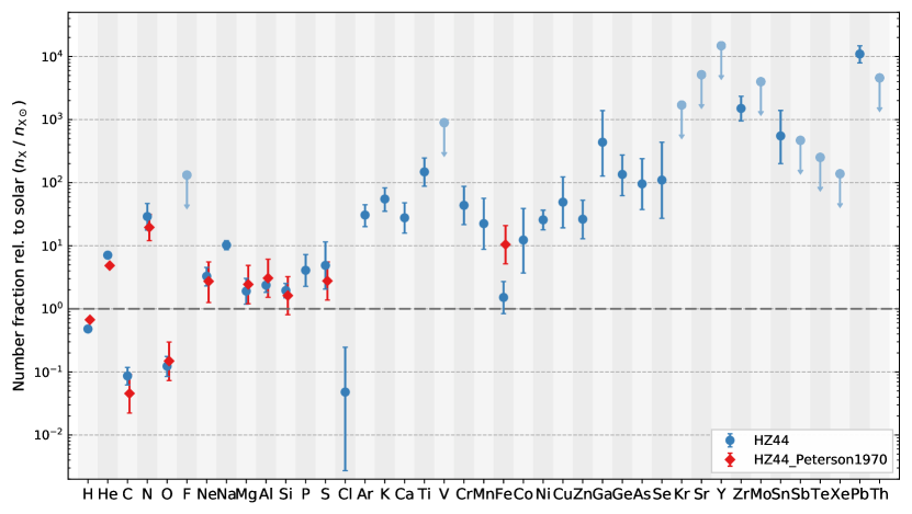
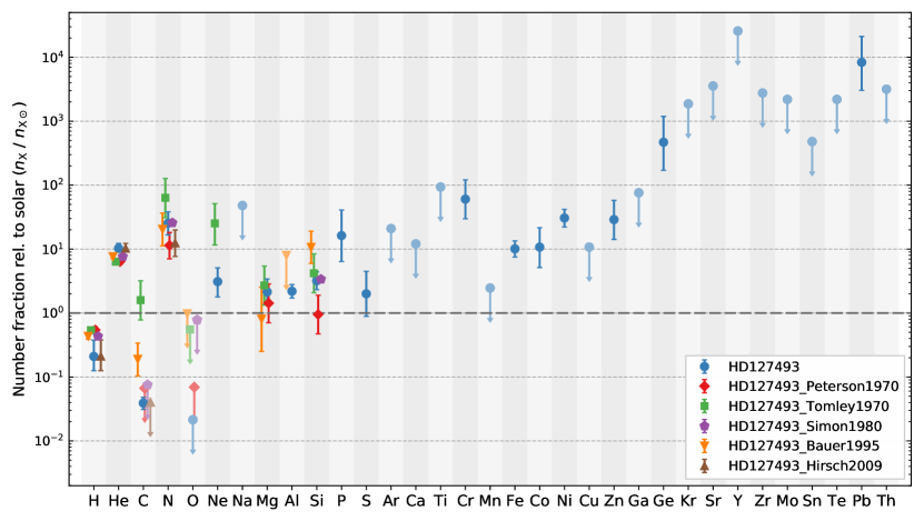
Figure 14: Same as Fig. 13 but for the comparison of abundances derived in this paper with literature values.

A.3 Abundances and stellar spectra

Table 11: Abundances of HZ 44 and HD 127493 as derived from visual/UVA and FUV data.

	Abundance ($\log n_{\mathrm{X}}/n_{\mathrm{H}}$)		Mass fraction ($\beta_{\mathrm{X}}$)		Number fraction ($\log n_{\mathrm{X}}$)		Abundance ($\log n_{\mathrm{X}}/n_{\mathrm{X,\odot}}$)
Element	HZ 44	HD 127493	HZ 44	HD 127493	HZ 44	HD 127493	HZ 44	HD 127493
H	0.00${}^{+0.00}_{-0.00}$	0.00${}^{+0.00}_{-0.00}$	-0.79${}^{+0.03}_{-0.03}$	-1.26${}^{+0.25}_{-0.21}$	-0.36${}^{+0.03}_{-0.03}$	-0.71${}^{+0.26}_{-0.22}$	-0.32${}^{+0.03}_{-0.03}$	-0.68${}^{+0.26}_{-0.22}$
He	0.10${}^{+0.05}_{-0.05}$	0.62${}^{+0.30}_{-0.30}$	-0.09${}^{+0.01}_{-0.01}$	-0.03${}^{+0.02}_{-0.01}$	-0.26${}^{+0.02}_{-0.02}$	-0.09${}^{+0.08}_{-0.04}$	0.85${}^{+0.02}_{-0.02}$	1.01${}^{+0.08}_{-0.05}$
C	-4.31${}^{+0.13}_{-0.13}$	-4.30${}^{+0.08}_{-0.08}$	-4.02${}^{+0.13}_{-0.13}$	-4.48${}^{+0.11}_{-0.09}$	-4.67${}^{+0.13}_{-0.13}$	-5.01${}^{+0.08}_{-0.08}$	-1.06${}^{+0.14}_{-0.14}$	-1.41${}^{+0.09}_{-0.10}$
N	-2.39${}^{+0.20}_{-0.20}$	-2.08${}^{+0.17}_{-0.17}$	-2.03${}^{+0.20}_{-0.20}$	-2.19${}^{+0.18}_{-0.18}$	-2.74${}^{+0.20}_{-0.20}$	-2.80${}^{+0.17}_{-0.17}$	1.46${}^{+0.21}_{-0.21}$	1.41${}^{+0.18}_{-0.18}$
O	-3.90${}^{+0.15}_{-0.15}$	¡-4.30+0.20	-3.49${}^{+0.15}_{-0.15}$	¡-4.35+0.21	-4.26${}^{+0.15}_{-0.15}$	¡-5.01+0.20	-0.91${}^{+0.16}_{-0.16}$	¡-1.67+0.20
F	¡-5.00+0.40		¡-4.51+0.40		¡-5.36+0.40		¡2.12+0.45
Ne	-3.23${}^{+0.11}_{-0.11}$	-2.90${}^{+0.20}_{-0.20}$	-2.72${}^{+0.11}_{-0.11}$	-2.85${}^{+0.21}_{-0.21}$	-3.59${}^{+0.11}_{-0.11}$	-3.61${}^{+0.20}_{-0.20}$	0.52${}^{+0.14}_{-0.15}$	0.49${}^{+0.21}_{-0.24}$
Na	-4.43${}^{+0.06}_{-0.06}$	¡-3.40+0.30	-3.86${}^{+0.06}_{-0.06}$	¡-3.29+0.30	-4.79${}^{+0.06}_{-0.06}$	¡-4.11+0.30	1.01${}^{+0.07}_{-0.07}$	¡1.68+0.30
Mg	-3.80${}^{+0.20}_{-0.20}$	-3.39${}^{+0.20}_{-0.20}$	-3.20${}^{+0.20}_{-0.20}$	-3.26${}^{+0.21}_{-0.21}$	-4.16${}^{+0.20}_{-0.20}$	-4.10${}^{+0.20}_{-0.20}$	0.28${}^{+0.20}_{-0.21}$	0.33${}^{+0.20}_{-0.21}$
Al	-4.86${}^{+0.11}_{-0.11}$	-4.53${}^{+0.10}_{-0.10}$	-4.21${}^{+0.11}_{-0.11}$	-4.35${}^{+0.12}_{-0.11}$	-5.21${}^{+0.11}_{-0.11}$	-5.24${}^{+0.10}_{-0.10}$	0.38${}^{+0.11}_{-0.11}$	0.34${}^{+0.10}_{-0.11}$
Si	-3.88${}^{+0.11}_{-0.11}$	-3.31${}^{+0.14}_{-0.14}$	-3.22${}^{+0.11}_{-0.11}$	-3.11${}^{+0.15}_{-0.14}$	-4.24${}^{+0.11}_{-0.11}$	-4.02${}^{+0.14}_{-0.13}$	0.29${}^{+0.11}_{-0.12}$	0.51${}^{+0.14}_{-0.14}$
P	-5.66${}^{+0.25}_{-0.25}$	-4.70${}^{+0.40}_{-0.40}$	-4.96${}^{+0.25}_{-0.25}$	-4.46${}^{+0.40}_{-0.41}$	-6.02${}^{+0.25}_{-0.25}$	-5.41${}^{+0.40}_{-0.40}$	0.61${}^{+0.25}_{-0.25}$	1.21${}^{+0.40}_{-0.40}$
S	-3.87${}^{+0.37}_{-0.37}$	-3.90${}^{+0.35}_{-0.35}$	-3.16${}^{+0.37}_{-0.37}$	-3.65${}^{+0.35}_{-0.36}$	-4.23${}^{+0.37}_{-0.37}$	-4.61${}^{+0.35}_{-0.35}$	0.69${}^{+0.37}_{-0.38}$	0.30${}^{+0.35}_{-0.35}$
Cl	-7.50${}^{+0.70}_{-0.70}$		-6.74${}^{+0.70}_{-0.70}$		-7.86${}^{+0.70}_{-0.70}$		-1.32${}^{+0.71}_{-1.25}$
Ar	-3.79${}^{+0.11}_{-0.11}$	¡-3.60+0.20	-2.98${}^{+0.11}_{-0.11}$	¡-3.25+0.21	-4.15${}^{+0.11}_{-0.11}$	¡-4.31+0.20	1.49${}^{+0.16}_{-0.18}$	¡1.32+0.23
K	-4.91${}^{+0.16}_{-0.16}$		-4.11${}^{+0.16}_{-0.16}$		-5.27${}^{+0.16}_{-0.16}$		1.74${}^{+0.18}_{-0.19}$
Ca	-3.90${}^{+0.24}_{-0.24}$	¡-3.90+0.20	-3.08${}^{+0.24}_{-0.24}$	¡-3.55+0.21	-4.25${}^{+0.24}_{-0.24}$	¡-4.61+0.20	1.44${}^{+0.24}_{-0.24}$	¡1.08+0.20
Ti	-4.56${}^{+0.22}_{-0.22}$	¡-4.40+0.25	-3.67${}^{+0.22}_{-0.22}$	¡-3.98+0.26	-4.92${}^{+0.22}_{-0.22}$	¡-5.11+0.25	2.17${}^{+0.22}_{-0.23}$	¡1.97+0.25
V	¡-4.80+0.40		¡-3.88+0.40		¡-5.16+0.40		¡2.95+0.40
Cr	-4.40${}^{+0.30}_{-0.30}$	-3.90${}^{+0.30}_{-0.30}$	-3.47${}^{+0.30}_{-0.30}$	-3.44${}^{+0.30}_{-0.31}$	-4.76${}^{+0.30}_{-0.30}$	-4.61${}^{+0.30}_{-0.30}$	1.64${}^{+0.30}_{-0.31}$	1.78${}^{+0.30}_{-0.31}$
Mn	-4.90${}^{+0.40}_{-0.40}$	¡-5.50+0.30	-3.95${}^{+0.40}_{-0.40}$	¡-5.02+0.30	-5.26${}^{+0.40}_{-0.40}$	¡-6.21+0.30	1.35${}^{+0.40}_{-0.41}$	¡0.39+0.30
Fe	-4.00${}^{+0.25}_{-0.25}$	-2.82${}^{+0.12}_{-0.12}$	-3.04${}^{+0.25}_{-0.25}$	-2.33${}^{+0.14}_{-0.13}$	-4.36${}^{+0.25}_{-0.25}$	-3.53${}^{+0.12}_{-0.12}$	0.18${}^{+0.25}_{-0.26}$	1.00${}^{+0.12}_{-0.13}$
Co	-5.60${}^{+0.50}_{-0.50}$	-5.30${}^{+0.30}_{-0.30}$	-4.62${}^{+0.50}_{-0.50}$	-4.78${}^{+0.30}_{-0.31}$	-5.96${}^{+0.50}_{-0.50}$	-6.01${}^{+0.30}_{-0.30}$	1.09${}^{+0.50}_{-0.52}$	1.03${}^{+0.30}_{-0.32}$
Ni	-4.05${}^{+0.15}_{-0.15}$	-3.61${}^{+0.13}_{-0.13}$	-3.07${}^{+0.15}_{-0.15}$	-3.10${}^{+0.15}_{-0.14}$	-4.41${}^{+0.15}_{-0.15}$	-4.33${}^{+0.13}_{-0.13}$	1.41${}^{+0.15}_{-0.16}$	1.49${}^{+0.14}_{-0.14}$
Cu	-5.80${}^{+0.40}_{-0.40}$	¡-6.10+0.40	-4.79${}^{+0.40}_{-0.40}$	¡-5.55+0.40	-6.16${}^{+0.40}_{-0.40}$	¡-6.81+0.40	1.69${}^{+0.40}_{-0.41}$	¡1.03+0.40
Zn	-5.70${}^{+0.30}_{-0.30}$	-5.30${}^{+0.30}_{-0.30}$	-4.67${}^{+0.30}_{-0.30}$	-4.74${}^{+0.30}_{-0.31}$	-6.06${}^{+0.30}_{-0.30}$	-6.01${}^{+0.30}_{-0.30}$	1.42${}^{+0.30}_{-0.31}$	1.46${}^{+0.30}_{-0.31}$
Ga	-6.00${}^{+0.50}_{-0.50}$	¡-6.40+0.40	-4.95${}^{+0.50}_{-0.50}$	¡-5.81+0.40	-6.36${}^{+0.50}_{-0.50}$	¡-7.11+0.40	2.64${}^{+0.50}_{-0.54}$	¡1.88+0.40
Ge	-5.90${}^{+0.30}_{-0.30}$	-5.00${}^{+0.40}_{-0.40}$	-4.83${}^{+0.30}_{-0.30}$	-4.39${}^{+0.40}_{-0.41}$	-6.26${}^{+0.30}_{-0.30}$	-5.71${}^{+0.40}_{-0.40}$	2.13${}^{+0.31}_{-0.34}$	2.67${}^{+0.40}_{-0.44}$
As	-7.40${}^{+0.40}_{-0.40}$		-6.31${}^{+0.40}_{-0.40}$		-7.76${}^{+0.40}_{-0.40}$		1.98${}^{+0.40}_{-0.41}$
Se	-6.30${}^{+0.60}_{-0.60}$		-5.19${}^{+0.60}_{-0.60}$		-6.66${}^{+0.60}_{-0.60}$		2.04${}^{+0.60}_{-0.61}$
Kr	¡-5.20+0.60	¡-4.80+0.40	¡-4.07+0.60	¡-4.13+0.40	¡-5.56+0.60	¡-5.51+0.40	¡3.23+0.60	¡3.27+0.40
Sr	¡-5.10+0.60	¡-4.90+0.30	¡-3.95+0.60	¡-4.21+0.30	¡-5.46+0.60	¡-5.61+0.30	¡3.71+0.60	¡3.55+0.30
Y	¡-5.30+0.20	¡-4.70+0.30	¡-4.14+0.20	¡-4.01+0.30	¡-5.66+0.20	¡-5.41+0.30	¡4.17+0.20	¡4.41+0.30
Zr	-5.92${}^{+0.19}_{-0.19}$	¡-5.30+0.20	-4.75${}^{+0.19}_{-0.19}$	¡-4.60+0.21	-6.28${}^{+0.19}_{-0.19}$	¡-6.01+0.20	3.18${}^{+0.19}_{-0.20}$	¡3.44+0.20
Mo	¡-6.20+0.40	¡-6.10+0.40	¡-5.01+0.40	¡-5.37+0.40	¡-6.56+0.40	¡-6.81+0.40	¡3.60+0.40	¡3.34+0.40
Sn	-6.90${}^{+0.40}_{-0.40}$	¡-6.60+0.40	-5.61${}^{+0.40}_{-0.40}$	¡-5.78+0.40	-7.26${}^{+0.40}_{-0.40}$	¡-7.31+0.40	2.74${}^{+0.40}_{-0.44}$	¡2.68+0.40
Sb	¡-8.00+0.50		¡-6.70+0.50		¡-8.36+0.50		¡2.67+0.50
Te	¡-7.10+0.40	¡-5.80+0.40	¡-5.78+0.40	¡-4.95+0.40	¡-7.46+0.40	¡-6.51+0.40	¡2.40+0.40	¡3.34+0.40
Xe	¡-7.30+0.40		¡-5.97+0.40		¡-7.66+0.40		¡2.14+0.40
Pb	-5.89${}^{+0.09}_{-0.09}$	-5.65${}^{+0.40}_{-0.40}$	-4.36${}^{+0.09}_{-0.09}$	-4.59${}^{+0.40}_{-0.41}$	-6.25${}^{+0.09}_{-0.09}$	-6.36${}^{+0.40}_{-0.40}$	4.04${}^{+0.13}_{-0.14}$	3.92${}^{+0.40}_{-0.44}$
Th	¡-8.00+0.30	¡-7.80+0.30	¡-6.42+0.30	¡-6.69+0.30	¡-8.36+0.30	¡-8.51+0.30	¡3.66+0.31	¡3.50+0.31

This section presents our final abundance values (Table 11) as well as a comparison between the full observed and final synthetic spectra of HZ 44 and HD 127493 (Fig. 15 to Fig. 31). In the synthetic spectra, elements with upper limits only are included at their upper limit. The synthetic spectra are convolved with a Gaussian kernel (constant for GHRS, but wavelength-depended for all echelle spectrographs) to match the resolution of the respective spectrograph. The strongest photospheric metal lines are labeled with magenta marks, interstellar lines are labeled with green marks. At the bottom of each spectral range we also show the residual between the observation and our final model. A proper normalization of the HIRES spectrum of HZ 44 was only possible using the final synthetic spectrum as a template. Thus the shape of broad hydrogen and helium lines in the HIRES spectra is adjusted during the normalization procedure to fit the shape of the synthetic spectrum. However, the shape of the sharp metal lines, that are of interest in the HIRES spectra, are not affected by the normalization procedure. The optical spectra of HZ 44 and HD 127493 are shown up to 6710 Å since the number of metal lines at longer wavelengths is very limited.

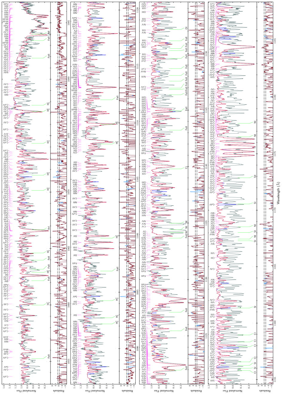
Figure 15: FUSE spectrum of HZ 44 (gray) and the final model (red, with heavy metals: blue).

Figure 16: FUSE spectrum of HZ 44 (gray) and the final model (red, with heavy metals: blue).

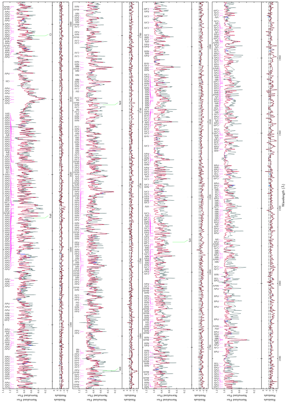
Figure 17: IUE spectrum of HZ 44 (gray) and the final model (red, with heavy metals: blue).

Figure 18: IUE spectrum of HZ 44 (gray) and the final model (red, with heavy metals: blue).

Figure 19: HIRES spectrum of HZ 44 (gray) and the final model (red).

Figure 20: HIRES spectrum of HZ 44 (gray) and the final model (red).

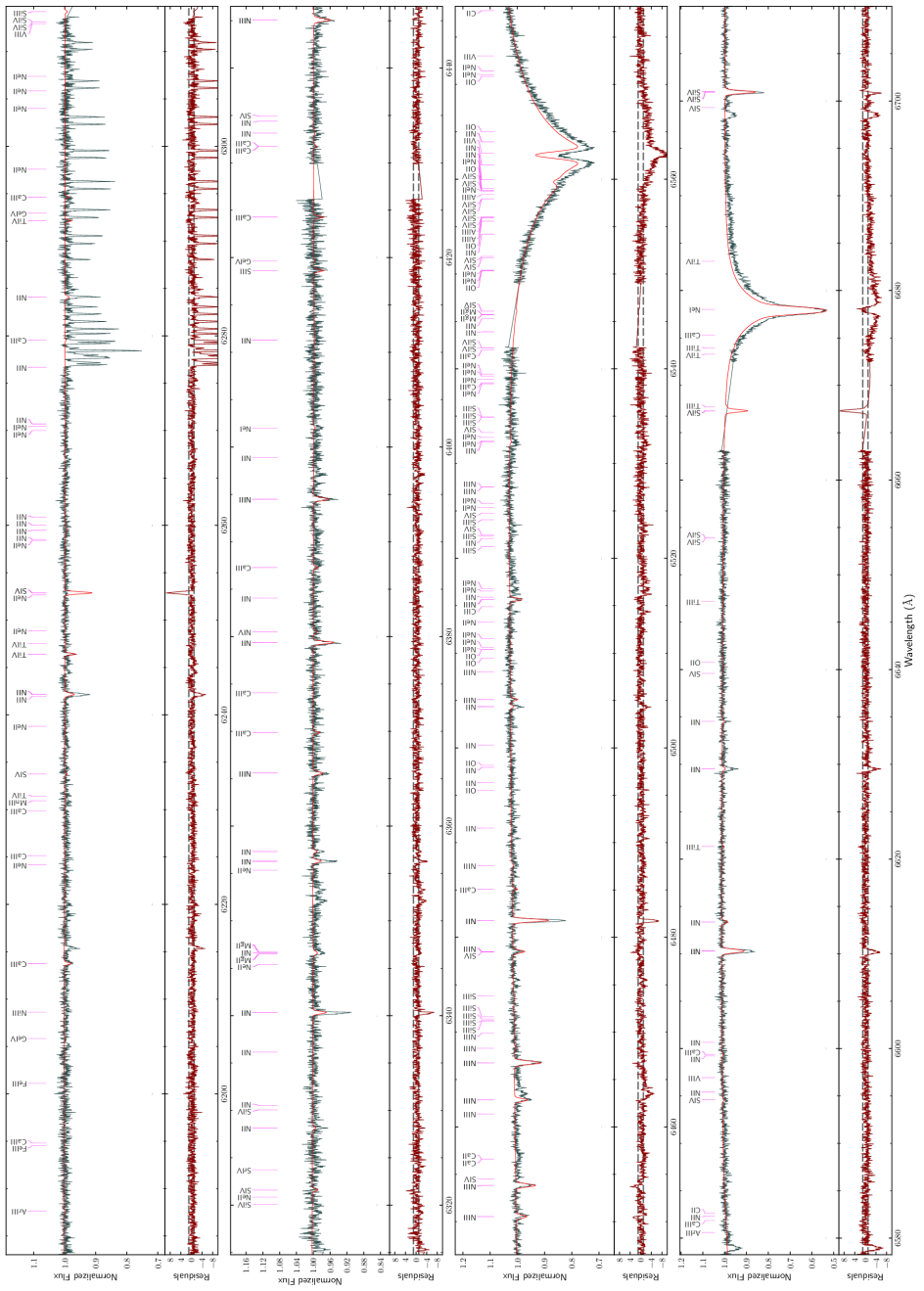
Figure 21: HIRES spectrum of HZ 44 (gray) and the final model (red).

Figure 22: HIRES spectrum of HZ 44 (gray) and the final model (red).

Figure 23: HIRES spectrum of HZ 44 (gray) and the final model (red).

Figure 24: HIRES spectrum of HZ 44 (gray) and the final model (red).

Figure 25: HIRES spectrum of HZ 44 (gray) and the final model (red).

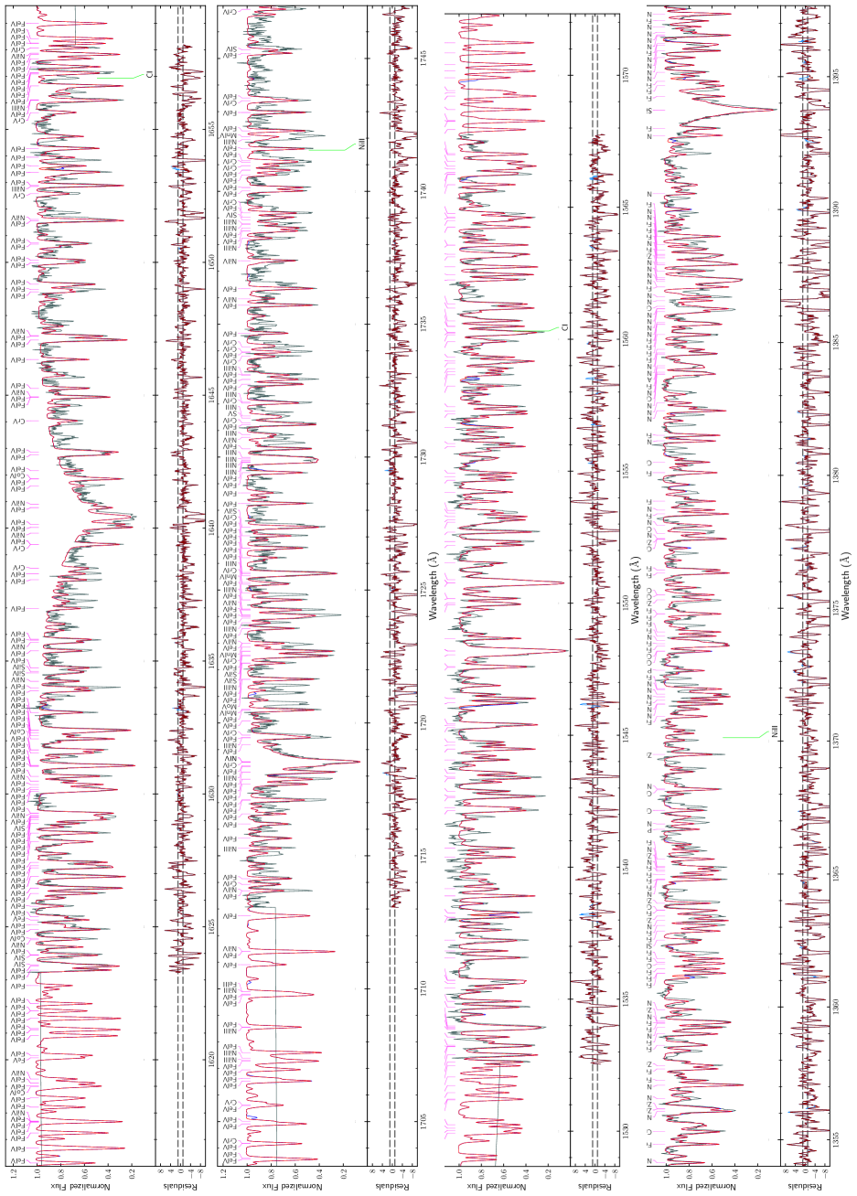
Figure 26: GHRS spectrum of HD 127493 (gray) and the final model (red, with heavy metals: blue).

Figure 27: GHRS spectrum of HD 127493 (gray) and the final model (red, with heavy metals: blue).

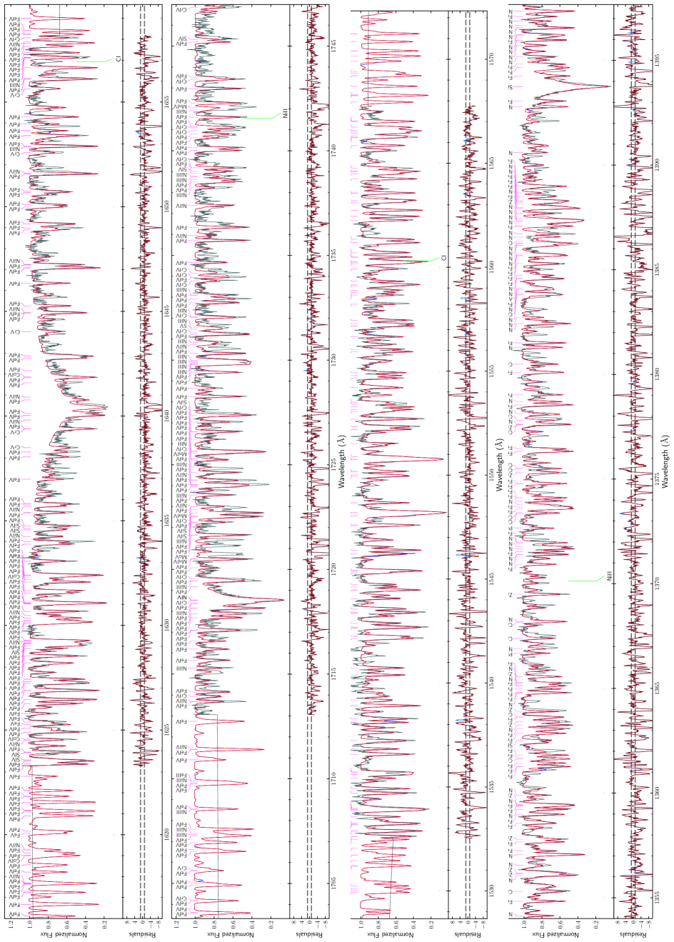
Figure 28: GHRS spectrum of HD 127493 (gray) and the final model (red, with heavy metals: blue).

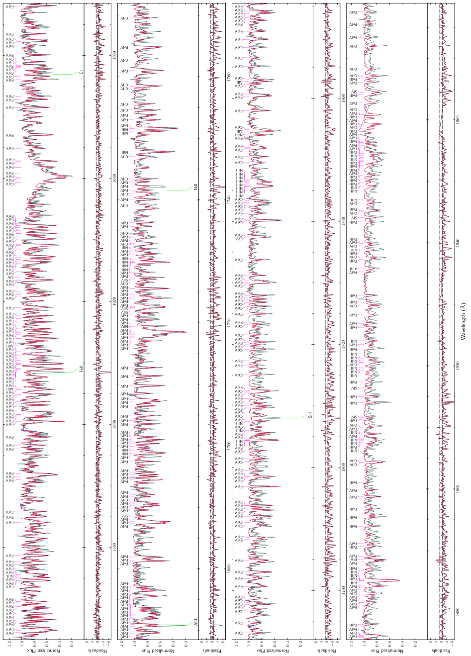
Figure 29: IUE spectrum of HD 127493 (gray) and the final model (red, with heavy metals: blue).

Figure 30: IUE spectrum of HD 127493 (gray) and the final model (red, with heavy metals: blue).

Figure 31: FEROS spectrum of HD 127493 (gray) and the final model (red).

Figure 32: FEROS spectrum of HD 127493 (gray) and the final model (red).

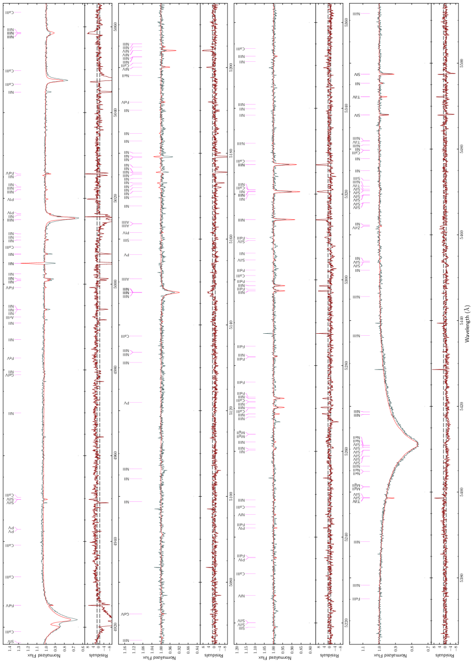
Figure 33: FEROS spectrum of HD 127493 (gray) and the final model (red).

Figure 34: FEROS spectrum of HD 127493 (gray) and the final model (red).

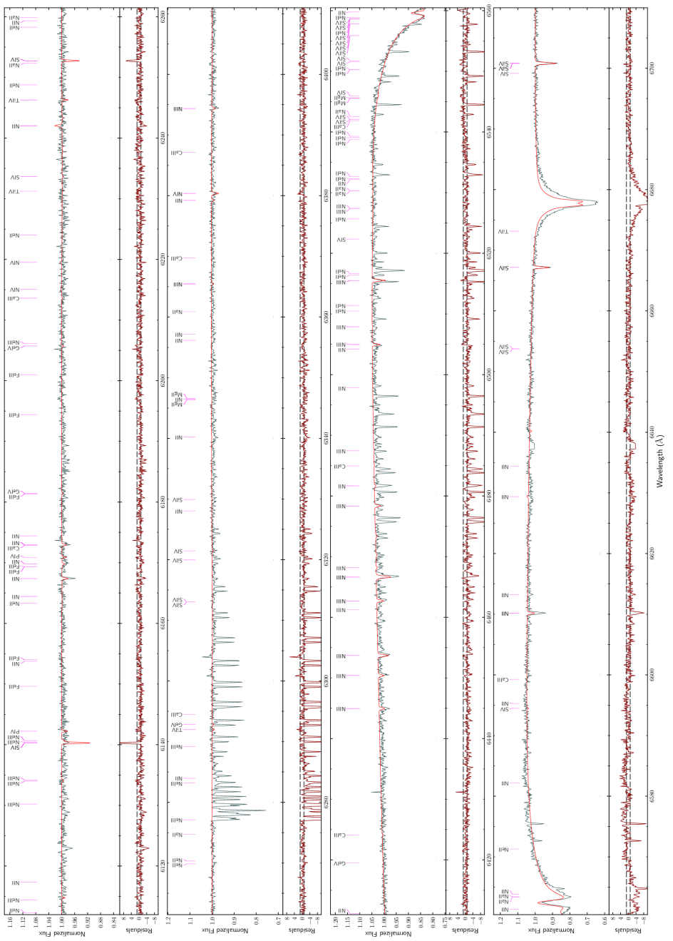
Figure 35: FEROS spectrum of HD 127493 (gray) and the final model (red).