Trace formulas for general Hermitian matrices: Unitary scattering approach and periodic orbits on an associated graph

Abstract

Two trace formulas for the spectra of arbitrary Hermitian matrices are derived by transforming the given Hermitian matrix $H$ to a unitary analogue. In the first type the unitary matrix is $e^{i(\lambda{\mathbb{I}}-H)}$ where $\lambda$ is the spectral parameter. The new feature is that the spectral parameter appears in the final form as an argument of Eulerian polynomials – thus connecting the periodic orbits to combinatorial objects in a novel way. To obtain the second type, one expresses the input in terms of a unitary scattering matrix in a larger Hilbert space. One of the surprising features here is that the locations and radii of the spectral discs of Gershgorin’s theorem appear naturally as the pole parameters of the scattering matrix. Both formulas are discussed and possible applications are outlined.

I Introduction

Trace formula is a generic name for relations which connect between spectral information and geometric or dynamical information pertaining to the same operator and its domain. Since it was first introduced by A. Selberg Selberg , it has been one of the main tools in many fields of research, ranging between number theory, spectral geometry, graphs (combinatorial and quantum) and the semi-classical theory of integrable and chaotic area preserving dynamical systems Gutzwiller1970 ; Gutzwiller1971 ; Gutzwillerbook ; Balianbloch ; Berrytabor ; Ozorio ; qsoc . Typically, the spectral information is expressed in terms of the spectral density or the spectral counting function. The geometrical information resides in the properties of periodic structures or orbits, such as closed walks on connected vertices in a graph, periodic classical trajectories, periodic geodesics on closed surfaces, etc.

A simple example arises in the study of the spectra finite of Hermitian matrices. The spectral density of a $N\times N$ Hermitian matrix $H$ with spectrum denoted by $\{\lambda_{j}\}_{j=1}^{N}$ can be expressed in terms of the resolvent (Green function) $G(z)=(z{\mathbb{I}}-H)^{-1}$

$$\rho(\lambda)=\sum_{j=1}^{N}\delta({\lambda}-\lambda_{j})=\frac{1}{\pi}\lim_{\epsilon\rightarrow 0}\mathrm{Im}\,\left[\mathrm{tr}\,G(\lambda+i\epsilon)\right].$$ (1)

The Green function $G(z)$ is a meromorphic function on the complex plane $z\in\mathbb{C}$ with poles at the eigenvalues of $H$. While the expansion $\mathrm{tr}\,G(z)=\sum_{n=0}^{\infty}\frac{\mathrm{tr}\,H^{n}}{z^{n+1}}$ only converges absolutely for $z$ outside the spectral radius, one may substitute this expansion in (1) and take $\epsilon\to 0$ if one considers this as a distributional identity where the series converges subject to integration with respect to an appropriate set of test functions. In this sense one obtains

$$\rho(\lambda)=\frac{1}{\pi}\lim_{\epsilon\rightarrow 0}\mathrm{Im}\,\left[\sum_{n=0}^{\infty}\frac{\mathrm{tr}\,H^{n}}{(\lambda+i\epsilon)^{n+1}}\right].$$ (2)

Thus, the spectral density is expressed in terms of the geometrical information embedded in $\mathrm{tr}\,H^{n}$. The connection to “geometry” comes by recalling that

$$\mathrm{tr}\,H^{n}=\sum_{\{1\leq i_{k}\leq N\}}H_{i_{1},i_{n}}H_{i_{n},i_{n-1}}\cdots H_{i_{2},i_{1}}$$ (3)

which can be viewed as a sum over weighted periodic walks on a connected graph on $N$ vertices (with self loops but no multiple edges), where the weight on the edge ${i,j}$ is the matrix element $H_{i,j}$. When $H$ is e.g., an adjacency matrix of a combinatorial graph, with $H_{i,j}\in[0,1])$, $\mathrm{tr}\,H^{n}$ counts the number of periodic walks with period $n$ on the graphs. This connection was used by E. Wigner wigner in deriving the semi-circle law by counting the mean number of periodic walks on random graphs.

The above example also illustrates an important characteristic of trace formulas: when they are written as equalities, they are formal, and cannot be used as numerical ones. Rather, they express relations whose contents can be elucidated by analytical continuation, or by application to appropriate test functions.

In the present work we derive and study two types of trace formulas, which, to the best of our knowledge were not previously formulated. Both of them express the spectral density or the spectral counting function of a Hermitian matrix $H$ in terms of (weighted) periodic orbits on an underlying graph in the sense explained above. The common feature of both approaches is that the spectral data of the original matrix $H$ is stored in a unitary matrix $S(\lambda)$ such that $\lambda=\lambda_{j}$ is an eigenvalue of $H$ if and only if the unitary matrix $S(\lambda)$ has a stationary eigenvector (that is an eigenvector $\mathbf{x}$ that satisfies $S(\lambda)\mathbf{x}=\mathbf{x}$). The two kinds of trace formulas that we present are derived from different choices of the matrix $S(\lambda)$.

In Sec. II we present the first approach where $S(\lambda)$ has the same dimension $N$ as $H$ and is constructed from the “evolution operator” $e^{-iHt}$ for a unit of time $t$ (without loss of generality we will set $t=1$). In this case the trace formula will be expressed in two different forms that involve the traces $\mathrm{tr}\,H^{n}$ and thus the same periodic orbits and weights on an underlying graph as described in (3). In the final expression, the Polylogarithmic functions of negative index (which may be expressed in terms of Eulerian polynomials) play a crucial role.

In Sec. III we present a rather different approach. There, we construct a unitary matrix $S(\lambda)$ that may be viewed as an evolution operator of a discrete time quantum walk on the directed edges of the underlying simple graph without the self-loops present in the first approach. The dimension of the $S$ matrix is larger than $N$ and equals the number of non vanishing off-diagonal matrix elements (if $H_{vw}=H_{wv}^{*}\neq 0$ and $w\neq v$ both matrix elements are counted). It enables writing a trace formula in yet another form, albeit the input to the effective weights and the phases carried by the paths, are different than the ones used to compute $\mathrm{tr}\,H^{n}$ in the first approach. This second approach is a generalization of previous work uzy where a similar trace formula has been derived for discrete graph Laplacians. In spectral graph theory there is a long history of expressing the spectra of (weighted) graph Laplacians in terms of walks or periodic orbits on the directed edges. Starting from the Ihara $\zeta$-function ihara1 ; ihara2 these use a number of determinantal equalities that have been developed by various authors traceformula_regI ; traceformula_regII ; hashimoto1 ; hashimoto_hori ; hashimoto2 ; hashimoto3 ; bass ; bartholdi ; kotani-sunada ; nalini . Our approach leads to a determinantal equality that is, to the best of our knowledge new and belongs in the same context. A main difference between our approach and the ones found in the literature is its generality as one may start from an arbitrary complex Hermitian matrix while the most general equalities available in the literature are for graph Laplacians nalini (a subset of real symmetric matrices). In the Ihara trace formula and many of its generalizations the sum over periodic orbits is reduced to non-backscattering orbits. This simplification does not apply to our approach however.

In Sec. IV we conclude this paper with a general outlook.

Note: in order to make a clear distinction between quantities related to the two trace formulas, we shall distinguish them by a suffix $I$ or $II$.

II Approach I: a trace formula based on the time evolution operator

Let $H$ be a Hermitian matrix of dimension $N$, with spectrum $\{\lambda_{i}\}_{i=1}^{N}$ consisting of the roots of the characteristic polynomial

$$\zeta_{H}(\lambda)=\mathrm{det}\,(\lambda{\mathbb{I}}-H).$$ (4)

We write the Heaviside step function as $\theta(x)$ and denote by

$$\mathcal{N}(\lambda)=\sum_{j=1}^{N}\theta(\lambda-\lambda_{j})$$ (5)

the number of eigenvalues (zeros of the characteristic polynomial with multiplicities) which are smaller or equal $\lambda$. We will refer to $\mathcal{N}({\lambda})$ as the (spectral) counting function and its (formal) derivative

$$\rho(\lambda)=\sum_{j=1}^{N}\delta(\lambda-\lambda_{j})$$ (6)

as the density of states.

In this section we shall present two variants of a trace formula which express $\mathcal{N}(\lambda)$ in terms of the traces of powers of $H$ in a different way than given by (2) in the introduction Sec I. For this we consider the unitary $N\times N$ matrix

$$S_{I}(\lambda)=e^{i(\lambda{\mathbb{I}}-H)}$$ (7)

such that $S_{I}(0)=e^{-iH}$ is equal to the time evolution operator $e^{-iHt}$ for a unit of time $t$ where the units have been chosen such that $t=1$. Without loss of generality we assume that the spectrum is normalized and shifted such that it is in the real interval $(-\pi,\pi)$, and ordered monotonically $\lambda_{i}\leq\lambda_{i+1}$. This ensures that there is a one-to-one and order-preserving correspondence between the eigenvalues $\{e^{-i\lambda_{j}}\}$ of $S_{I}(0)$ on the unit circle and the eigenvalues $\{\lambda_{j}\}$ of $H$. Moreover, strict positivity of the gap

$$\delta:=\pi-\mathrm{max}(|\lambda_{i}|)=\mathrm{min}(\pi-\lambda_{N},\lambda_{1}+\pi)>0$$ (8)

will be assumed in order to ensure convergence of the trace formulas. This restriction can always be met by a trivial rescaling $H\mapsto cH$ with some $c\in{\mathbb{R}}$. We also introduce the secular function

$$\zeta_{I}(\lambda)=\mathrm{det}\,\left({\mathbb{I}}-S_{I}(\lambda)\right)$$ (9)

which is a periodic function $\zeta_{I}(\lambda+2\pi)=\zeta_{I}(\lambda)$ with $N$ zeros in the interval $\lambda\in(-\pi,\pi)$ at the eigenvalues $\lambda=\lambda_{j}$ of $H$.

II.1 The first variant of the trace formula based on $S_{I}(\lambda)$

Restricting $\lambda\in(-\pi,\pi)$ the first variant of the trace formula is given by

$$\mathcal{N}_{I}(\lambda)= \overline{\mathcal{N}}_{I}(\lambda)+\mathcal{N}_{I}^{(\mathrm{osc})}(\lambda)$$ (10a)

$$\overline{\mathcal{N}}_{I}(\lambda)= \frac{N\lambda-\mathrm{tr}\,H}{2\pi}+\frac{N}{2}$$ (10b)

$$\mathcal{N}_{I}^{(\mathrm{osc})}(\lambda)= \frac{1}{\pi}\lim_{\epsilon\rightarrow 0^{+}}\mathrm{Im}\,\left\{\sum_{n=1}^{\infty}\sum_{s=0}^{\infty}e^{-i\frac{\pi}{2}s}\ \frac{\mathrm{tr}\,H^{s}}{s!}\ n^{s-1}\ e^{(i\lambda-\epsilon)n}\right\}$$

$$= \frac{1}{\pi}\lim_{\epsilon\rightarrow 0^{+}}\mathrm{Im}\,\left\{\sum_{s=0}^{\infty}e^{-i\frac{\pi}{2}s}\ \frac{\mathrm{tr}\,H^{s}}{s!}\sum_{n=1}^{\infty}n^{s-1}\ e^{(i\lambda-\epsilon)n}\right\}\ .$$ (10c)

The corresponding expression for the density of states reads

$$\rho_{I}(\lambda)= \overline{\rho}_{I}(\lambda)+\rho_{I}^{(\mathrm{osc})}$$ (11a)

$$\overline{\rho}_{I}(\lambda)= \frac{N}{2\pi}$$ (11b)

$$\rho_{I}^{(\mathrm{osc})}= \frac{1}{\pi}\lim_{\epsilon\rightarrow 0^{+}}\mathrm{Re}\,\left\{\sum_{s=0}^{\infty}\ e^{-i\frac{\pi}{2}s}\ \frac{\mathrm{tr}\,H^{s}}{s!}\sum_{n=1}^{\infty}n^{s}\ e^{(i\lambda-\epsilon)n}\right\}\ .$$ (11c)

We will refer to $\overline{\mathcal{N}}_{I}({\lambda})$ and $\overline{\rho}_{I}(\lambda)$ as the smooth part and to $\mathcal{N}_{I}^{(\mathrm{osc})}(\lambda)$ and $\rho_{I}^{(\mathrm{osc})}$ as the oscillating parts. One should note that we have defined $\mathcal{N}_{I}(\lambda)$ and $\rho_{I}(\lambda)$ only for $|\lambda|<\pi$ while $\mathcal{N}(\lambda)$ and $\rho(\lambda)$ are defined on the real line. If one uses the given expressions for the trace formulas one finds that the spectrum is repeated periodically such that $\rho_{I}(\lambda+2\pi)=\rho_{I}(\lambda)$, $\overline{\mathcal{N}}_{I}(\lambda+2\pi)=N+\overline{\mathcal{N}}_{I}(\lambda)$ and $\mathcal{N}_{I}^{(\mathrm{osc})}(\lambda+2\pi)=\mathcal{N}_{I}^{(\mathrm{osc})}(\lambda)$ so outside the interval $|\lambda|<\pi$ one generally has $\mathcal{N}_{I}(\lambda)\neq\mathcal{N}(\lambda)$ and $\rho_{I}(\lambda)\neq\rho(\lambda)$. This periodic behaviour makes this approach fundamentally different from the second approach that we will lay out in Sec. III where no such periodicity will appear.

The trace formula (10) can be derived from the secular equation $\zeta_{I}(\lambda)=0$. Using Cauchy’s theorem, the identity $\log\mathrm{det}\,({\mathbb{I}}-S)=\mathrm{tr}\,\log({\mathbb{I}}-S)$ and expanding $e^{-iH}$ in a Taylor series gives (10). Note that while the double sum in the limit converges for any $\epsilon>0$ it does not converge absolutely for arbitrarily small $\epsilon>0$ as

$$\sum_{n=1}^{\infty}\sum_{s=0}^{\infty}\left|e^{-i\frac{\pi}{2}s}\ \frac{\mathrm{tr}\,H^{s}}{s!}\ n^{s-1}\ e^{(i\lambda-\epsilon)n}\right|=\sum_{n=1}^{\infty}\sum_{j=1}^{N}\frac{e^{n\left(|\lambda_{j}|-\epsilon\right)}}{n}$$ (12)

which converges only if $\epsilon>\mathrm{max}_{j=1}^{N}(|\lambda_{j}|)$ (thus, for any given matrix $H$ with a spectrum that satisfies the assumed restrictions one may choose $\epsilon=\pi$ to ensure convergence.) Nonetheless we formally interchange the two summations in the last line of (10) in order to arrive at an expression where $\mathrm{tr}\ H^{s}$ (and thus the periodic orbits) can be attributed a specific weight. Note that almost all interesting trace formulas express distributional identities. This applies to the present case as well and the interchange of summation just implies a suitable restriction to test functions that render the double summation absolutely convergent. In this case this is achieved by considering test functions $f(\lambda)$ defined for $\lambda\in(-\pi,\pi)$ by a Fourier series $f(\lambda)=\sum_{n=-\infty}^{\infty}f_{n}e^{i\lambda n}$ with $\lim\mathrm{sup}\ e^{\pi n}|f_{n}|<C$ for some constant $C$. This condition implies that the test functions are analytic on the real axis. Trace formulas are often used as formal devices far beyond the rigorous applicability. Indeed we will show later (in Sec. II.4) that this trace formula gives correct results even when formally applied to test functions that do not obey the stated rigorous restrictions. For practical purposes one can achieve numerical convergence in the trace formula (10) for the spectral counting function by introducing appropriate $\epsilon$-dependent cut-offs for the double sum, see App. A.

An equivalent derivation starts with the expression

$$\theta(\lambda-\lambda_{j})= \frac{\lambda-\lambda_{j}}{2\pi}+\frac{1}{2}-\lim_{\epsilon\to 0}\mathrm{Im}\ \log\left(1-e^{i(\lambda-\lambda_{j})-\epsilon}\right)$$

$$= \frac{\lambda-\lambda_{j}}{2\pi}+\frac{1}{2}+\lim_{\epsilon\to 0}\mathrm{Im}\sum_{n=1}^{\infty}\frac{e^{in(\lambda-\lambda_{j})-n\epsilon)}}{n}$$

$$= \frac{\lambda-\lambda_{j}}{2\pi}+\frac{1}{2}+\lim_{\epsilon\to 0}\mathrm{Im}\sum_{n=1}^{\infty}\sum_{s=0}^{\infty}e^{-i\frac{\pi}{2}s}\frac{\lambda_{j}^{s}}{s!}n^{s-1}e^{(i\lambda-\epsilon)n}$$ (13)

which is valid for $\lambda\in(-\pi,\pi)$. Summing this identity over the $N$ eigenvalues $\{\lambda_{j}\}$ then gives the trace formula (10).

II.2 The second variant of the trace formula based on $S_{I}(\lambda)$: Polylogarithms and Eulerian polynomials

The second variant of the trace formula is obtained by noting that the sum over $n$ in the trace formula (10) can be expressed in terms of the Polylogarithm functions

$$\mathrm{Li}_{-s}\left(z\right):=\sum_{n=1}^{\infty}n^{s}z^{n}.$$ (14)

Performing the sum over $n$ in (10) one then obtains the trace formula

$$\mathcal{N}_{I}(\lambda)= \overline{\mathcal{N}}_{I}(\lambda)+\mathcal{N}_{I}^{(\mathrm{osc})}(\lambda)$$ (15a)

$$\overline{\mathcal{N}}_{I}(\lambda)= \frac{N\lambda-\mathrm{tr}\,H}{2\pi}+\frac{N}{2}$$ (15b)

$$\mathcal{N}^{(\mathrm{osc})}_{I}(\lambda)= \frac{1}{\pi}\lim_{\epsilon\rightarrow 0^{+}}\mathrm{Im}\,\left\{\sum_{s=0}^{\infty}\ e^{-i\frac{\pi}{2}s}\ \frac{\mathrm{tr}\,H^{s}}{s!}\ \mathrm{Li}_{-s+1}\left(e^{(i\lambda-\epsilon)}\right)\right\}$$ (15c)

for the spectral counting function, and

$$\rho_{I}(\lambda)= \overline{\rho}_{I}(\lambda)+\rho^{(\mathrm{osc})}_{I}(\lambda)$$ (16a)

$$\overline{\rho}_{I}(\lambda)= \frac{N}{2\pi}$$ (16b)

$$\rho_{I}^{(\mathrm{osc})}(\lambda)= \frac{1}{\pi}\lim_{\epsilon\rightarrow 0^{+}}\mathrm{Re}\,\left\{\sum_{s=0}^{\infty}\ e^{-i\frac{\pi}{2}s}\ \frac{\mathrm{tr}\,H^{s}}{s!}\ \mathrm{Li}_{-s}\left(e^{(i\lambda-\epsilon)}\right)\right\}$$ (16c)

for the density of states. The relevant Polylogarithms are explicitly given by

$$\mathrm{Li}_{0}(z) =\frac{z}{1-z}$$ (17)

$$\mathrm{Li}_{1}(z) =-\log(1-z)$$ (18)

and the recursion

$$\mathrm{Li}_{-s}(z)=z\frac{\partial\mathrm{Li}_{1-s}(z)}{\partial z}=\left(z\frac{d}{dz}\right)^{s}\frac{z}{1-z}$$ (19)

for $s>0$. This implies that the Polylogarithms with negative index are rational functions

$$\mathrm{Li}_{-s}(z)=\frac{z}{(1-z)^{s+1}}A_{s}(z)$$ (20)

where $A_{s}(z)$ are known to be the Eulerian polynomials Eulerian (not to be confused with the Euler polynomials) which may be written as

$$A_{s}(z)=\sum_{k=0}^{s-1}A(s,k)z^{k}$$ (21)

in terms of the Eulerian numbers

$$A(s,k)=\sum_{m=0}^{k}(-1)^{m}\begin{pmatrix}s+1\\ m\end{pmatrix}(k+1-m)^{s}\ .$$ (22)

The Eulerian numbers are often denoted as $\genfrac{\langle}{\rangle}{0.0pt}{}{s}{k}=A(s,k)$ and they were introduced originally in a combinatorial context. Note that $A(s,s)=0$ which is the reason that the sum in (21) is often extended to include the term $k=s$. Note that (19) implies that near the pole, as $z\to 1$ one has $\mathrm{Li}_{-s}(z)\sim\frac{s!}{(1-z)^{s+1}}$ which shows that

$$A_{s}(1)=\sum_{k=0}^{s-1}A(s,k)=s!\ .$$ (23)

As the Eulerian numbers are real one also has $\mathrm{Li}_{-s}(z)^{*}=\mathrm{Li}_{-s}\left(z^{*}\right)$.

For the sake of completeness we mention yet another alternative expression for the trace formula which may be obtained by expressing $\mathrm{Li}_{-n}(z)$ in (15) and (16) as a polynomial in $\frac{z}{1-z}$

$$\mathrm{Li}_{-n}(z)=\sum_{k=0}^{n}k!S(n+1,k+1)\left(\frac{z}{1-z}\right)^{k+1}\ .$$ (24)

Here $S(n,k)$ are the Stirling numbers of the second kind

$$S(n,k)=\frac{1}{k!}\sum_{j=0}^{k}(-1)^{k-j}\begin{pmatrix}k\\ j\end{pmatrix}j^{n}$$ (25)

The Stirling numbers satisfy $S(n,n)=S(n,1)=1$. For fixed k and $n\gg 1,\ \ S(n,k)\sim\frac{k^{n}}{k!}$.

II.3 The trace formula as a sum over periodic orbits on an underlying graph

To the matrix $H$ we may associate the graph $\mathcal{G}_{I}$ with $N$ vertices. We enumerate the vertices and associate each to one dimension of the matrix $H$. The adjacency matrix $A_{I}$ of $\mathcal{G}_{I}$ is given by

$$A_{I,vw}=\begin{cases}1&\text{if $H_{vw}\neq 0$,}\\ 0&\text{if $H_{vw}=0$.}\end{cases}$$ (26)

So that there is an edge connecting two different vertices $v$ and $w\neq v$ if the corresponding off-diagonal element of $H_{vw}$ does not vanish, and a loop at vertex $v$ when the corresponding diagonal element $H_{vv}$ does not vanish. A periodic orbit $p=\overline{v_{1}v_{2}\dots v_{n_{p}}}$ on the graph $\mathcal{G}_{I}$ consists of a sequence of vertices $v_{k}$ ($k=1,\dots,n_{p}$) such that, for $k=1,\dots n_{p}$ the vertex $v_{k}$ is connected to $v_{k+1}$ by an edge (that is $A_{I,v_{k}v_{k+1}}=1$) and $v_{n_{p}}$ is also connected to $v_{1}$ ($A_{I,v_{n_{p}}v_{1}}=1$). Different starting points are considered equivalent ($\overline{v_{1}v_{2}\dots v_{n_{p}}}\equiv\overline{v_{2}\dots v_{n_{p}}v_{1}}$) and the integer $n_{p}$ is called the length of the periodic orbit. If $p=\overline{v_{1}v_{2}\dots v_{n_{p}}}$ we will always set $v_{0}\equiv v_{n_{p}}$ and $v_{n_{p}+1}=v_{1}$. A periodic orbit that is not a repetition of a shorter orbit is called primitive. Every periodic orbit is a repetition of a primitive orbit with repetition number $r_{p}$. To each periodic orbit $p$ of length $n_{p}$ we now associate the weight

$${\mathcal{W}_{I,p}}=\prod_{k=1}^{n_{p}}H_{v_{k+1}v_{k}}$$ (27)

such that

$$\mathrm{tr}(H^{s})=\sum_{\mathrm{per.orb.}\ p:n_{p}=s}\frac{s}{r_{p}}{\mathcal{W}_{I,p}},$$ (28)

where the sum is over all periodic orbits $p$ of length $n_{p}=s$. The factor $\frac{s}{r_{p}}$ counts the different starting points of a periodic orbit: if $p$ is a $r_{p}$-fold repetition of the primitive periodic orbit $\hat{p}$ then $\frac{s}{r_{p}}$ is the length of the primitive orbit $\hat{p}$. In that case one also has ${\mathcal{W}_{I,p}=\mathcal{W}_{I,\hat{p}}^{r_{p}}}$. It is then straight forward to write the oscillatory parts of the trace formulas (15c) and (16c) as sums over primitive periodic orbits and their repetitions

$$\mathcal{N}_{I}^{(\mathrm{osc})}(\lambda)= \frac{1}{\pi}\lim_{\epsilon\rightarrow 0^{+}}\mathrm{Im}\,\left\{\sum_{\mathrm{prim.per.orb}\ p}\sum_{r=1}^{\infty}\ \frac{n_{p}\ e^{(i\lambda-\epsilon)-i\frac{\pi}{2}rn_{p}}\ A_{rn_{p}-1}\!\left(e^{(i\lambda-\epsilon)}\right)}{(rn_{p})!\ \left(1-e^{(i\lambda-\epsilon)}\right)^{rn_{p}}}{\mathcal{W}_{I,p}^{r}}\right\}$$ (29)

and

$$\rho_{I}^{(\mathrm{osc})}(\lambda)= \frac{1}{\pi}\lim_{\epsilon\rightarrow 0^{+}}\mathrm{Re}\,\left\{\sum_{\mathrm{prim.per.orb}\ p}\sum_{r=1}^{\infty}\ \frac{n_{p}\ e^{(i\lambda-\epsilon)-i\frac{\pi}{2}rn_{p}}\ A_{rn_{p}}\!\left(e^{(i\lambda-\epsilon)}\right)}{(rn_{p})!\ \left(1-e^{(i\lambda-\epsilon)}\right)^{rn_{p}+1}}{\mathcal{W}_{I,p}^{r}}\right\}\ .$$ (30)

Note that we have expressed (29) and (30) in terms of Eulerian polynomials rather than the (equivalent) Polylogarithm.

II.4 Application to spectral averages and the Worpitzky identity

Let us now consider how the trace formula in either the form (11) or (16) may be used to perform spectral averages. For a function $f(\lambda)$ defined on the interval $-\pi<\lambda<\pi$ we define the spectral average as

$$\left\langle f\right\rangle:=\frac{1}{N}\sum_{j=1}^{N}f(\lambda_{j})=\frac{1}{N}\int_{-\pi}^{\pi}f(\lambda)\rho(\lambda)\ {d\lambda}\ .$$ (31)

As we have discussed above the trace formulas (11) and (16) are only valid in a weak sense and thus, in order to use it in evaluation of spectral averages, the function $f(\lambda)$ must belong to the set of test functions for which the trace formula is valid. So let us assume that $f(\lambda)=\sum_{n=-\infty}^{\infty}f_{n}e^{in\lambda}$ with coefficients $f_{n}$ that decay at least as fast as $e^{-\pi n}$ as $|n|\to\infty$. If $f(\lambda)$ is a real function then $f_{0}$ is real and $f_{n}=f_{-n}^{*}$ for $n\geq 1$. We will consider $f(\lambda)$ as a function on the unit circle $z=e^{i\lambda}$ by defining

$$\hat{f}(z)=\sum_{n=-\infty}^{\infty}f_{n}z^{n}$$ (32)

such that $f(\lambda)=\hat{f}(z)$ if $z=e^{i\lambda}$. Using the trace formula we may now derive the following identity

$$\langle f\rangle=f(0)+\sum_{s=1}^{\infty}e^{is\pi/2}\frac{\mathrm{tr}\,H^{s}}{N(s!)^{2}}\frac{d^{s}}{dz^{s}}\left[A_{s}(z)\hat{f}(z)\right]_{z=1}$$ (33)

and prove that the sum over $s$ converges absolutely. One may derive (33) by replacing $\rho(\lambda)\equiv\rho_{I}(\lambda)$ by the trace formula (11) (or, equivalently (16)). We will consider the individual terms in the sum over $s$ separately and write

$$\langle f\rangle=F_{0}+\lim_{\epsilon\to 0}\sum_{s=1}^{\infty}F_{s,\epsilon}\ .$$ (34)

Here

$$F_{0}= \frac{1}{2\pi}\lim_{\epsilon\to 0}\int_{-\pi}^{\pi}\left(1+\sum_{n=1}^{\infty}e^{-n\epsilon}\left(e^{in\lambda}+e^{-in\lambda}\right)\right)f(\lambda)\ d\lambda$$ (35)

$$=f_{0}+\sum_{n=0}^{\infty}\left(f_{n}+f_{-n}\right)=f(0)\ .$$ (36)

The contribution to $\langle f\rangle$ from $s>0$ is given by

$$F_{s,\epsilon}= \frac{\mathrm{tr}\,H^{s}}{N2\pi s!}\sum_{n=1}^{\infty}n^{s}e^{-n\epsilon}\int_{-\pi}^{\pi}\left(e^{-i\pi s/2}e^{i\lambda n}+e^{i\pi s/2}e^{-i\lambda n}\right)f(\lambda)d\lambda$$ (37)

$$= \frac{\mathrm{tr}\,H^{s}}{Ns!}\sum_{n=1}^{\infty}n^{s}e^{-n\epsilon}\left(e^{-i\pi s/2}f_{-n}+e^{i\pi s/2}f_{n}\right)\ .$$ (38)

Next let us show

$$\lim_{\epsilon\to 0}\sum_{s=0}^{\infty}F_{s,\epsilon}=\sum_{s=0}^{\infty}F_{s,0}$$ (39)

with absolute convergence of the right-hand side. For this we consider

$$\sum_{s=0}^{\infty}\left|F_{s,\epsilon}\right|\leq C\sum_{s=0}^{\infty}\sum_{n=1}^{\infty}\frac{n^{s}\mathrm{max}_{j=1}^{N}(|\lambda_{j}|^{s})}{s!}e^{-n(\pi+\epsilon)}=C\frac{e^{-\epsilon-\delta}}{1-e^{-\epsilon-\delta}}$$ (40)

where $\delta>0$ is the gap defined in (8). Thus the positivity of the gap ensures that we can take the limit $\epsilon\to 0$ in (39) term by term and absolutely convergence of the sum on the right-hand side.
What remains to be shown in order to derive (33) is the identity

$$\sum_{n=1}^{\infty}n^{s}\left(e^{-is\pi/2}f_{-n}+e^{is\pi/2}f_{n}\right)=\frac{e^{i\pi s/2}}{s!}\frac{d^{s}}{dz^{s}}\left[A_{s}(z)\hat{f}(z)\right]_{z=1}\ .$$ (41)

This can be shown using the Worpitzky identity worp

$$\sum_{k=0}^{s-1}A(s,k)\binom{z+k}{s}=z^{s}$$ (42)

which is valid for $z\in{\mathbb{C}}$ and integer $s\geq 1$. This identity implies many useful combinatorial relations and is central to making sense of the trace formulas (15) and (16). Using (21) and (32), and then applying the Worpitzky identity (42) one obtains

$$\frac{1}{s!}\frac{d^{s}}{dz^{s}}\left[A_{s}(z)\hat{f}(z)\right]_{z=1}= \sum_{n=-\infty}^{\infty}f_{n}\sum_{k=0}^{s-1}A(s,k)\binom{k+n}{s}$$

$$= \sum_{n=-\infty}^{\infty}f_{n}n^{s}=\sum_{n=1}^{\infty}n^{s}\left(f_{n}+(-1)^{s}f_{-n}\right)$$ (43)

which is equivalent to (41) (after multiplication with $e^{is\pi/2}$). This finishes the derivation of (33). If $f(\lambda)$ is a real test function then the average $\langle f\rangle$ must be real as well and this is not obvious in the right-hand side of (33). Our derivation shows that the contribution for each $s$ is individually real. Indeed, for real $f(\lambda)$ one has $f_{n}=f_{-n}^{*}$ and this turns the left-hand side of (41) real.

An alternative derivation of (33) may be obtained starting directly from the resummed trace formula (16). Considering the integral (31) as an integral over the unit circle $z=e^{i\lambda}$ in the complex plane, the Eulerian polynomials are directly related to the expansion of the Polylogarithm around their pole at $z=1$.

While (33) is valid rigorously only for very restricted test functions let us now illustrate that it can be applied formally to a larger set of test functions and give formally correct results. For this we consider the heat kernel

$$\frac{1}{N}\mathrm{tr}\,[e^{-\beta H}]=\langle e^{-\beta\lambda}\rangle\ .$$ (44)

This identity is obvious when we express $\rho(\lambda)=\sum_{j=1}^{N}\delta(\lambda-\lambda_{j})$ in $\langle e^{-\beta\lambda}\rangle=\frac{1}{N}\int_{-\pi}^{\pi}e^{-\beta\lambda}\rho(\lambda)d\lambda$. We will show that the trace formula gives back that result as well. So let $f(\lambda)=e^{-\beta\lambda}$ for $\lambda\in(-\pi,\pi)$. It has Fourier coefficients $f_{n}$ which only decay as $1/|n|$. This is too weak to ensure convergence of the trace formula and $f(\lambda)$ is formally not an allowed test function. Inserting $f(\lambda)=e^{-\beta\lambda}$ (and thus $\hat{f}(z)=z^{i\beta}$) into (33) one may use the Worpitzky identity (42) again to evaluate

$$\frac{d^{s}}{dz^{s}}\left[A_{s}(z)z^{i\beta}\right]_{z=1}=\sum_{m=0}^{s-1}A(s,m)\prod_{k=1}^{s}((m+1-k)+i\beta)\ =s!\sum_{m=0}^{s-1}\binom{m+i\beta}{s}s!(i\beta)^{s}\ .$$ (45)

We then find

$$\langle f\rangle=1+\frac{1}{N}\sum_{s=1}^{\infty}\frac{(-\beta)^{s}\mathrm{tr}\ H^{s}}{s!}=\frac{1}{N}\mathrm{tr}\,[e^{-\beta H}]$$ (46)

as expected.

Another instructive example is to consider $f(\lambda)=\lambda^{m}$ for integer $m$ and $\lambda\in(-\pi,\pi)$. Again the Fourier coefficients only decay as $1/|n|$. Nonetheless we will show that (33) formally recovers $\langle f\rangle=\frac{1}{N}\mathrm{tr}\ H^{m}$. Substituting $\hat{f}(z)=(-i\log z)^{m}$ into the right-hand side we thus need to show

$$\left\{e^{i\frac{\pi}{2}(s-m)}\frac{1}{(s!)^{2}}\ \left[\frac{d^{s}\ }{dz^{s}}\left(A_{s}(z)(\log z)^{m}\right)\right]_{z=1}\right\}\ =\ \delta_{s,m}\ .$$ (47)

This is equivalent to requiring

$$\frac{1}{(s!)^{2}}\sum_{k=0}^{s-1}A(s,k)\left[\frac{d^{s}}{dz^{s}}\left(z^{k}(\log z)^{m}\right)\right]_{z=1}=\delta_{s,m}$$ (48)

This identity is derived in Appendix B alongside a number of other useful relations that follow from the Worpitzky identity.

II.5 Example: Derivation of the semi-circle law from Wigner’s estimate of $\left\langle\mathrm{tr}\,H^{n}\right\rangle$

Another possible application of the trace formulas (10), (11), (15) and (16) that we will now explore is in random-matrix theory. For instance one choose $H$ to be a random element of one of the Gaussian $\beta$ ensembles G$\beta$E (for $\beta=1$ and $\beta=2$ this is GOE and GUE) qsoc ; mehta ; forrester ; betaensembles . We will denote the ensemble average of any function $f(H)$ as $\langle f(H)\rangle_{\beta}$.

Note that these matrices generally do not obey the restriction that the spectrum is contained in $(-\pi,\pi)$. So in general $\mathcal{N}(\lambda)\neq\mathcal{N}_{I}(\lambda)$ even for $|\lambda|<\pi$. As is well known, in the limit $N\to\infty$ of the ensemble average of the density of states is given by Wigner’s semicircle law which by appropriate scaling (which coincides with a standard convention in random-matrix theory) limits the spectrum of the ensemble element $H$ to the interval $[-\pi,\pi]$ with unit probability. For finite values of $N$ the average density of states has tails which extend to arbitrarily large values of $|\lambda|$. We will show that the trace formulas built on the evolution operator $S_{I}(\lambda)=e^{i(\lambda-H)}$ give a consistent relation between Wigner semi-circle law and the known asymptotic formulas for ensembles averaged traces $\left\langle\mathrm{tr}\ H^{s}\right\rangle_{\beta}$. The following derivation of the Wigner semi-circle law for the $\beta$-ensembles is analogous to Wigner’s derivation wigner_bernouilli of the same law for random Bernouilli matrices (symmetric matrices with matrix elements equal to zero or one with probability one half). The large $N$ expansion of these traces may be obtained from recursion formulas GUE_traces and is given by

$$\frac{1}{N}\left\langle\mathrm{tr}\,H^{2p}\right\rangle_{\beta}\sim\frac{(2p)!}{p!(p+1)!}\left(\frac{\pi}{2}\right)^{2p}$$ (49)

for even powers while for odd powers the trace vanishes trivially. Substituting this into the averaged trace formula (10) for $\mathcal{N}_{I}(\lambda)$ we will now rederive the integrated Wigner semi-circle law by resummation. Using

$$\sum_{p=0}^{\infty}(-1)^{p}\frac{1}{p!(p+1)!}\left(\frac{\pi}{2}\right)^{2p}n^{2p-1}=\frac{2}{\pi n^{2}}J_{1}(n\pi),$$ (50)

one obtains

$$\frac{1}{N}\langle\mathcal{N}_{I}(\lambda)\rangle_{\beta}\sim \frac{1}{2}+\frac{\lambda}{2\pi}+\frac{2}{\pi^{2}}\sum_{n=1}^{\infty}J_{1}(n\pi)\frac{\sin(n\lambda)}{n^{2}}\ .$$ (51)

Note that the sum above is just the Fourier transform of the oscillating part. Using (10) the latter may also be written as

$$\left\langle\mathcal{N}_{I}^{(\mathrm{osc})}(\lambda)\right\rangle=\sum_{n=1}^{\infty}\frac{1}{n\pi}\left\langle\mathrm{tr}\,\left[\cos(nH)\right]\right\rangle_{\beta}\sin(n\lambda)$$ (52)

which shows that the trace formula (15) for $\mathcal{N}_{I}(\lambda)$ implies

$$\frac{1}{N}\left\langle\mathrm{tr}\,[\cos(nH)]\right\rangle_{\beta}=\frac{1}{N}\left\langle\mathrm{tr}\,[e^{inH}]\right\rangle_{\beta}\sim\frac{2}{n\pi}J_{1}(n\pi)\ .$$ (53)

In order to show that these results are equivalent to the integrated semi-circle distribution

$$\frac{1}{N}\left\langle\mathcal{N}(\lambda)\right\rangle_{\beta,\textrm{semi-circle}}=\frac{1}{2}+\frac{1}{\pi}\left[\frac{\lambda}{\pi}\sqrt{1-\left(\frac{\lambda}{\pi}\right)^{2}}+\arcsin\left(\frac{\lambda}{\pi}\right)\right]$$ (54)

one needs to compute the $\sin$-transform of $\frac{1}{N}\left\langle\mathcal{N}(\lambda)\right\rangle_{\beta,\mathrm{semi-circle}}-\frac{\pi+\lambda}{2\pi}$ and show that it is consistent with the result obtained from the trace formula (51). This follows by using Hankel’s integral expression

$$J_{1}(n\pi)=n\int_{-1}^{1}\sqrt{1-t^{2}}\cos(n\pi t)\ {d}t\ .$$ (55)

III Approach II: trace formula from an evolution operator on the directed edges of the associated simple graph

In this section let $H$ be an arbitrary $N\times N$ Hermitian matrix. We do not require the the spectrum of $H$ is restricted to any interval. In Sec. II.3 we have written the trace formulas (29) and (30) as sums over contributions from periodic orbits on the underlying graph $\mathcal{G}_{I}$. This graph generally contains loops which stand for the (non-vanishing) diagonal elements of the matrix $H$ and it is thus generally not simple. In this section we use a different approach that starts from an associated simple graph $\mathcal{G}_{II}$ that is obtained from $\mathcal{G}_{I}$ by taking away the loops. So $\mathcal{G}_{II}$ has again $N$ vertices and two different vertices $v\neq w$ are connected if the correspondent non-diagonal matrix element $H_{vw}$ does not vanish. The adjacency matrix of $\mathcal{G}_{II}$ is then

$$A_{vw}=\begin{cases}1&\text{if $v\neq w$ and $H_{vw}\neq 0$}\\ 0&\text{if $v=w$ or $H_{vw}=0$.}\end{cases}$$ (56)

If $H$ is a full matrix (or has vanishing entries only on the diagonal) the associated graph is the complete graph on $N$ vertices. The number of edges of the associated graph is given by $E=\frac{1}{2}\sum_{v,w=1}^{N}A_{vw}$. For later use let us introduce the neighbourhood $\mathcal{E}_{v}$ of a vertex $v$ in the graph as the set of vertices $w\neq v$ that are connected to $v$ by an edge. The degree $d_{v}$ (also known as valency or coordination number) of the vertex $v$ is the number of adjacent edges or, equivalently the number or neighbour vertices $d_{v}={\left|\mathcal{E}_{v}\right|}$.

When $A_{vw}=1$ we write

$$H_{vw}=H_{wv}^{*}=h_{vw}e^{2i\gamma_{vw}}$$ (57)

where $v,w\in\{1,2,\dots,N\}$, $h_{vw}=h_{wv}=\mathrm{abs}(H_{vw})\geq 0$ and $\gamma_{vw}=-\gamma_{wv}\in[-\pi/2,\pi/2]$. If $H_{vw}$ is real and negative we choose $\gamma_{vw}=\pi/2$ if $v\geq w$ and $\gamma_{vw}=-\pi/2$ if $v<w$.
Our aim will be to rewrite the corresponding eigenproblem

$$\sum_{w=1}^{N}H_{vw}\phi_{w}=\lambda\phi_{v}\qquad\text{for $v\in\{1,2,\dots,N\}$}$$ (58)

with a real spectral parameter $\lambda$ as a unitary scattering problem on the associated graph. This will allow us to derive a trace formula that expresses the spectrum of the matrix in terms of periodic orbits on the associated graph $\mathcal{G}_{II}$. This trace formula will turn out to be different from the one derived in Section II. The first difference is that the new trace formula will describe $\mathcal{N}(\lambda)$ for $\lambda$ on the real line. Another difference is in the set of periodic orbits which is larger in the first approach by containing additional loops (repeated vertices). And one more difference is that the weight of a periodic orbit in Section II.3 contains the product of matrix elements of $H$ along the orbit while here we will derive a construction where the weight is a product of scattering amplitudes that stem from unitary scattering matrices at the vertices along the orbit.

III.1 Wave function amplitudes on directed edges

For any edge $(v,w)$ we introduce two complex amplitudes $a_{vw}$ and $a_{wv}$. One may think of $a_{vw}$ as the amplitude of a wave going from vertex $w$ to vertex $v$, and of $a_{wv}$ as an amplitude for a counter-propagating wave from $v$ to $w$. This physical interpretation is often helpful but not necessary for the following construction. We will however use the double indices $vw$ and $wv$ to distinguish between the two directions on the edge $(v,w)$. Next we express the $N$ complex vector components $\phi_{v}$ as a linear combination of complex amplitudes $a_{vw}$ and $a_{wv}$ on adjacent edges (that is $w\in\mathcal{E}_{v}$)

$$\phi_{v}=\frac{e^{i\gamma_{vw}}}{\sqrt{h_{vw}}}\left[a_{vw}e^{-i\pi/4}+a_{wv}e^{i\pi/4}\right]\ .$$ (59)

On a given edge $(v,w)$ the definition (59) implies (by swapping indices $v$ and $w$)

$$\begin{split}\phi_{w}=&\frac{e^{i\gamma_{wv}}}{\sqrt{h_{wv}}}\left[a_{wv}e^{-i\pi/4}+a_{vw}e^{i\pi/4}\right]\\ =&\frac{e^{-i\gamma_{vw}}}{\sqrt{h_{wv}}}\left[a_{vw}e^{i\pi/4}+a_{wv}e^{-i\pi/4}\right].\end{split}$$ (60)

The physical interpretation of (59) and (60) is that the wave with amplitude $a_{vw}$ travels from vertex $w$ to $v$ and acquires an additional phase $-ie^{2i\gamma_{vw}}$ while the counter-propagating wave acquires the phase $-ie^{2i\gamma_{wv}}$. The two phases are different for $\gamma_{vw}\neq 0{,\pi/2}$ as $e^{2i\gamma_{wv}}=e^{-2i\gamma_{vw}}\neq e^{2i\gamma_{vw}}$.

III.2 Vertex scattering matrices

At a given vertex $v$ with valency $d_{v}$ we have $d_{v}$ incoming wave amplitudes $a_{vw}$ and $d_{v}$ outgoing amplitudes $a_{wv}$. Our next aim is to derive a linear relation between the outgoing amplitudes on the incoming amplitudes that contains all relevant information on the spectrum of the matrix $H$. We thus need $d_{v}$ linear relations between the wave amplitudes. To proceed, first note that we can write $\phi_{v}$ in $d_{v}$ different ways using (59) (one for each edge adjacent to $v$). This gives $d_{v}-1$ independent linear relations

$$\begin{split}\phi_{v}=&\frac{e^{i\gamma_{vw}}}{\sqrt{h_{vw}}}\left[e^{-i\pi/4}a_{vw}+e^{i\pi/4}a_{wv}\right]\\ =&\frac{e^{i\gamma_{vw^{\prime}}}}{\sqrt{h_{vw^{\prime}}}}\left[e^{-i\pi/4}a_{vw^{\prime}}+e^{i\pi/4}a_{w^{\prime}v}\right]\\ =&\frac{1}{d_{v}}\sum_{w\in{\mathcal{E}_{v}}}\frac{e^{i\gamma_{vw}}}{\sqrt{h_{vw}}}\left[e^{-i\pi/4}a_{vw}+e^{i\pi/4}a_{wv}\right]\end{split}$$ (61)

We get one more condition by taking the $v$-th equation of the eigenproblem

$$(H_{vv}-\lambda)\phi_{v}+\sum_{w\in{\mathcal{E}_{v}}}H_{vw}\phi_{w}=0$$ (62)

and expressing the vertex amplitudes by linear combinations of wave amplitudes on the adjacent edges using (59) and (61). This results in the equation

$$\frac{H_{vv}-\lambda}{d_{v}}\sum_{w\in{\mathcal{E}_{v}}}\frac{e^{i\gamma_{vw}}}{\sqrt{h_{vw}}}\left[e^{-i\pi/4}a_{vw}+e^{i\pi/4}a_{wv}\right]=-\sum_{w\in{\mathcal{E}_{v}}}H_{vw}\frac{e^{i\gamma_{wv}}}{\sqrt{h_{wv}}}\left[e^{-i\pi/4}a_{wv}+e^{i\pi/4}a_{vw}\right]$$ (63)

where the sums over $w$ extend over the $d_{v}$ vertices $w$ adjacent to $v$. We may solve (61) and (63) and express the outgoing amplitude $a_{wv}$ as

$$\begin{split}a_{wv}=&ia_{vw}-2\sum_{w^{\prime}\in{\mathcal{E}_{v}}}\frac{\sqrt{h_{vw^{\prime}}h_{vw}}}{H_{vv}-\lambda-i\Gamma_{v}}e^{i(\gamma_{vw^{\prime}}+\gamma_{wv})}a_{vw^{\prime}}\\ =&i\frac{H_{vv}-\lambda-i\Gamma_{v}+2ih_{vw}}{H_{vv}-\lambda-i\Gamma_{v}}a_{vw}\\ &-2\sum_{w^{\prime}\in{\mathcal{E}_{v}},w^{\prime}\neq w}\frac{\sqrt{h_{vw^{\prime}}h_{vw}}}{H_{vv}-\lambda-i\Gamma_{v}}e^{i(\gamma_{vw^{\prime}}+\gamma_{wv})}a_{vw^{\prime}}\end{split}$$ (64)

where

$$\Gamma_{v}=\sum_{w\in{\mathcal{E}_{v}}}h_{vw}{\ .}$$ (65)

Writing (64) as

$$a_{wv}=\sum_{w^{\prime}\in{\mathcal{E}_{v}}}\sigma_{ww^{\prime}}^{(v)}(\lambda)a_{v,w^{\prime}}$$ (66)

one obtains a $d_{v}\times d_{v}$ vertex scattering matrix $\sigma^{(v)}(\lambda)$. One may write this as

$$\sigma^{(v)}(\lambda)=i{\mathbb{I}}-\frac{2}{H_{vv}-\lambda-i\Gamma_{v}}\boldsymbol{\Lambda}^{(v)}\boldsymbol{\Lambda}^{(v)\dagger}$$ (67)

where $\boldsymbol{\Lambda}^{(v)}$ is a $d_{v}$-dimensional column vector with elements

$$\Lambda^{(v)}_{w}=\sqrt{h_{vw}}e^{-i\gamma_{vw}}\ .$$ (68)

Using $\boldsymbol{\Lambda}^{(v)\ \dagger}\boldsymbol{\Lambda}^{(v)}=\Gamma_{v}{{\mathbb{I}}}$ one may show unitarity of the vertex scattering matrix

$$\sigma^{(v)}(\lambda)^{\dagger}\sigma^{(v)}(\lambda)=\sigma^{(v)}(\lambda)\sigma^{(v)}(\lambda)^{\dagger}={\mathbb{I}}$$ (69)

with a straight forward calculation.

The expression (67) brings together two concepts. Note first that $\Gamma_{v}$ is known as the Gershgorin radius of Gershgorin’s circle theorem gershgorin which (for the present context) states that each eigenvalue $\lambda$ of the Hermitian matrix ${H}$ lies in at least one of the $n$ intervals (‘discs’) $[H_{vv}-\Gamma_{v},H_{vv}+\Gamma_{v}]$ ($v=1,\dots,N$). Second, the vertex scattering matrix (67) is of the standard form derived by Weidenmüller and others (see e.g. weidenmuller ) for scattering from a system with a single bound state (with unperturbed energy $H_{vv}$ coupled to $d_{v}$ channels with coupling constants (68).)

The expression (67) also allows for a calculation of the complete spectrum of $\sigma^{(v)}(\lambda)$. Obviously, $\boldsymbol{\Lambda}^{(v)}$ is an eigenvector of the vertex scattering matrix

$$\sigma^{(v)}(\lambda)\boldsymbol{\Lambda}^{(v)}=i\frac{H_{vv}-\lambda+i\Gamma_{v}}{H_{vv}-\lambda-i\Gamma_{v}}\boldsymbol{\Lambda}^{(v)}\ .$$ (70)

Next, let $\mathbf{u}$ be any vector orthogonal to $\boldsymbol{\Lambda}^{(v)}$ , i.e. $\mathbf{u}^{\dagger}\boldsymbol{\Lambda}^{(v)}=0$. Then

$$\sigma^{(v)}(\lambda)\mathbf{u}=i\mathbf{u}$$ (71)

with eigenvalue $i$. The eigenvalue $i$ is $d_{v}-1$-fold degenerate as there are $d_{v}-1$ linearly independent choices of $\mathbf{u}$ orthogonal to $\boldsymbol{\Lambda}^{(v)}$. It follows that the determinant of the vertex scattering matrix is given by

$$\mathrm{det}\,\ \sigma^{(v)}(\lambda)=i^{d_{v}}\frac{H_{vv}-\lambda+i\Gamma_{v}}{H_{vv}-\lambda-i\Gamma_{v}}$$ (72)

which can also be calculated directly from (67).

Note, that if one matrix element $H_{v\hat{w}}$ is very small then also the corresponding component $\Lambda^{(v)}_{\hat{w}}$ becomes small which suppresses the modulus of scattering amplitude between the edge $(v,\hat{w})$ and any other edge $v$ while backscattering is increased. In the limit $H_{v\hat{w}}\to 0$ one finds indeed (for $w\neq\hat{w}$) $\sigma^{(v)}_{\hat{w}\hat{w}}(\lambda)\to i$, $\sigma^{(v)}_{\hat{w}w}\to 0$ and $\sigma^{(v)}_{w\hat{w}}\to 0$ which effectively decouples the edge $(v,\hat{w})$ from the vertex $v$. At the vertex $\hat{w}$ the edge $(v,\hat{w})$ decouples in the same way and the corresponding coefficients have to vanish $a_{v\hat{w}}=0=a_{\hat{w}v}$ making this edge redundant.

Some simple cases are computed explicitly in App. C to illustrate the discussion above.

III.3 The discrete-time quantum evolution operator and its spectral determinant

Writing all $2E$ coefficients $a_{vw}$ as a column vector $\mathbf{a}$ one may now write all the matching conditions at all vertices as

$$\mathbf{a}=S_{II}(\lambda)\mathbf{a}$$ (73)

using a single $2E\times 2E$ dimensional unitary matrix

$$S_{II\ v^{\prime}w^{\prime},vw}(\lambda)=\delta_{w^{\prime}v}\sigma^{(v)}_{v^{\prime}w}(\lambda)$$ (74)

where the double indices $vw$ or $v^{\prime}w^{\prime}$ run over the $2E$ directed edges. We will call $S_{II}(\lambda)$ the discrete-time quantum evolution operator. For clarity we would like to stress that the discrete time steps do not correspond to a discretization of a continuous time. It is a “topological” time that counts the number of scattering events. One may view $S_{II}(\lambda)$ as the evolution operator of a discrete-time quantum walk on the directed edges (see Sect. III.6.2) and its unitarity can be verified straight-forwardly by observing that (with an appropriate choice of order of the amplitudes $a_{vw}$ in the vector $\mathbf{a}$) one may write

$$S_{II}(\lambda)={P}\begin{pmatrix}\sigma^{(1)}(\lambda)&0&\dots&0\\ 0&\sigma^{(2)}(\lambda)&\dots&0\\ \dots&\dots&\dots&\dots\\ 0&0&\dots&\sigma^{(N)}(\lambda)\end{pmatrix}\ .$$ (75)

Here $P$ is the permutation matrix that interchanges each directed edge with the opposite direction on the same edge, and thus $P^{2}=\mathbb{I}$. The unitarity of $S_{II}(\lambda)$ then follows from the unitarity of the permutation matrix $P$ and the vertex scattering matrices $\sigma^{(v)}(\lambda)$ that appear as diagonal blocks. The determinant of $S_{II}(\lambda)$ may be calculated straight-forwardly. As $P$ consists of $E$ transpositions one obtains

$$\mathrm{det}\,S_{II}(\lambda)=(-1)^{E}\prod_{v=1}^{N}\mathrm{det}\,\ \sigma^{(v)}(\lambda)=\prod_{v=1}^{N}\frac{H_{vv}-\lambda+i\Gamma_{v}}{H_{vv}-\lambda-i\Gamma_{v}}\ {.}$$ (76)

The set of linear equations (73) has non-trivial solutions if the corresponding determinant $\mathrm{det}\,\left({\mathbb{I}}-S_{II}(\lambda)\right)=0$. Let us thus define the spectral determinant

$$\zeta_{II}(\lambda)=\mathrm{det}\,\left({\mathbb{I}}-S_{II}(\lambda)\right)$$ (77)

such that there is a non-trivial solution to (73) if

$$\zeta_{II}(\lambda)=0\ .$$ (78)

Let us denote the set of real values of the spectral parameter where this occurs as

$$\varsigma_{II}(H)=\left\{\lambda\in\mathbb{R}:\zeta_{II}(\lambda)=0\right\}.$$ (79)

Denoting the spectrum of $H$ as $\varsigma(H)$ one has $\varsigma(H)\subset\varsigma_{II}(H)$ because the conditions (73) are satisfied by construction if $\lambda\in\varsigma(H)$. The identity $\varsigma(H)=\varsigma_{II}(H)$ follows from the determinantal identity

$$\zeta_{II}(\lambda)=\frac{2^{E}\zeta_{H}(\lambda)}{\prod_{v=1}^{N}(H_{vv}-\lambda-i\Gamma_{v})}$$ (80)

which we are now going to derive. For this we consider $\zeta_{II}(\lambda)$ as a complex function with $\lambda\in{\mathbb{C}}$. By construction $\zeta_{II}(\lambda)$ is a rational function of $\lambda$ and $\zeta_{H}(\lambda)=0$ implies $\zeta_{II}(\lambda){=0}$. It follows that one can write

$$\zeta_{II}(\lambda)=C\frac{p(\lambda)}{q(\lambda)}\zeta_{H}(\lambda)$$ (81)

where $C$ is a constant and $p(\lambda)=\prod_{k=1}^{n_{p}}(p_{k}-\lambda)$ and $q(\lambda)=\prod_{l=1}^{n_{q}}(q_{l}-\lambda)$ are polynomials of degrees $n_{p}$ and $n_{q}$ which we have written in factorized form. Without loss of generality we may assume that $p_{k}\neq q_{l}$ (for $1\leq k\leq n_{p}$ and $1\leq l\leq n_{q}$). By considering $\lambda\to\infty$ one may find a relation between the orders of the polynomials and fix the constant $C$. In this limit each vertex scattering matrix becomes proportional to the identity $\sigma^{(v)}\to i$ and thus $S_{II}(\lambda)\to i{P}$. From this one finds by direct calculation (using that ${P}$ is the permutation matrix that interchanges a directed edge with the opposite directed edge between the same vertices)

$$\begin{split}\lim_{\lambda\to\infty}\zeta_{II}(\lambda)=&\mathrm{det}\,({\mathbb{I}}-i{P})\\ =&\left(\mathrm{det}\,\begin{pmatrix}1&-i\\ -i&1\end{pmatrix}\right)^{E}=2^{E}\ .\end{split}$$ (82)

So, $C=2^{E}$ and the orders of the polynomials obey $n_{q}=n_{p}+N$. It remains to be shown that $q(\lambda)=\prod_{v=1}^{N}(H_{vv}-i\Gamma_{v}-\lambda)$ as this implies $n_{q}=N$, $n_{p}=0$ and $p(\lambda)=1$. It is obvious from the construction that the matrix $S_{II}(\lambda)$ has poles at the positions $\lambda=H_{vv}-i\Gamma_{v}$ and no other poles. It is less obvious that these poles are all simple poles when the determinant is calculated (naively one may be tempted to believe that they come with a multiplicity $d_{v}$). In Sec. III.2 we have calculated the spectrum of the vertex scattering matrices that enter the evolution matrix which consists of a $d_{v}-1$-fold degenerate eigenvalue $i$ and one non-degenerate eigenvalue $i\frac{H_{vv}+i\Gamma_{v}-\lambda}{H_{vv}-i\Gamma_{v}-\lambda}$ while the corresponding eigenvectors may be chosen independent of $\lambda$. Hence we may diagonalize

$$\sigma^{(v)}(\lambda)=U^{(v)}\tilde{\sigma}^{(v)}(\lambda){U^{(v)}}^{\dagger}$$ (83)

with

$$\tilde{\sigma}^{(v)}(\lambda)=\begin{pmatrix}i\frac{H_{vv}+i\Gamma_{v}-\lambda}{H_{vv}-i\Gamma_{v}-\lambda}&0&0&\dots\\ 0&i&0&\dots\\ 0&0&i&\dots\\ \dots&\dots&\dots&\dots\end{pmatrix}$$ (84)

where $U^{(v)}$ is a $d_{v}$-dimensional unitary matrix that does not depend on $\lambda$. This implies

$$\zeta_{II}(\lambda)=\mathrm{det}\,\left(\mathbb{I}-U^{\dagger}PU\tilde{\sigma}(\lambda)\right)=\mathrm{det}\,(P)\mathrm{det}\,\left(U^{\dagger}PU-\tilde{\sigma}(\lambda)\right)$$ (85)

where $U$ and $\tilde{\sigma}(\lambda)$ are the block-diagonal matrices with $N$ diagonal blocks $U^{(v)}$ and $\tilde{\sigma}^{(v)}(\lambda)$. In the matrix $U^{\dagger}PU-\tilde{\sigma}(\lambda)$ the poles at $\lambda=H_{vv}-i\Gamma_{v}$ appear in a single matrix element and thus the determinant has single poles as well. This concludes the derivation of equation (80).

It is useful and interesting in its own right to consider the spectrum of the quantum evolution operator $S_{II}(\lambda)$ for a given value of $\lambda$. As $S_{II}(\lambda)$ is a unitary matrix there are $2E$ eigenvalues of the form $e^{-i\theta_{n}(\lambda)}$ ($n=1,\dots,2E$). One may generalize the definition of the spectral determinant as

$$\zeta_{II}(\lambda,z)=\mathrm{det}\,\left({\mathbb{I}}-zS_{II}(\lambda)\right)$$ (86)

such that $\zeta_{II}(\lambda,e^{i\theta})=0$ if and only if $\theta=\theta_{n}(\lambda)\ \mathrm{mod}\ 2\pi$ is an eigenvalue of $S_{II}(\lambda)$. We will continue to use $\zeta_{II}(\lambda)\equiv\zeta_{II}(\lambda,z=1)$. A few simple examples are given in App. C.

III.4 The trace formula for the counting function and the density of states

We have shown that the quantum evolution matrix $S_{II}(\lambda)$ is unitary for real spectral parameter $\lambda$. If one chooses $\lambda\in\mathbb{C}$ in the complex plane then $S_{II}(\lambda)$ is in general not unitary. For sufficiently small $\epsilon$ one then finds (by direct calculation) $|\mathrm{det}\,S_{II}(\lambda+i\epsilon)|<1$ which indicates that $S_{II}(\lambda+i\epsilon)$ is subunitary. The determinantal form of the secular equation (77) and the unitary of $S_{II}(\lambda)$ (for real $\lambda$) allows the use of Cauchy’s theorem to compute the number counting function in the same manner as it was used in the previous chapter. Under these conditions one finds that the spectral counting function is given by

$$\mathcal{N}_{II}(\lambda)= \overline{\mathcal{N}}_{II}(\lambda)+\mathcal{N}^{\mathrm{(osc)}}(\lambda)$$ (87a)

$$\overline{\mathcal{N}}_{II}(\lambda)= \frac{1}{2\pi}\mathrm{Im}\log\mathrm{det}\,S_{II}(\lambda)$$

$$= \sum_{v=1}^{N}\frac{1}{\pi}\mathrm{arccos}\left(\frac{H_{vv}-\lambda}{\sqrt{(H_{vv}-\lambda)^{2}+\Gamma_{v}^{2}}}\right)$$ (87b)

$$\mathcal{N}_{II}^{\mathrm{(osc)}}(\lambda)= -\frac{1}{\pi}\lim_{\epsilon\to 0^{+}}\mathrm{Im}\log\zeta_{II}(\lambda+i\epsilon)$$

$$= \lim_{\epsilon\to 0^{+}}\frac{1}{\pi}\mathrm{Im}\sum_{n=1}^{\infty}\frac{1}{n}\mathrm{tr}\ S_{II}(\lambda+i\epsilon)^{n}$$ (87c)

A corresponding trace formula $\rho_{II}(\lambda)=\overline{\rho}_{II}(\lambda)+\rho_{II}^{\mathrm{(osc)}}(\lambda)$ for the density of states is obtained by differentiation, $\overline{\rho}_{II(\lambda)}=\frac{d}{d\lambda}\overline{\mathcal{N}}_{II}(\lambda)$ and $\rho_{II(\lambda)}^{\mathrm{(osc)}}=\frac{d}{d\lambda}\mathcal{N}_{II}^{\mathrm{(osc)}}(\lambda)$. Note that $\lim_{\lambda\to-\infty}\overline{\mathcal{N}}_{II}(\lambda)=0$ and $\lim_{\lambda\to-\infty}\mathcal{N}_{II}^{\mathrm{(osc)}}(\lambda)=0$. Here $\overline{\mathcal{N}}_{II}(\lambda)$ describes a smooth increase of the spectral counting function. Note that this increase is given in terms of $N$ separate smoothed out steps centered at the diagonal matrix elements $H_{vv}$ and a width of the smoothed step given by the Gershgorin radius $\Gamma_{v}$. In other words the smooth part of this trace formula contains already some information about the location of the spectrum and this information is consistent with Gershgorin’s theorem (which bounds the spectrum to intervals of size $2\Gamma_{v}$ centered at $H_{vv}$). This is in contrast to the trace formula for the counting function $\mathcal{N}_{I}(\lambda)$ in the first approach where the smooth part $\overline{\mathcal{N}}_{I}(\lambda)$ just gives a uniform linear increase with no information on the location of the spectrum.

The oscillating part is a sum of traces and may thus be recast as a sum over primitive periodic orbits and their repetition

$$\begin{split}\mathcal{N}_{II}^{(\mathrm{osc})}(\lambda)=&\mathrm{Im}\sum_{p}\sum_{r=1}^{\infty}\frac{{\mathcal{W}_{II,p}^{r}}}{\pi r}\ .\end{split}$$ (88)

In the last line the sum is over primitive periodic orbits $p$ on the graph $\mathcal{G}_{II}$ and their $r$-th repetition. Note that the periodic orbits on $\mathcal{G}_{II}$ here differ from the periodic orbits on $\mathcal{G}_{I}$ in the first approach which contains loops at the vertices. A periodic orbit $p=\overline{v_{1}v_{2}\dots v_{n_{p}}}$ of length $n_{p}\in{\mathbb{N}}$ on $\mathcal{G}_{II}$ consist of a sequence of $n_{p}$ vertices such that $v_{k}$ and $v_{k+1}$ are always different and connected by an edge on $\mathcal{G}_{II}$ (we again set $v_{0}=v_{n_{p}}$ and $v_{n_{p}+1}=v_{1}$). The weight of the periodic orbit may be written as

$${\mathcal{W}_{II,p}}=\prod_{k=1}^{n_{p}}\sigma^{(v_{k})}_{v_{k+1},v_{k-1}}\ .$$ (89)

The expression (88) contains an infinite sum over periodic orbits of arbitrary length. Let us show, by reference to well known facts, that all relevant information can be drawn from relatively short orbits. For this we introduce the notion of a pseudo-orbit $\mathcal{P}=\prod_{k=1}^{M}p_{k}^{m_{k}}$ which is just a formal product of a finite set of periodic orbits $\{p_{k}\}_{k=1}^{M}$ with multiplicities $m_{k}$. We associate the length $n_{\mathcal{P}}=\sum_{k=1}^{M}m_{k}n_{p_{k}}$ (where $n_{p_{k}}$ is the length of the periodic orbit $p_{k}$) and the amplitude

$${\mathcal{W}_{II,\mathcal{P}}}=\prod_{k=1}^{M}{\mathcal{W}_{II,p_{k}}^{m_{k}}}\ .$$ (90)

The main observation subdeterminant here is that the amplitude of a long periodic orbit $p_{0}$ that travels through the same directed edges more than once can be expressed as the amplitude of a pseudo-orbit $\mathcal{P}=p_{1}^{m_{1}}\dots p_{M}^{m_{M}}$ (with length $n_{\mathcal{P}}=n_{p_{0}}$) where none of the periodic orbits $p_{k}$ visits any directed edge more than once. If this decomposition is non-trivial (if $\mathcal{P}\neq p_{0}$) one calls $p_{0}$ reducible otherwise (if $\mathcal{P}=p_{0}$) one calls $p_{0}$ irreducible. Alternatively a periodic orbit is reducible if any directed edge is visited more than once and otherwise irreducible. As irreducible orbits have at most length $2E$ (the number of directed edges) only a finite number of amplitudes contains all relevant spectral information.
Unitarity of the discrete-time quantum evolution operator $S_{II}(\lambda)$ implies the functional equation

$$\zeta_{II}(\lambda)=\mathrm{det}\,\!\left(S_{II}(\lambda)\right)\ \zeta_{II}(\lambda)^{*}=\zeta_{II}(\lambda)^{*}\prod_{v=1}^{N}\frac{H_{vv}-\lambda+i\Gamma_{v}}{H_{vv}-\lambda-i\Gamma_{v}}\ .$$ (91)

The latter leads to a further reduction in the number of independent amplitudes such that only irreducible orbits $p$ of length $p\leq E$ (rather than $2E$) are required. We refer to the literature subdeterminant ; pseudoorbit for the complete systematic development of the pseudo-orbit approach to trace formulas.

III.5 Associated discrete-time classical random walk on the underlying graph

The evolution operator $S_{II}(\lambda)$ defines a discrete-time quantum walk on the directed edges of the graph $\mathcal{G}_{II}$. We may associate to this a discrete-time classical random walk on the directed edges. For this, one replaces the quantum amplitude $S_{II}(\lambda)_{e^{\prime}e}$ to scatter from one directed edge $e$ to another directed edge $e^{\prime}$ by the absolute square

$$M(\lambda)_{e^{\prime}e}=\left|S_{II}(\lambda)_{e^{\prime}e}\right|^{2}\ .$$ (92)

The unitarity of $S_{II}(\lambda)$ then implies that

$$\sum_{e}M(\lambda)_{e^{\prime}e}=1=\sum_{e^{\prime}}M(\lambda)_{e^{\prime}e}$$ (93)

where the sums are over all directed edges. In other words $M(\lambda)$ is a bi-stochastic matrix and defines a Markov process on the directed edges that is consistent with the connectivity of the graph, in short a random walk. An analogous association of a corresponding classical dynamics on quantum graphs (i.e. metric graphs with a self-adjoint Schrödinger operator) has been very useful in applications of quantum graphs in quantum chaos review .

III.6 Some example applications of the evolution operator $S_{II}(\lambda)$ and the corresponding trace formula

The trace formula (87) may be applied to a number of open interesting problems. For instance one may use it to explore spectral properties of random-matrix ensembles of sparse matrices with a given sparsity pattern defined through the adjacency matrix of the corresponding graph. The trace formula (87) then allows to describe the mean density of states and spectral correlations in terms of ensemble averaged weights of periodic walks on the graph. This type of approach has been very useful in the past and may lead to new insights in the present case. Such an exploration is beyond the scope of this manuscript. However we would like to explore shortly two other applications of the evolution operator $S_{II}(\lambda)$: the Anderson model in one dimension and a one-parameter family of quantum walks related to a given Hermitian matrix $H$.

III.6.1 Jacobi matrices and the one-dimensional Anderson model on a chain

The matrix $H$ considered here is a $N\times N$ Jacobi matrix with arbitrary diagonal entries $H_{vv}$ and $H_{v,v-1}=H_{v-1,v}=1,\ v=2,\cdots N-1$ on the two adjacent diagonals. The corresponding graph is a finite chain consisting of $N$ vertices connected linearly, with $N-2$ vertices of degree two, and at the two ends the vertices are of a degree $1$. The corresponding scattering matrices on the internal vertices $(1<v<N)$ are

$$\sigma^{(v)}(\lambda)=\frac{i}{H_{vv}-\lambda-2i}\begin{pmatrix}H_{vv}-\lambda&2i\\ 2i&H_{vv}-\lambda\end{pmatrix}\ \ =\ \ ie^{i\phi_{v}(\lambda)/2}\begin{pmatrix}\cos\left(\phi_{v}(\lambda)/2\right)&i\sin\left(\phi_{v}(\lambda)/2\right)\\ i\sin\left(\phi_{v}(\lambda)/2\right)&\cos\left(\phi_{v}(\lambda)/2\right)\end{pmatrix}$$ (94)

where $\phi_{v}(\lambda)=2\mathrm{arccot}\left(\frac{H_{vv}-\lambda}{2}\right)$. In the Anderson model the diagonal elements are independent identically distributed random variables. If one fixes the spectral parameter in the Anderson model then the phases $\phi_{v}$ are also independent identically distributed variables with a probability law that depends on the spectral parameter. For instance, if the diagonal elements are distributed according to a Cauchy law $P(H_{vv})=\frac{2}{\pi\left(4+(H_{vv}-\mu)^{2}\right)}$ centered at $\mu$ then it is easy to show that the phases $\phi_{v}$ are uniformly distributed on the unit circle for $\lambda=\mu$.

At the end points $v=1,N$ the vertex matrix element is a phase

$$\sigma^{(1)}=i\frac{H_{11}-\lambda+i}{H_{11}-\lambda-i}=e^{i\phi_{1}(\lambda)/2}\ ;\ \sigma^{(N)}=i\frac{H_{NN}-\lambda+i}{H_{NN}-\lambda-i}=e^{i\phi_{N}(\lambda)/2}\ .$$ (95)

Per definition, the vertex scattering matrix $\sigma^{(v)}$ provides the linear relation between the outgoing amplitudes from the vertex $v$, $(a_{v-1,v},a_{v+1,v})$ and the incoming amplitudes $(a_{v,v+1},a_{v,v_{1}})$. It can be used in order to compute the transfer matrix $\tau^{(v)}$ which expresses the amplitudes pertaining to the edge $(v,v-1)$ and $(v+1,v)$ such that

$$\begin{pmatrix}a_{v+1,v}\\ a_{v,v+1}\end{pmatrix}=\tau^{(v)}\begin{pmatrix}a_{v,v-1}\\ a_{v-1,v}\end{pmatrix}\ .$$ (96)

A short calculation shows

$$\tau^{(v)}(\lambda)=-i\begin{pmatrix}1&0\\ 0&-1\end{pmatrix}-\cot\left(\phi_{v}(\lambda)/2\right)\begin{pmatrix}1&i\\ -i&1\end{pmatrix}\ .$$ (97)

The transfer matrices enable writing a secular equation for the spectrum of $H$: Since the eigenvectors are determined up to a constant scaling, choose $a_{1,2}=1$. Then, $a_{2,1}=e^{i\phi_{1}(\lambda)/2}$. Multiplying the transfer matrices along the chain gives

$$\begin{pmatrix}a_{N,N-1}(\lambda)\\ a_{N-1,N}(\lambda)\end{pmatrix}=\ \prod_{k=2}^{N-1}\tau^{(k)}(\lambda)\begin{pmatrix}e^{i\phi_{1}(\lambda)/2}\\ \ 1\end{pmatrix}\ .$$ (98)

However, the ratio between $a_{N,N-1}(\lambda)$ and $a_{N-1,N}(\lambda)$ is $e^{-i\phi_{N}(\lambda)/2}$. This provides an equation which determines exactly $N$ values of $\lambda$ which are the desired spectrum. The last statement can be proved by noticing that the matrix elements of $\tau(\lambda)$ are linear in $\lambda$ so their products are polynomials.

III.6.2 The one-parameter family of quantum walks and random walks associated to a Hermitian matrix $H$

The example of Jacobi matrices and the related Anderson model in the previous section is interesting in its own right. It also provides the a basic example for the link to the topic of quantum walks kempe . This is a topic that we now want to explain in some detail more generally. Quantum walks are often discussed in connection with quantum search algorithms in the theory of quantum computation but are also interesting in their own right as a quantum version of the classical random walks. Starting with an arbitrary Hermitian matrix $H$ we have defined a naturally related one-parameter family of unitary matrices $S_{II}(\lambda)$ that may be viewed as discrete time quantum walks on the directed edges of a graph. Moreover, for each real $\lambda$ the latter may be viewed as a quantum version of a classical discrete time random walk on the directed edges defined by the matrix $M(\lambda)$.

Discrete time quantum walks are often described as a walk on the vertices of a graph with an additional degree of freedom known as coin states which carry information about the direction (the previously visited vertex) kempe . The difference between the standard formulation on vertices with coin states on one side and a formulation using directed edges is superficial as there is a one-to-one correspondence. This one-to-one correspondence carries over to the definition of the evolution operator for a unit time step. In the standard formulation this is a product of two steps. One first chooses a new direction using a unitary coin operator and this is followed by a unitary shift operator which moves the quantum walker to the next vertex. It is easy to see that this is equivalent to the fact that $S_{II}(\lambda)$ is a product where one first acts with the unitary vertex scattering matrices (the coin operation) followed by a permutation that interchanges the direction on a given edge (the shift operation).

In the random walk the main object of interest is the probability $P_{vw}^{(\mathrm{RW})}(n)$ to find a walker on the directed edge from vertex $w$ to $v$ after $n$ time steps. Combining these probabilities into a column vector $\mathbf{P}^{(\mathrm{RW})}(n)$ the time evolution is defined iteratively by

$$\mathbf{P}^{(\mathrm{RW})}(n+1)=M(\lambda)\mathbf{P}^{(\mathrm{RW})}(n)\ .$$ (99)

Assuming that the walker starts on one directed edge $v_{0}w_{0}$ one may set $P_{v_{0}w_{0}}^{(\mathrm{RW})}(0)=1$ and all other initial probabilities to zero. One then finds that the probability to find the walker on the directed edge $vw$ after $n$ steps may be written as a sum

$$P_{vw}^{(\mathrm{RW})}(n)=\sum_{p}\mathcal{M}_{p}$$ (100)

over all walks $p$ on the graph of length $n$ that start at $v_{0}w_{0}$ and end at $vw$ with weights $\mathcal{M}_{p}$ that are products of the corresponding matrix elements of $M(\lambda)$.

The quantum walk is defined analogously where the main object is now a set of quantum amplitudes $a_{vw}(n)$ that satisfy $\sum_{vw}\left|a_{vw}\right|^{2}=1$ (a sum over all directed edges of the underlying graph) with a time evolution

$$\mathbf{a}(n+1)=S_{II}(\lambda)\mathbf{a}(n)\ .$$ (101)

We would like to stress that the quantum evolution of the quantum walk is fundamentally different to the proper time quantum evolution $e^{-iHt}$. The latter cannot be reconstructed in some way from the quantum walk. The probability to find the quantum walker on the directed edge $vw$ after $n$ steps is given by

$$P_{vw}^{(\mathrm{QW})}(n)=\left|a_{vw}(n)\right|^{2}\ .$$ (102)

If the quantum walker starts on the directed edge $v_{0}w_{0}$ we may set the corresponding amplitude $a_{v_{0}w_{0}}(0)=1$ and all other initial amplitudes to zero. The amplitude at the directed edge after $n$ steps is then again a sum

$$a_{vw}(n)=\sum_{p}\mathcal{W}_{p}$$ (103)

over all walks from $v_{0}w_{0}$ to $wv$ of length $n$ where the weight $\mathcal{W}_{p}$ is the product of all quantum scattering amplitudes along the walk. Note that $\left|\mathcal{W}_{p}\right|^{2}=\mathcal{M}_{p}$. The probability at the directed edge $vw$ after $n$ steps is then a double sum over walks that may be written as

$$\begin{split}P_{vw}^{(\mathrm{QW})}(n)=&\sum_{p,p^{\prime}}\mathcal{W}_{p^{\prime}}^{*}\mathcal{W}_{p}\\ =&P_{vw}^{(\mathrm{RW})}(n)+\sum_{p\neq p^{\prime}}\mathcal{W}_{p^{\prime}}^{*}\mathcal{W}_{p}\ .\end{split}$$ (104)

In the second line we have combined the diagonal part of the double sum to the corresponding probability of the corresponding classical random walk. This shows that any distincitive quantum effects are taking place in the off-diagonal sum over unequal pairs of walks $p\neq p^{\prime}$. It is a well-known fact that the dynamic behaviour of the two probability distributions may be fundamentally different. For instance, letting the dimension of the Jacobi matrices in the previous section go to infinity any such Jacobi matrix defines a one-parameter family of random and quantum walks on the line. The long-time behaviour of the random walk on the line is generically diffusive: asymptotically for $n\to\infty$ the variance of the position of the walker increases proportional to $n$. For the quantum walk the long-time behaviour may differ strongly. In the presence of disorder Anderson localization sets in which inhibits any growth of the variance. On the other side in the absence of disorder it is well known that quantum walks on the line may behave ballistically which means that the variance grows proportional to $n^{2}$. Performing the corresponding sums over walks explicitly is a non-trivial combinatorial task even for the line. In the absence of disorder it may be circumvented by explicit spectral decomposition. In the presence of disorder on the line the combinatorics for the return probability has been solved in terms of recursion formulas Uzy_Holger . We believe that similar combinatorial methods can lead to interesting new insights on these models. We will not pursue this further here as it goes clearly beyond the aim of this manuscript.

IV Conclusion

In this work we have presented two rather different trace formulas that may be used to analyse the spectrum of a Hermitian matrix $H$. Both approaches have in common that the spectral information is contained in a unitary matrix $S(\lambda)$ such that $\lambda$ is an eigenvalue of $H$ if and only if $S(\lambda)$ has a unit eigenvalue.
In the first method we have made a connection to Polylogarithms and Eulerian polynomials. The coefficients of these polynomials are the Eulerian numbers which are of combinatorial character. The relation to combinatorics was further explored in App. B where $\mathrm{tr}\,H^{m}$ for large $m>N$ is expressed in terms the first $N$ traces using Newton identities and properties of the Eulerian numbers.
In the second approach the unitary matrix $S_{II}(\lambda)$ expresses the spectral information of $H$ in a quantum random walk on the directed edges of an associated graph such that each non-vanishing off-diagonal matrix element of $H$ is represented by an edge. The random walk depends parametrically on the spectral parameter $\lambda$. We derive a trace formula which may be expressed as a sum over periodic orbits of this quantum random walk. It is interesting that the Gershgorin radius which gives bounds on the spectrum is explicitly present in the trace formula and the smooth part of the trace formula incorporates these bounds in a smooth way: the smooth part of the density of states is a sum over Lorentzians with positions and widths determined by Gershgorin’s theorem.

Apart from giving new interesting connections to combinatorics and spectral theory both approaches give a new tool to understand spectra of families of Hermitian matrices in terms of the underlying graph. Among the potential future applications of the trace formulas are random matrix ensembles for a fixed underlying graph – e.g., given a connected graph $\mathcal{G}$ with adjacency matrix $A_{vw}$ one may consider random matrices $H$ with off-diagonal matrix elements $H_{vw}=A_{vw}X_{vw}$ where $X_{vw}$ are random variables distributed to some given law. For instance one may define relatives of the well-known Gaussian ensembles GOE and GUE by choosing $X$ from either of these ensembles. For large well connected graphs one then expects to recover GOE or GUE behaviour while less well connected (sparse graphs, or graphs with few bridges between large well connected subgraphs) will show deviations. Expressing spectral information in terms of periodic orbits via the trace formulas that we have presented here is a new potentially fruitful tool for understanding such random-matrix ensembles for a given graph.

Appendix A A few remarks on the numerical convergence of the trace formulas

As stated in the main text the trace formulas (10) and (15) do not converge as an identity of functions but only in a weaker sense of distributions acting on a suitable set of sufficiently smooth test functions. This remains the case even if one does not perform the implied limit and keeps $\epsilon>0$. Absolute convergence is only recovered for $\epsilon>\pi$ where any resolution of the spectrum is lost. In this appendix we want to consider how to make use of these trace formulas if one has access to a finite number of traces $\mathrm{tr}\,\!\left(H^{s}\right)$ and we want to use the trace formula (10) to get some information about the location of the spectrum. Even at finite $\epsilon>0$ the expression (15) in terms of Polylogarithmic functions cannot be used in this case (unless $\epsilon>\pi$) rather one needs to go back to the double sum in the first line of (10) where one first sums over $s$ and then over $n$. This double sum converges (though not absolutely) at finite $\epsilon>0$ to a sum of step functions where the steps are smeared out over an interval of size $\propto\epsilon$. For a reasonable approximation of the counting function at a given resolution it is sufficient (and practical) to introduce cut-offs $n_{\mathrm{max}}$ and $s_{\mathrm{max}}$ such that only the traces for $s\leq s_{\mathrm{max}}$ contribute. These cut-offs depend on the resolution $\epsilon>0$ that one wants to achieve, and both cut-offs increase without bound ($s_{\mathrm{max}}\to\infty$ and $n_{\mathrm{max}}\to\infty$) as $\epsilon\to 0$. In order to estimate a reasonable choice of cut-offs that ensures convergence to the exact counting function as $\epsilon\to 0$ one should first consider the summation over $s$ which is of exponential type. The exponential series $e^{z}=\sum_{s=0}^{\infty}\frac{z^{s}}{s!}$ starts to converge when $|z|^{s}<s!$. Using Stirling’s formula a reasonable cut-off for the exponential function is $s_{\mathrm{max}}>e|z|$. In our case one should choose $|z|=\pi n_{\mathrm{max}}$ (as the eigenvalue spectrum is bounded $-\pi<\lambda_{k}<\pi$). With $\pi e<9$ one may then choose $s_{\mathrm{max}}>9n_{\mathrm{max}}$. Note that this cut-off depends on $n_{\mathrm{max}}$ rather than the resolution $\epsilon$. Once the exponential has converged the remaining sum over $n$ is of logarithmic type $-\log(1-e^{-\epsilon})=\sum_{n=1}^{\infty}\frac{e^{-n\epsilon}}{n}$ and thus starts to converge when $n>1/\epsilon$ which leads to the cut-off $n_{\mathrm{max}}>\left[\frac{1}{\epsilon}\right]$ where $\left[x\right]$ denotes the smallest integer larger than (or equal to) $x$. Altogether we find

$$s_{\mathrm{max}}>9\,n_{\mathrm{max}}>9\left[\frac{1}{\epsilon}\right]\ .$$ (105)

At any finite $\epsilon>0$ one may increase the cut-offs and the sums converge as long as the first inequality in (105) is kept.
In Figure 1 we show how this works in practice if $H$ is a matrix of dimension $N=4$ with eigenvalues $\lambda_{1}=-1.6$, $\lambda_{2}=-1.4$, $\lambda_{3}=0.1$, and $\lambda_{4}=2.8$.

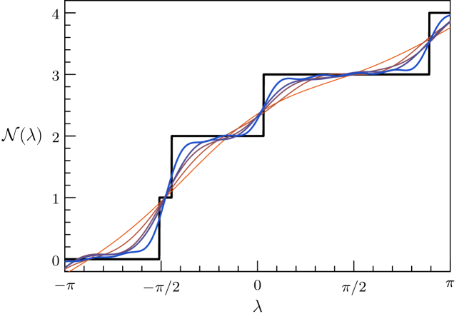
Figure 1: Spectral counting function $\mathcal{N}(\lambda)$ for a Hermitian $4\times 4$ matrix $H$ with eigenvalues $\lambda_{1}=-1.6$, $\lambda_{2}=-1.4$, $\lambda_{3}=0.1$, and $\lambda_{4}=2.8$ (thick line) together with approximations at finite resolution $\epsilon>0$ based on the trace formula (10). The five approximations correspond to a cut-off $n_{\mathrm{max}}$ taking values in $\{2,3,4,5,10\}$, $s_{\mathrm{max}}=9n_{\mathrm{max}}$ and resolution $\epsilon=1/n_{\mathrm{max}}$.

Appendix B Some relations following from the Worpitzky identity

The Worpitzky identity (42) can be used to derive many identities involving the Eulerian numbers. Below we derive a few and use them to prove the identity (48).

Let us start by substituting $z=\pm r$ with $r\in\mathbb{Z}^{+}$ and $r<s$ in the Worpitzky identity (42). We get two sets of identities by removing all the terms in the product which include a vanishing factor. This gives

$$\sum_{k=s-r}^{s-1}A(s,k)\left(\begin{array}[]{c}k+r\\ s\end{array}\right)=r^{s}\ ,$$ (108)

and

$$\sum_{k=0}^{r-1}A(s,k)\left(\begin{array}[]{c}r+s-k-1\\ s\end{array}\right)=r^{s}\ .$$ (111)

Other identities are obtained by first writing the binomial coefficients in (42) as a polynomial of degree $s$ in the variable $z$

$$\binom{z+k}{s}=\prod_{l=1}^{s}(z+k+1-l)=\sum_{j=0}^{s}\alpha_{j}(s,k)z^{j}$$ (112)

where $\alpha_{j}(s,k)$ are the coefficients of this polynomial. Then (42) reads

$$\sum_{j=0}^{s}z^{j}\,\left[\sum_{k=0}^{s-1}A(s,k)\alpha_{j}(s,k)\right]=s!z^{s}$$ (113)

Hence, all the coefficients in the polynomial on the left hand side must vanish, except for the $j=s$ one for which, using (23) one finds $\alpha_{s}(s,k)=1$.
Denoting $t_{r}=\sum_{q=1}^{s}(k+1-q)^{r}$, the Newton identities enable one to write

$$\alpha_{s-m}{(s,k)}=\frac{1}{m!}\left|\begin{array}[]{ccccc}t_{1}&1&0&\cdots&0\\ t_{2}&t_{1}&2&\cdots&0\\ \vdots&\vdots&\ddots&\ddots&\vdots\\ t_{m-1}&t_{m-2}&\cdots&t_{1}&m-1\\ t_{m}&t_{m-1}&\cdots&t_{2}&t_{1}\end{array}\right|.$$ (114)

The terms for $j=0$ vanishes identically since $\alpha_{0}(s,k)=\prod_{m=1}^{s}(k+1-m)=0\ \ \forall\ 0\leq k\leq s-1$. The next simple identities are obtained for $j=1\ {\rm and}\ j=s-1$ :

$$j=1:\qquad\quad \sum_{k=0}^{s-1}A(s,k)\left(\prod_{m\neq k+1}^{s}(k+1-m)\right) =$$

$$\sum_{k=0}^{s-1}A(s,k)(-1)^{s-1-k}k!(s-1-k)! =0\ ,$$ (115a)

$$\qquad j=s-1:\qquad\quad \sum_{k=0}^{s-1}A(s,k)\left((k+1)s-\frac{s(s+1)}{2}\right) =0\ .\qquad\qquad\quad$$ (115b)

Further identities can be written by expressing the $\alpha_{j}{(s,k)}$ explicitly.

In the rest of this appendix we derive the identity (48). Let us start by introducing

$$B^{(m)}(s,k)=\left[\frac{d^{s}}{dz^{s}}\left(z^{k}(\log z)^{m}\right)\right]_{z=1}$$ (116)

as a short-hand for the expression in the square brackets in identity (48). This can be computed to give

$$B^{(m)}(s,k)= s!(-1)^{m}\sum_{l=\mathrm{max}(s-k,m)}^{s}(-1)^{l}\begin{pmatrix}k\\ s-l\end{pmatrix}\sum_{\underline{j}\in\mathcal{P}(k,l)}\left(\prod_{i=1}^{k}j_{i}\right)^{-1}\ ,$$ (117)

where, $\mathcal{P}(k,l)$ is the set of partitions of $l$ to $k$ integers $(j_{1},j_{2},\cdots,j_{k})\doteq\underline{j}$, and all the $j_{i}$ are positive definite, with $\sum_{i=1}^{k}j_{i}=l$. It is easy to show that $B^{m}(m,k)=m!\forall\ m-1\geq k\geq 0$, which together with (23) satisfies (48) for $s=m$. Next let us prove the identity

$$B^{(m)}(s,k)=\frac{\alpha_{m}(s,k)}{m!}$$ (118)

which will lead directly to (48). To show (118) substitute $z=e^{x}$ in (116) so that

$$B^{(m)}(s,k)=\left[(e^{-x}\frac{d}{dx})^{s}e^{kx}x^{m}\right]_{x=0}\ .$$ (119)

Next define the generating function

$$F(s,k;y)=\sum_{m=0}^{\infty}B^{(m)}(s,k)\frac{y^{m}}{m!}\ ,$$ (120)

substitute (119) and sum to obtain

$$F(s,k;y)=\binom{k+y}{s}$$ (121)

which is exactly the polynomial whose coefficients are the $\alpha_{j}(s,k)$ as defined above. This proves (48).

Appendix C Examples

For illustration we work out explicitly the discrete-time quantum evolution operator $S_{II}(\lambda)$ and the corresponding spectral determinant $\zeta_{II}(\lambda,z)$ if the underlying graph is either an interval (the complete graph with $N=2$ vertices) or a 2-star (equivalently, a chain of $N=3$ vertices).

C.1 The interval ($N=2$)

For a Hermitian $2\times 2$ matrix $H$ with $H_{12}\neq 0$ the corresponding graph is just a single interval and the quantum evolution operator takes the form

$$S_{II}(\lambda)=\begin{pmatrix}0&\sigma^{(2)}_{11}(\lambda)\\ \sigma^{(1)}_{22}(\lambda)&0\end{pmatrix}$$ (122)

where $\sigma^{(1)}_{22}(\lambda)$ and $\sigma^{(2)}_{11}(\lambda)$ are unimodular scattering phases

$$\sigma^{(1)}_{22}(\lambda) =i\frac{H_{11}-\lambda+ih_{12}}{H_{11}-\lambda-ih_{12}}=i\frac{(H_{11}-\lambda)^{2}-|H_{12}|^{2}+2ih_{12}(H_{11}-\lambda)}{(H_{11}-\lambda)^{2}+|H_{12}|^{2}}$$ (123)

$$\sigma^{(2)}_{11}(\lambda) =i\frac{H_{22}-\lambda+ih_{12}}{H_{22}-\lambda-ih_{12}}=i\frac{(H_{22}-\lambda)^{2}-|H_{12}|^{2}+2ih_{12}(H_{22}-\lambda)}{(H_{22}-\lambda)^{2}+|H_{12}|^{2}}\ .$$ (124)

The determinant is given by

$$\begin{split}\mathrm{det}\,\left(S_{II}(\lambda)\right)=&-\sigma^{(1)}_{22}(\lambda)\sigma^{(2)}_{11}(\lambda)\\ =&\frac{\zeta_{H}(\lambda)+ih_{12}\left(H_{11}+H_{22}-2\lambda\right)}{\zeta_{H}(\lambda)-ih_{12}\left(H_{11}+H_{22}-2\lambda\right)}\end{split}$$ (125)

and the spectral determinant is

$$\zeta_{II}(\lambda,z)=1-z^{2}\sigma^{(1)}_{22}(\lambda)\sigma^{(2)}_{11}(\lambda)=\left(1-z\sqrt{\sigma^{(1)}(\lambda)\sigma^{(2)}(\lambda)}\right)\left(1+z\sqrt{\sigma^{(1)}(\lambda)\sigma^{(2)}(\lambda)}\right)$$ (126)

which is consistent with the fact that the two eigenvalues of $S_{II}(\lambda)$ (which can be read directly from the matrix itself) are

$$\begin{split}z_{1}=e^{i\theta_{1}(\lambda)}=&\sqrt{\sigma^{(1)}_{22}(\lambda)\sigma^{(2)}_{11}(\lambda)}\\ z_{2}=e^{i\theta_{2}(\lambda)}=&-\sqrt{\sigma^{(1)}_{22}(\lambda)\sigma^{(2)}_{11}(\lambda)}\end{split}\ .$$ (127)

Rewriting the spectral determinant as

$$\zeta_{II}(\lambda,z)=1-z^{2}+z^{2}\zeta_{II}(\lambda)$$ (128)

with

$$\zeta_{II}(\lambda)=\frac{2\zeta_{H}(\lambda)}{\left(H_{11}-\lambda-ih_{12}\right)\left(H_{22}-\lambda-ih_{12}\right)}$$ (129)

shows that $\zeta_{II}(\lambda)$ has the same zeros as $\zeta_{H}(\lambda)$ in the complex $\lambda$-plane.

C.2 The two-star graph ($N=3$)

Next consider the Hamiltonian of the form

$$H=\begin{pmatrix}H_{11}&H_{12}&H_{13}\\ H_{21}&H_{22}&0\\ H_{31}&0&H_{33}\end{pmatrix}.$$ (130)

This corresponds to a two-star graph with the central vertex $v=1$ of degree $d_{1}=2$ and two vertices $v=2$ and $v=3$ of degree one. The spectral determinant of the Hamiltonian is then

$$\zeta_{H}(\lambda)=\left(H_{11}-\lambda\right)\left(H_{22}-\lambda\right)\left(H_{33}-\lambda\right)-\left(H_{22}-\lambda\right)|H_{13}|^{2}-\left(H_{33}-\lambda\right)|H_{12}|^{2}\ .$$ (131)

With $\Gamma_{1}=h_{12}+h_{13}\equiv|H_{12}|+|H_{13}|$ the corresponding vertex scattering matrices are

$$\begin{split}\sigma^{(1)}=&\frac{i}{H_{11}-\lambda-i\Gamma_{1}}\begin{pmatrix}\left(H_{11}-\lambda+i(h_{12}-h_{13})\right)&i2\sqrt{h_{12}h_{13}}e^{i(\gamma_{13}-\gamma_{12})}\\ i2\sqrt{h_{12}h_{13}}e^{-i(\gamma_{13}-\gamma_{12})}&\left(H_{11}-\lambda+i(h_{13}-h_{12})\right)\end{pmatrix}\\ \sigma^{(2)}\equiv&\sigma^{(2)}_{11}=i\frac{H_{22}-\lambda+ih_{12}}{H_{22}-\lambda-ih_{12}}\\ \sigma^{(3)}\equiv&\sigma^{(3)}_{11}=i\frac{H_{33}-\lambda+ih_{13}}{H_{33}-\lambda-ih_{13}}\ .\end{split}$$ (132)

The quantum evolution operator has the form

$$S_{II}(\lambda)=\begin{pmatrix}0&0&\sigma^{(2)}_{11}&0\\ 0&0&0&\sigma^{(3)}_{11}\\ \sigma^{(1)}_{22}&\sigma^{(1)}_{23}&0&0\\ \sigma^{(1)}_{32}&\sigma^{(1)}_{33}&0&0\end{pmatrix}$$ (133)

and has determinant

$$\mathrm{det}\,\ S_{II}(\lambda)=\sigma^{(2)}_{11}\sigma^{(3)}_{11}\mathrm{det}\,\ \sigma^{(1)}=\prod_{v=1}^{3}\frac{H_{vv}-\lambda+i\Gamma_{v}}{H_{vv}-\lambda-i\Gamma_{v}}=\frac{G(\lambda)+iF(\lambda)}{G(\lambda)-iF(\lambda)}$$ (134)

where

$$\begin{split}G(\lambda)=&\mathrm{Re}\left(\prod_{v=1}^{3}(H_{vv}-\lambda+i\Gamma_{v})\right)\\ =&\zeta_{H}(\lambda)-\Gamma_{2}\Gamma_{3}\mathrm{tr}(H-\lambda)\\ F(\lambda)=&\mathrm{Im}\left(\prod_{v=1}^{3}(H_{vv}-\lambda+i\Gamma_{v})\right)\\ =&(H_{22}-\lambda)(H_{11}+H_{33}-2\lambda)\Gamma_{3}+(H_{33}-\lambda)(H_{11}+H_{22}-2\lambda)\Gamma_{2}-\Gamma_{1}\Gamma_{2}\Gamma_{3}\end{split}$$ (135)

The spectral determinant can be calculated by direct calculation as

$$\begin{split}\zeta_{II}(\lambda,z)=&1+z^{2}\frac{2\zeta_{H}(\lambda)+2\Gamma_{2}\Gamma_{3}\mathrm{tr}\left(H-\lambda\right)}{(H_{11}-\lambda-i\Gamma_{1})(H_{22}-\lambda-i\Gamma_{2})(H_{33}-\lambda-i\Gamma_{3})}+z^{4}\mathrm{det}\,\ S_{II}(\lambda)\\ =&\frac{\zeta_{H}(\lambda)\left(1+z^{2}\right)^{2}-\Gamma_{2}\Gamma_{3}\mathrm{tr}\left(H-\lambda\right)\left(1-z^{2}\right)^{2}+i(z^{4}-1)F(\lambda)}{\prod_{v=1}^{3}\left(H_{vv}-\lambda-i\Gamma_{v}\right)}\ .\end{split}$$ (136)

At $z=1$ this reduces to

$$\zeta_{II}(\lambda)=\frac{4\zeta_{H}(\lambda)}{\prod_{v=1}^{3}\left(H_{vv}-\lambda-i\Gamma_{v}\right)}\ .$$ (137)

Note that the spectral determinant $\zeta_{II}(\lambda,z)$ is bi-quadratic and the zeros can be calculated directly as

$$\begin{split}z_{n}=&e^{i\theta_{n}(\lambda)}\\ =&\pm i\sqrt{\frac{\zeta_{H}(\lambda)+\Gamma_{2}\Gamma_{3}\mathrm{tr}(H-\lambda)\pm i\sqrt{\prod_{v=1}^{3}|H_{vv}-\lambda+i\Gamma_{v}|^{2}-\left(\zeta_{H}(\lambda)+\Gamma_{2}\Gamma_{3}\mathrm{tr}(H-\lambda)\right)^{2}}}{\prod_{v=1}^{3}(H_{vv}-\lambda+i\Gamma_{v})}}\end{split}$$ (138)

where $n\in\{1,2,3,4\}$ refers to the 4 different choices of signs.

References

- (1) A. Selberg, Harmonic analysis and discontinuous groups in weakly symmetric Riemannian spaces with applications to Dirichlet series, J. Indian Math. Soc. (N.S.) 20, 47-87 (1956).
- (2) M.C. Gutzwiller, Energy spectrum according to classical mechanics, J. Math. Phys. 11, 1791 (1970).
- (3) M.C. Gutzwiller (1971). Periodic Orbits and Classical Quantization Conditions , J. Math. Phys. 12, 343 (1971).
- (4) M.C. Gutzwiller, Chaos in Classical and Quantum Mechanics (1990, Springer, New York).
- (5) R. Balian, C. Bloch, Solution of the Schrödinger equation in terms of classical paths, Ann. Physics 85, 514 (1974).
- (6) M.V. Berry, M. Tabor, Closed orbits and the regular bound spectrum, Proc. R. Soc. Lond. A 349, 101 (1976).
- (7) A.M. Ozorio de Almeida, Hamiltonian Systems: Chaos and Quantization (Cambridge University Press, 1989).
- (8) F. Haake, S. Gnutzmann, M. Kuś, Quantum Signatures of Chaos (4th edition, Springer, 2018)
- (9) E. Wigner, On the Distribution of the Roots of Certain Symmetric Matrices, Ann. of Math. 67, 325-328 (1958).
- (10) U. Smilansky, Quantum chaos on discrete graphs, J. Phys. A, 40, F621-F630 (2007).
- (11) I. Oren, A. Godel, U. Smilansky, Trace formulae and spectral statistics for discrete Laplacians on regular graphs (I), J. Phys. A 42, 415101 (2009).
- (12) I. Oren, U. Smilansky, Trace formulae and spectral statistics for discrete Laplacians on regular graphs (II), J. Phys. A 43, 225205 (2010).
- (13) Y. Ihara, Discrete subgroups of , pages 272-278 in A. Borel, G. Mostow (editors) Algebraic Groups and Discontinuous Subgroups (AMS, Providence, R.I., 1966).
- (14) Y. Ihara, On discrete subgroups of the two by two projective linear group over p-adic fields, J. Math. Soc. Japan, 18,219–235 (1966).
- (15) K. Hashimoto, Zeta functions of finite graphs and representations of p-adic groups, pages 211-280 in: K. Hashimoto, Y. Namikawa (editors),Automorphic forms and geometry of arithmetic varieties, (Adv. Stud. Pure Math. volume 15, Academic Press, Boston, 1989).
- (16) K. Hashimoto, A. Hori, Selberg-Ihara’s zeta function for p-adic discrete groups, pages 171-210 in: K. Hashimoto, Y. Namikawa (editors),Automorphic forms and geometry of arithmetic varieties, (Adv. Stud. Pure Math. volume 15, Academic Press, Boston, 1989).
- (17) K. Hashimoto, On zeta and L-functions of finite graphs, Internat. J. Math. 1, 381-396 (1990).
- (18) K. Hashimoto, Artin type L-functions and the density theorem for prime cycles on finite graphs, Internat. J. Math. 3,809-826 (1992).
- (19) H. Bass, The Ihara-Selberg zeta function of a tree lattice, Internat. J. Math., 3, 717-797 (1992).
- (20) L. Bartholdi, Counting paths in graphs, Enseign. Math., 45, 83-131 (1999).
- (21) M. Kotani, T. Sunada, Zeta functions of finite graphs, J. Math. Sci. Univ. Tokyo 7,7-25 (2000).
- (22) N. Anantharaman, Some relations between the spectra of simple and non-backtracking random walks, arXiv:1703.03852 [math.PR] (2017)
- (23) L. Euler, Memoires de l’academie des sciences de Berlin 17, 1768, 83-106 (1768).
- (24) J. Worpitzky, Studien über die Bernouillischen und Eulerischen Zahlen, J. reine angew. Math. 94, 203-232, (1883).
- (25) M.L. Mehta, Random Matrices (3rd edition, Academic Press, 2004).
- (26) P.J. Forrester, Log-Gases and Random Matrices (Princeton University Press, 2010).
- (27) I. Dumitriu, A. Edelman, Matrix models for beta ensembles, J. Math. Phys. 43, 5830 (2006).
- (28) E. Wigner, Characteristic vectors of bordered matrices with infinite dimensions, Ann. Math. 62, 548-564 (1955).
- (29) M. Ledoux, A recursion formula for the moments of the Gaussian orthogonal ensemble, Annales de l’Institut Henri Poincaré 45, 754-769 (2009).
- (30) S. Gerschgorin, Über die Abgrenzung der Eigenwerte einer Matrix, (in german), Izv. Akad. Nauk. USSR Otd. Fiz.-Mat. Nauk 6, 749-754 (1931).
- (31) C. Mahaux, H.A. Weidenmüller, Shell Model Approach in Nuclear Reactions (North-Holland, Amsterdam, 1969).
- (32) D. Waltner, S. Gnutzmann, G. Tanner, K. Richter, Subdeterminant approach for pseudo-orbit expansions of spectral determinants in quantum maps and quantum graphs Phys. Rev. E 87, 052919 (2013).
- (33) R. Band, J.M. Harrison, C.H. Joyner, Finite pseudo orbit expansions for spectral quantities of quantum graphs, J. Phys. A 45, 325204 (2012).
- (34) S. Gnutzmann, U. Smilansky, Quantum Graphs: Applications to Quantum Chaos and Universal Spectral Statistics, Advances in Physics 55, 527 (2006).
- (35) J. Kempe, Quantum random walks: An introductory overview, Contemporary Physics, 44, 307-327 (2003).
- (36) H. Schanz, U. Smilansky, Periodic-orbit theory of Anderson localization on graphs. Phys. Rev. Lett. 84, 1427-1430 (2000).