Bifurcations of autoresonant modes in oscillating systems with combined excitation
Abstract. A mathematical model describing the capture of nonlinear systems into the autoresonance by a combined parametric and external periodic slowly varying perturbation is considered. The autoresonance phenomenon is associated with solutions having an unboundedly growing amplitude and a limited phase mismatch. The paper investigates the behaviour of such solutions when the parameters of the excitation pass through bifurcation values. In particular, the stability of different autoresonant modes is analyzed and the asymptotic approximations of autoresonant solutions on asymptotically long time intervals are proposed by a modified averaging method with using the constructed Lyapunov functions.
Keywords: nonlinear equations, autoresonance, asymptotics, stability, bifurcation
Mathematics Subject Classification: 34C23, 34 29, 34D05, 37B25, 37B55
Introduction
Autoresonance is a phenomenon that occurs when a nonlinear oscillating system is perturbed by a slowly varying periodic force. Under certain initial conditions, the system automatically adjusts to the pumping and keeps this state for a sufficiently long period of time. Due to this effect, the energy of the system can increase significantly [1, 2]. The autoresonance was first suggested in the problems associated with the acceleration of relativistic particles in the middle of the twentieth century, and nowadays it is considered as a universal phenomenon that plays the important role in a wide range of physical systems [3, 4, 5, 6, 7]. The study of relevant mathematical models leads to new and interesting problems in the field of nonlinear dynamics [8, 9, 10, 11].
Mathematical models associated with the autoresonance have been actively studied recently. In particular, the models with the external driving were investigated in [12, 8], while the systems with the parametric pumping were considered in [13, 14]. Much less attention was paid to the systems with a combined external and parametric excitation. In particular, it was shown in [15] that the combined excitation leads to the coexisting of several stable autoresonant modes with different phase mismatches depending on the values of the excitation parameters. In this paper, the autoresonance model with the combined excitation is considered and the behaviour of its solutions in the vicinity of bifurcation points is investigated.
The paper is organized as follows. In section 1, the mathematical formulation of the problem is given. In section 2, the autoresonant modes are described and the partition of a parameter space is constructed. In section 3, the stability of different particular autoresonant solutions is discussed. Section 4 provides asymptotic analysis of general autoresonant solutions using the constructed Lyapunov functions. A discussion of the results obtained is contained in section 5.
1. Problem statement
Consider the non-autonomous system of two nonlinear differential equations [15]:
| (1) | ||||
with the parameters , and a smooth given function . This system arises in the study of the autoresonance phenomena for a wide class of nonlinear oscillators with the combined parametric and external chirped-frequency excitation. The solutions and correspond to the amplitude and the phase mismatch of the nonlinear oscillators. The solutions to system (1) with and as are associated with the phase-locking and the capture into the autoresonance, while the solutions with and as relate to the phase-slipping phenomenon and the absence of the capture.
The joint influence of the parametric and the external excitations is determined by the behaviour of the function . Indeed, if , , the parametric pumping is weak and system (1) corresponds to a perturbation of the model with the pure external excitation [12]. If , the external driving becomes insignificant and system (1) represents a perturbation of the model of parametric autoresonance [16]. The parametric and the external excitations act equally only when . In this paper it is assumed that
Note that system (1) appears when the long-term evolution of perturbed nonlinear systems is investigated by using the averaging method [17]. A simple example is given by the following equation:
| (2) |
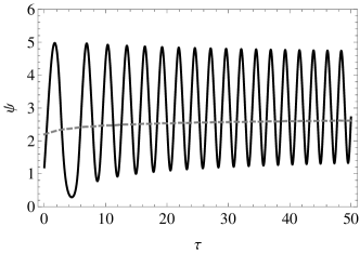
where , , , , . It is easy to see that equation (2) with has the stable solution . Solutions to (2) with initial values sufficiently close to the equilibrium , whose the energy increases significantly with time and the phase is synchronized with pumping such that , are associated with the capture into the autoresonance. To approximate such solutions, introduce slow and fast variables: and , where . Then the substitution
into equation (2) and the averaging over the fast variable give system (1) for the functions and with and . A similar but more complex transition to system of type (1) takes place when studying of autoresonant energy excitation in infinite-dimensional systems described by nonlinear partial differential equations (see, for instance, [9]).
It follows from [15] that system (1) admits two or four autoresonant modes with different phase mismatches. The number of modes and their stability depend on the values of the parameters , , and . It was shown that the transition of these parameters through critical values can lead to stabilization or losing the stability of the autoresonant solutions via a non-autonomous version of the centre-saddle bifurcation [18]. The behaviour of the autoresonant solutions near the bifurcation points has not been discussed previously. In this paper the stability and the long-term asymptotics for such solutions are investigated.
In the first step, particular autoresonant solutions with unboundedly growing amplitude having power-law asymptotics at infinity are considered, and the partition of a parameter plane is outlined. Then, the stability of the particular solutions is discussed at the bifurcation points. The stability of some solutions can be investigated by trivial linear analysis failing in the study of the other ones, where nonlinear terms of equations must be considered. The stability of these solutions is analysed by constructing of suitable Lyapunov functions. The presence of stability ensures the existence of a family of autoresonant solutions with a similar asymptotic behaviour. In the last step, the asymptotic behaviour of such solutions is analyzed.
2. Particular autoresonant solutions
The asymptotics for the particular solutions , with the unbounded amplitude and the bounded phase mismatch are constructed in the form of power series with constant coefficients:
| (3) |
The substitution these series into system (1) and the grouping the terms of the same power of lead to finding the coefficients , , and , where is one of the roots to the following equation:
| (4) |
The last equation has a different number of roots depending on the values of and . If the inequality holds, all the remaining coefficients , as are determined from the chain of linear equations:
| (5) | ||||
where , ,
etc. In particular,
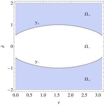
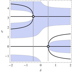
The pair of the equations and defines the bifurcation curves
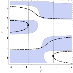
in the parameter plane , where . It can easily be checked that system (5) is solvable whenever . The bifurcation curves divide the parameter plane into the following parts (see Fig. 1):
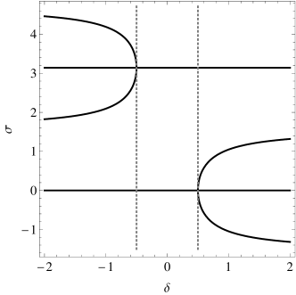
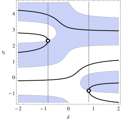
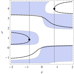
If , the equation has four different roots. In the case , there are only two different roots (see Fig. 2).
Theorem 1 (see [15]).
2.1. The roots of multiplicity 2
If , there exists such that and . In addition, suppose that , then is the root of multiplicity 2. In this case, system (5) is unsolvable and the solution cannot be constructed in the form of (3). The asymptotic solutions are sought in the form
| (6) |
Substituting the series in system (1) and equating the terms of the same power of , we get , and
| (7) |
Since , it follows that the asymptotic solution in the form (6) does not exist when . If , equation (7) has two different roots:
The remaining coefficients , as are determined from the following recurrent system of equations:
where ,
etc.
2.2. The roots of multiplicity 3
Now suppose and is the root of equation (4) such that and . These imply that , and . In this case, the asymptotic solutions are constructed in the following form:
| (8) |
It can easily be checked that
The remaining coefficient , as are determined from the following chain of equations:
where ,
etc.
3. Stability analysis
3.1. Linear analysis
Let , be one of the particular autoresonant solutions with asymptotics (3), (6) or (8). The substitution , into (1) gives the following system with a fixed point at :
| (9) | ||||
Consider the linearized system:
Define
for , where is one of the roots to equation (4). Then the functions and have the following asymptotics as : and
-
•
if is the simple root,
-
•
if is the root of multiplicity 2,
-
•
if is the root of multiplicity 3.
Then the roots of the corresponding characteristic equation can be represented in the form
where
as and . Therefore, if is the simple root of (4) such that , the leading asymptotic terms of are real of different signs:
This implies that the fixed point of (9) is a saddle in the asymptotic limit, and the corresponding solutions , to system (1) are unstable. Similarly, if is the root of multiplicity 2 such that and , , then
In this case the fixed point of (9) and the corresponding particular solution to system (1) are both unstable. In the same way, the fixed point of the linearized system is unstable when is the root of multiplicity 3 and . In this case, the eigenvalues have the following asymptotics:
Thus we have
Theorem 3.
Let us consider the following three cases that are not covered by Theorem 3:
- Case I:
-
.
- Case II:
-
, and as .
- Case III:
-
, , and .
In these cases, the roots of the characteristic equation are complex. In particular,
and as . In all three cases, the fixed point of system (9) is a centre in the asymptotic limit. Note that the linear stability analysis fails when as (see [22, 23, 15]), and the nonlinear terms of the equations must be taken into account.
3.2. Lyapunov functions
When linear stability analysis does not work, Lyapunov’s method can be applied. This method assumes the existence of a locally positive definite function with a sign definite derivative along the trajectories of the system. The sign of the derivative determines whether the solution is stable or unstable. Although this method is well-developed, there is no systematic way to find appropriate Lyapunov functions. In this section, we construct such functions to prove the stability or the instability of the autoresonant solutions in different cases.
Theorem 4.
Proof.
Let be a one of the particular solutions with power-law asymptotics at infinity. The change of variables
transforms system (1) into the form
| (10) |
where
and
In the new variables , the system has equilibrium at the origin . Note that a key role in the stability analysis is played by the asymptotic behaviour of the right hand sides of the equations as plays. Taking into account the asymptotic formulas for the particular solutions and , we obtain
and
as and for all , where
Note that these asymptotic formulas depend on the choice of the particular solution to system (1) and the root of equation (4).
Consider Case I, when is the simple root to equation (4) and the particular solution has asymptotics (3). Hence as , and we get
where
In this case, the combination
| (11) |
is used as a Lyapunov function candidate for system (10), where
Note that the functions , , and have the following asymptotics:
as and , where . The asymptotic estimates are uniform with respect to in the domain , where , . Then for all there exist and such that
for all , where
Note that the combination of the functions , , and has the sign definite total derivative with respect to . Indeed, it can easily be checked that
Summing up the last expressions, we obtain
as and . Hence, for all there exist and such that
| (12) |
for all . Thus, for all there exist such that
for all , where and . The last estimates and the negativity of the total derivative of the function ensure that any solution of system (10) with initial data cannot leave the domain as . Hence, the fixed point is stable as . The stability on the finite time interval follows from the theorem on the continuity of the solutions to the Cauchy problem with respect to the initial data.
Consider Case II. Let be a root of multiplicity 2 to equation (4) such that and . In this case, the particular solution , has the asymptotics (6) and as . Hence,
as and . Since the function is sign indefinite, the combination (11) can not be used as a Lyapunov function candidate.
Consider the change of variables
in system (10). The transformed system is
| (13) |
where
Taking into account (6), it can easily be checked that
as and for all , where
, as , and . We see that the function is suitable for the basis of a Lyapunov function candidate. Consider the following combination:
| (14) |
It is easy to prove that for all there exist and such that
for all , where
It turns out that the total derivative of the function has a sign definite leading term of the asymptotics:
| (15) | ||||
as and . Hence, for all there exist and such that
| (16) |
for all . The last inequality implies the instability of the equilibrium to system (13). Indeed, let be a solution to system (13) with initial data and such that , where , , and . By integrating (16) with respect to , we obtain the following inequality:
as . Hence, there exists such that the solution , escapes from the domain as . This means that the equilibrium is unstable. Returning to the original variables , we obtain the result of the theorem.
Finally, consider Case III. Let be a root of multiplicity 3 to equation (4) such that and . Then the solution , has the asymptotics (8), and . In this case,
as and . Note that this function can not be used in the construction of a Laypunov function. Indeed, if is small enough and is big enough (for example, and , where ), the leading and the remainder terms in the last expression can be of the same order. Hence the function is sign indefinite in a neighborhood of the equilibrium.
Consider the change of variables
in system (10). It can easily be checked that the transformed system has the form
| (17) |
where
Using asymptotic formulas for the particular solution, we obtain
as and for all , where . Consider the combination
as a Lyapunov function candidate for system (17). It follows easily that for all there exist and such that
for all , where
The derivative of this function with respect to along the trajectories of system (17) has the following asymptotics:
as and . Hence, for all there exist and such that
| (18) |
for all . The last inequality implies that the fixed point of system (17) is unstable. Indeed, let , be a solution to system (17) with initial data , such that , where , , and . Integrating (18) with respect to yields
as . Hence there exists such that the solution , escapes from the domain as . Thus, the fixed point of system (10) and the particular solution , to system (1) are unstable. ∎
Thus, the particular autoresonant solutions with power-law asymptotics are unstable (with respect to all the variables) in Case II and Case III. However, due to weak instability, it can be shown that there is a partial stability [24] with respect to one of the variables on an asymptotically long time interval. We have the following.
Theorem 5.
Proof.
Consider the change of variables
| (19) |
in system (10). It is clear that the system for the new variables has the following form:
| (20) |
where
Furthermore, using asymptotic formulas for the solution , , we get
as and for all . Note that there exists such that for every , the Hamiltonian is a positive definite quadratic form in the vicinity of the fixed point . Consider the following perturbation of as a Lyapunov function candidate for system (20):
where
Note that for all there exist and such that
for all and , where
The derivatives of functions and with respect to along the trajectories of system (20) have the following asymptotics:
as and . Combining the last expressions, we see that
Hence, for all there exist and such that
| (21) |
for all and . Besides, for all there exist such that
for all , where , , , and . This implies that any solution of system (20) starting in at satisfies the inequalities:
as . Hence, the equilibrium of system (20) is -stable at least on the asymptotically long time interval. Returning to the original variables , we obtain the result of the theorem. ∎
Similarly, we have the following.
Theorem 6.
Proof.
The change of variables
| (22) |
transforms system (10) into
| (23) |
where
By taking into account the asymptotics for the particular solution, we obtain
as . As above, we use the Hamiltonian as the basis for the Lyapunov function. Consider the combination:
where
It follows easily that for all there exist and such that
for all and , where
Calculating the derivatives of the functions and with respect to along the trajectories of system (23), we obtain
as and . Combining the preceding estimates, we get
Hence, for all there exist and such that
| (24) |
for all and . Therefore, as in the previous case, the fixed point of system (23) is -stable on an asymptotically long time interval: for all there exists such that any solution of system (23) starting from at satisfies the inequalities
as , where and . Returning to the original variables, we see that the particular solution , is -stable on the asymptotically long time interval.
∎
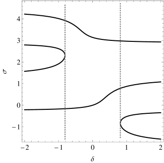
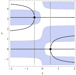
The stability of the particular solutions , ensures the existence of a family of autoresonant solutions with a similar behaviour (see Fig. 3). Some rough estimates for these solutions follow directly from the properties of constructed Lyapunov functions.
We have the following.
Corollary 1.
For all there exist and such that for all : the solution , to system (1) with initial data , has the following estimates:
| (25) | ||||
| (26) | ||||
| (27) |
Proof.
Let us fix . Consider Case I. Let , be a solution to system (10) starting from the ball at , where and (see Theorem 4). Then it follows from (12) that the function satisfies the inequality:
as , where . Integrating the last expression with respect to , we obtain , where , . Thus we have as . Returning to the original variables , we derive (25).
Consider Case II. Let , be a solution to system (20) starting from at , where , (see Theorem 5). From (21) it follows that the derivative of the function satisfies the following inequality:
as . By integrating the last estimate with respect to , we get , where , . Hence, as . The change of variables (19) transforms the last estimate into (26).
Finally, consider Case III. Let , be a solution to system (23) with initial data from the domain at , where and (see Theorem 6). From (24) it follows that the function satisfies the inequality:
as . As in the previous case, by integrating the last inequality, we obtain , where , . Hence, as . Combining this with (22), we get (27). ∎
4. Asymptotic analysis
In this section, the asymptotics for general autoresonant solutions starting from a neighborhood of stable solutions are specified by a modified averaging method [17, 25, 26, 27] with using the constructed Lyapunov functions.
Asymptotics are most simply constructed in Case I, when is a simple root to equation (4). We have the following (see [15]).
Theorem 7.
In other cases, the stability of the particular solutions , has not been justified for all . Therefore, the asymptotics for general autoresonant solutions are constructed only on the asymptotically long time intervals.
Theorem 8.
Let be a root of multiplicity 2 to equation (4). Then, in Case II, there exists such that a two-parameter family of autoresonant solutions , to system (1), starting at from -neighbourhood of the solution , , has the following asymptotics:
as uniformly for , where has the following form:
with , and as .
Proof.
Let , be a particular solution to system (1) with asymptotics (6), where . We apply the change of variables
in system (1) and study the solutions of transformed system (13) in a neighborhood of the unstable equilibrium . Consider the Hamiltonian system:
where
It is follows from the definition of the function that the level lines define a family of closed curves on the phase space parameterized by the parameter , . It can easily be checked that to each closed curve there corresponds a periodic solution , of period , where
These solutions are used in the definition of the functions
that are -periodic with respect to . Consider the change of variables
| (28) |
in system (13). Since
the transformation of variables (28) is reversible while . It can easily be checked that the system in the action-angle variables has the following form:
| (29) |
where
Note that and are -periodic functions with respect to such that
as and for all and . To simplify system (29), we introduce a new dependent variable associated with the Lyapunov function (14) such that
| (30) |
where is -periodic function in . It can easily be checked that as for all and . Hence, the transformation is reversible for all , and . The transformed system is given by
| (31) |
where
| (32) |
It is not difficult to deduce from (32) and (15) the asymptotics of the functions and at infinty:
where and are -periodic functions with respect to , and as for all . For the convenience, we rewrite system (31) in a near-Hamiltonian form:
| (33) |
where
The asymptotic solution to the first equation in (33) is sought in the form:
where is determined from the averaged equation
| (34) |
Then satisfies the equation:
| (35) |
with
In addition, it is assumed that is a -periodic function with zero average (with respect to ):
Equation (35) can be integrated with respect to by choosing the constant of integration in such a way that the result has a zero average:
| (36) |
The asymptotic solution to equation (36) is constructed in the form:
| (37) |
Substituting this series into equation (36) and equating the terms of the same power of , we obtain the following chain of equations:
where each function , is expressed through , , such that . For example,
Thus, all coefficients are uniquely determined in the class of -periodic functions with zero average .
In the same way, the solution to the second equation in (33) is sought in the form:
where is determined from the averaged equation
| (38) |
. The function satisfies the following equation:
| (39) |
where . The asymptotic solution to (39) is constructed in the form:
| (40) |
with the additional condition: . The substitution the series into equation (39) and the grouping the expressions of the same power of give the following chain of differential equations:
where each function for is expressed through , , . For example,
It follows easily that all coefficients are uniquely determined in the class of -periodic functions with .
In the last step, we integrate the averaged equations (34) and (38). First note that substituting series (37) and (40) for and in right-hand sides of the averaged equations, we get
as , where , , etc. Consider the following system of two differential equations:
| (41) |
. Since and , as , then every solution with initial data close to zero escapes from the domain at time . Note that the asymptotic approximation basing on the Lyapunov function is not valid as . Consider a one parametric family of solutions to the first equation in (41) with initial data , where is a small positive parameter. The asymptotic solution is sought in the form:
| (42) |
Substituting this into the equation and equating coefficients of powers of , we get , where as . Hence,
uniformly for . is found by integrating the second equation in (41) with respect to :
| (43) |
where is the arbitrary parameter: . Substituting (42) into (43), we obtain
uniformly for , where
as . Combining this with (37), (40), (42), (28) and (30), we get the following asymptotic approximation of solutions to system (13):
as uniformly for . Returning to the original variables we obtain the result of the theorem. ∎
Similarly, we have the following.
Theorem 9.
Let be a root of multiplicity 3 to equation (4). Then, in Case III, there exists such that a two-parameter family of autoresonant solutions , to system (1), starting at from -neighbourhood of the solution , , has the following asymptotics:
as uniformly for , where has the following form:
with , , as .
Proof.
The proof is similar to the proof of Theorem 8 with using the Lyapunov function instead of . ∎
5. Conclusion
In summary, the model of the autoresonant capture in nonlinear systems with the combined external and parametric excitation in the vicinity of the bifurcation points has been investigated. The suggested approach relies on the stability analysis of the particular solutions with power-law asymptotics at infinity. It has been shown that outside the bifurcation points there are several autoresonant modes with different phase shifts associated with simple roots to equation (4). Depending on the sign of the value , where , some of these modes are stable (see the shaded areas in Fig. 4). To each stable mode there corresponds the two-parameter family of the autoresonant solutions with the asymptotics detailed in Theorem 7. Some of the autoresonant modes coalesce, when the parameters passes through the bifurcation curves from to . Assume that equation (4) has only two different roots at the bifurcation point: is a root of multiplicity 3 and is a simple root. Then there are two autoresonant modes with different phase shifts. The stability of the mode corresponding to a multiple root depends on the sign of the value (see Theorem 6 and the shaded area in Fig. 5, a). In this case the stability has been justified on finite but asymptotically long time intervals. Now suppose that equation (4) has three different roots at the bifurcation point: is a root of multiplicity 2 and , are simple roots. Then system (1) has two or four autoresonant modes depending on the sign of value . In particular, in the case , there are two modes corresponding to the simple roots. In the opposite case, , there are two additional modes corresponding to and associated with the particular solutions having asymptotics (6). One of these additional modes with is stable on the asymptotically long time interval. The asymptotics for the general autoresonant solutions to system (1) at the bifurcation points has been described in Theorems 8 and 9.

Note that the stability of the particular autoresonant solutions have been justified by constructing the appropriate Lyapunov functions. These functions have been also used in the asymptotic analysis of the general solutions. In this approach the Lyapunov functions play the role of the action variable that usually appears in the study of the perturbed Hamiltonian systems by the averaging method. The using of the Lyapunov function as a new dependent variable simplifies considerably the construction of the asymptotic solutions to the perturbed non-autonomous systems and reveals the structure of the corresponding averaged equation at once.


It can easily be checked that system (1) rewritten in the form of (10) corresponds to a weak decaying perturbation of the autonomous system with the Hamiltonian that, in particular, arises in the study of a simple pendulum with vibrating suspension point. The bifurcations in this system have been discussed, for instance, in [28]. When the parameters of the unperturbed Hamiltonian system passes through the curves , the centre-saddle bifurcation occurs: the centre and the saddle coalesce or the additional pair of points (centre and saddle) appears from the stable or the unstable equilibrium (see Fig. 7 and 6). The presence of the time-dependent decaying perturbations in system (10) leads to a deformation of the phase portrait near the centres. In particular, some points become asymptotically (polynomially) stable, when the parameters are outside of the bifurcation curves. At the bifurcation points the centres corresponding to multiple roots of equation (4) become unstable with respect to all the variables. In this case the stability is preserved with respect to one of the variables at least on an asymptotically long time interval. Note that the bifurcations in non-autonomous systems of differential equations have been considered in several papers using different approaches [29, 30, 31]. However, to the best of our knowledge, the influence of general time-dependent decaying perturbations on the bifurcations of equilibria in Hamiltonian systems has not been thoroughly investigated. This will be discussed elsewhere.
Acknowledgements
The author is grateful to L.A. Kalyakin for useful discussions.
References
- [1] Fajans, J., Friedland, L.: Autoresonant (nonstationary) excitation of pendulums, Plutinos, plasmas, and other nonlinear oscillators. Amer. J. Phys. 69, 1096–1102 (2001)
- [2] Friedland, L.: Autoresonance in nonlinear systems. Scholarpedia. 4, 5473 (2009)
- [3] Neishtadt, A.I.: Autoresonance in electron cyclotron heating of a plasma. J. Exp. Theor. Phys. 66, 937–977 (1987)
- [4] Fajans, J., Gilson, E., Friedland, L.: Second harmonic autoresonant control of the l = 1 diocotron mode in pure electron plasmas. Phys. Rev. E. 62, 4131 (2000)
- [5] Barth, I., Friedland, L.: Quantum phenomena in a chirped parametric oscillator. Phys. Rev. Lett. 113, 040403 (2014)
- [6] Manfredi, G., Morandi, O., Friedland, L., Jenke, T., Abele, H.: Chirped-frequency excitation of gravitationally bound ultracold neutrons. Phys. Rev. D 95, 025016 (2017)
- [7] Batalov, S.V., Shagalov, A.G., Friedland, L.: Autoresonant excitation of Bose-Einstein condensates. Phys. Rev. E. 97, 032210 (2018)
- [8] Friedland, L.: Efficient capture of nonlinear oscillations into resonance. J. Phys. A. 41, 415101 (2008)
- [9] Kalyakin, L.A. Asymptotic analysis of autoresonance models. Russian Math. Surveys. 63, 791–857 (2008)
- [10] Neishtadt, A.I., Vasiliev, A.A., Artemyev, A.V.: Capture into resonance and escape from it in a forced nonlinear pendulum. Regul Chaot Dyn. 18, 686–696 (2013)
- [11] Glebov, S.G., Kiselev, O.M., Tarkhanov, N.: Nonlinear equations with small parameter. v. 1. Series in Nonlinear Analysis and Applications, 23, Oscillations and resonances. De Gruyter, Berlin (2017)
- [12] Kalyakin, L.A.: Asymptotic behavior of solutions of equations of main resonance. Theoret. and Math. Phys. 137, 1476–1484 (2003)
- [13] Khain, E., Meerson, B.: Parametric autoresonance. Phys. Rev. E. 64, 036619 (2001)
- [14] Kiselev, O.M., Glebov, S.G.: The capture into parametric autoresonance. Nonlinear Dynam. 48, 217–230 (2007)
- [15] Sultanov, O.: Stability and asymptotic analysis of the autoresonant capture in oscillating systems with combined excitation. SIAM J. Appl. Math. 78, 3103–3118 (2018)
- [16] Sultanov, O.A.: Stability of capture into parametric autoresonance. Proc. Steklov Inst. Math. 295 Suppl. 1, 156–167 (2016)
- [17] Bogolubov, N.N., Mitropolsky, Yu.A.: Asymptotic methods in theory of non-linear oscillations. Gordon and Breach, New York (1961)
- [18] Hanßmann, H.: Local and semi-local bifurcations in Hamiltonian systems - Results and examples. Lecture Notes in Mathematics 1893. Springer, Berlin (2007)
- [19] Kozlov, V.V., Furta, S.D.: Asymptotic solutions of strongly nonlinear systems of differential equations. Springer Monogr. Math. Springer, New York (2013)
- [20] Kuznetsov A.N.: Existence of solutions entering at a singular point of an autonomous system having a formal solution. Funct. Anal. Appl. 23, 308–317 (1989)
- [21] Kalyakin, L.A.: Existence theorems and estimates of solutions for equations of principal resonance. J. Math. Sci. 200, 82–95 (2014)
- [22] Thieme, H.: Asymptotically autonomous differential equations in the plane. Rocky Mountain J. Math. 24, 351–380 (1994)
- [23] Kalyakin, L.A., Sultanov, O.A.: Stability of autoresonance models. Differ. Equ. 49, 267–281 (2013)
- [24] Vorotnikov, V.I.: Partial stability and control. Birkhauser, Boston (1998)
- [25] Neishtadt, A.I.: The separation of motions in systems with rapidly rotating phase. J. Appl. Math. Mech. 48, 133–139 (1984)
- [26] Brüning, J., Dobrokhotov, S.Yu., Poteryakhin, M.A.: Averaging for Hamiltonian systems with one fast phase and small amplitudes. Math. Notes. 70, 599–607 (2001)
- [27] Arnold, V.I., Kozlov, V.V., Neishtadt, A.I.: Mathematical aspects of classical and celestial mechanics. Springer, Berlin (2006)
- [28] Neishtadt, A.I., Sheng, K.: Bifurcations of phase portraits of pendulum with vibrating suspension point. Commun Nonlinear Sci Numer Simulat. 47, 71–80 (2017)
- [29] Langa, J.A., Robinson, J.C., Suárez, A.: Stability, instability, and bifurcation phenomena in non-autonomous differential equations. Nonlinearity. 15, 887–903 (2002)
- [30] Kloeden, P.E., Siegmund, S.: Bifurcations and continuous transitions of attractors in autonomous and nonautonomous systems. Internat. J. Bifur. Chaos. 15, 743–762 (2005)
- [31] Rasmussen, M.: Bifurcations of asymptotically autonomous differential equations. Set-Valued Anal. 16, 821–849 (2008)