Chapter 0 Bursty Human Dynamics
1 Introduction
Bursty behaviour is a temporal character of some dynamical systems, which alternate between active periods with high frequency of events and long periods of inactivity. Dynamics characterised by such large temporal fluctuations cannot be explained by the conventional picture using Poisson processes assuming a single temporal scale, but rather can be the result of non-Poissonian dynamics inducing strong temporal heterogeneities on various temporal scales111Non-Poissonian bursty dynamics is in general characterised by the heterogeneous distribution of inter-event times passing between the consecutive occurrences of a given type of event. In contrast, in a system with Poissonian dynamics, inter-event times are distributed exponentially. However, many empirical inter-event time distributions are broad and follow a log-normal, Weibull, or power-law form, implying that the underlying mechanisms behind them maybe different than a Poisson process..
There are a number of systems in Nature that evolve following non-Poissonian dynamics [karsai2018bursty]. One example are earthquakes [corral2004longTerm, davidsen2013earthquake, bak2002unified, deArcangelis2006universality, smalley1987a], in which the times of shocks occurring at a given location show bursty temporal patterns, as illustrated in Fig. 1(a). Another example are solar flares with bursty emergence induced by huge and rapid releases of energy [mcAteer2007the, wheatland1998the]. It has been shown that the stochastic processes underlying these apparently different phenomena show such universal properties that lead to the same distributions of event sizes, inter-event times, and temporal clustering [deArcangelis2006universality], which can be arguably modelled by the frame of self-organised criticality (SOC) [bak1996how]. Burstiness is also seen in the contexts of neuronal systems where the firing of a single neuron (as shown in Fig. 1(b)) or collective of neurons appears with such dynamics [kemuriyama2010power]. Moreover, bursty patterns has been observed in ecology and animal dynamics in the context of initiating conflicts [proekt2012scale], communication, foraging [sorribes2011origin], predators waiting in ambush [wearmouth2014scaling], or the displacement of monkeys or mice [boyer2012nonrandom, nakamura2008of], which form complex self-similar temporal patterns reproduced on multiple time scales very similarly to examples observed in human behaviour. In addition, scale-invariant bursty temporal patterns have also been found in several man-made systems, like written text, in which successive occurrences of the same word display bursty patterns [altmann2009beyond]. In case of engineering systems perhaps some of the best examples are in the context of package-based traffic and wireless communication signals, which were found to evolve through non-Poissonian dynamics [chlebus1995is, janevski2003traffic, lee2013mobile, paxson1995wideArea]. Finally, financial markets, in which non-Poissonian dynamics characterises time series of returns of financial assets, stock sales, order books, and other transactions with dynamics studied in the realm of econophysics [mantegna2007introduction].

Bursty patterns have been found to characterise human dynamics in the timings of actions, dyadic social interactions, or even in collective social phenomena. The first observations were reported by Eckmann et al. [eckmann2004entropy] and by Barabási [barabasi2005origin], who observed broad inter-event time distributions with a power-law tail by analysing datasets of email correspondence. These seminal papers initiated an avalanche of studies to observe, characterise, and model bursty phenomena detected in a number of human activities. Various examples were found, like emails [eckmann2004entropy, barabasi2005origin], letter correspondence [oliveira2005human], mobile phone calls and short messages [karsai2011universal] (like in Fig. 1(c)), web browsing [dezso2006dynamics], printing [harder2006correlated], library loans [vazquez2006modeling], job submission to computers [kleban2003hierarchical], and file transfer in computer network [paxson1995wideArea], or even in arm movements of human subjects [coley2008arm], just to mention a few. In addition, further examples were identified at the group or societal level, such as the emergence of causal temporal motifs [kovanen2013temporal], the evolution of mass demonstrations, revolutions, global information cascades, and wars [bouchaud2013crises, tang2010stretched].
All these new observations highlighted some shortcomings of earlier methods to characterise human bursty dynamics and called for novel measures and models to gain deeper understanding about the roots of bursty patterns in human behaviour. Several modelling frameworks of bursty human dynamics have been proposed over the last years, which could be roughly classified into three main groups based on the assumed underlying explanatory mechanisms. In his original study, Barabási suggested that bursty activity patterns could be the consequence [barabasi2005origin, oliveira2005human, vazquez2006modeling] that people do not execute their “to-dos” in a random fashion but assign importance to each task at hand. This induces intrinsic correlations between different tasks and results in bursty patterns of completed activities, which can be effectively modelled by priority queues with different constraints. Another direction was proposed by Malmgren et al. [malmgren2008poissonian, malmgren2009universality] who argued that “human behaviour is primarily driven by external factors such as circadian and weekly cycles, which introduces a set of distinct characteristic time scales, thereby giving rise to heavy tails”. This approach assumes no intrinsic correlations in human activities but models the dynamics as alternating homogeneous and non-homogeneous Poisson processes. The third main modelling concept assumes strong correlations between consecutive events and define non-Markovian dynamics by using memory functions [vazquez2006impact, han2008modeling], self-exciting point processes [masuda2013selfexciting, jo2015correlated], or reinforcement mechanisms [karsai2012correlated, wang2014modeling] in simulating bursty activity patterns. Finally, several other modelling ideas were suggested assuming self-organised criticality [tang2010stretched], local structural correlations [myers2014bursty], some dynamical process like random walk [goetz2009modeling], contact process [odor2014slow], or voter model [fernandezgracia2013timing] to introduce heterogeneous temporal patterns at the individual or system levels.
Based on these advancements more far-reaching scientific questions have been addressed about the effects of non-Poissonian patterns of individuals on collective dynamical processes. First question raised, whether they are ongoing or co-evolving with bursty actions and interactions. An important example is diffusion processes on temporal networks where bursty dyadic interactions may enhance or slow down the speed and/or control the emergence of globally spreading process, like information diffusion, epidemics, or random walk [holme2012temporal]. Beyond the conventional modelling and simulation techniques of such processes, data-driven models and random reference systems [karsai2011small, miritello2011dynamical] were recently shown to be very successful in addressing such problematics.
I entered this field during my first postdoctoral period at Aalto University and worked with several colleagues on various topics to observe, measure, and model bursty human behaviour, and to better understand its consequences on the evolution of dynamical processes. On the methodological level I had two main contributions: an entirely new measure to detect bursty temporal correlations in heterogeneous signals [karsai2011universal], and a method to account for the effects of circadian fluctuations to identify to what extent they are responsible for the emergence of bursty patterns in human dynamics [jo2012circadian]. Using these techniques I conducted data-analysis studies [kikas2013bursty, karsai2012correlated] to observe and characterise bursty social link creation and maintenance dynamics. I also developed various models using reinforcement mechanisms to explain individual and dyadic correlated bursty behaviour [karsai2011universal, karsai2012correlated]. We were among the firsts to use random reference models to identify the effects of burstiness on spreading processes [karsai2011small, kivela2012multiscale] and to develop a generative temporal network model with bursty interactions [ubaldi2017burstiness]. In addition, together with collaborators I recently published a monograph book [karsai2018bursty] to review the knowledge accumulated during the last ten years in this domain.
In this Chapter, without aiming a complete overview of the field, I give a brief summary of my main contributions to the area. After this introduction, I lay down some general concepts and measures which I will rely on later during the Chapter. Then, I organise my description by first introducing my methodological contributions, then observational studies, and modelling, and finally I will conclude my understanding and contribution to the overall scientific landscape.
2 Characterisation of bursty phenomena
Dynamical systems can be described as time series of sequential observations [box2008time] where timing of an observation, denoted by , can be either continuous or discrete. Since most datasets of human dynamics we analyse have been recorded digitally, we will here focus on the case of discrete timings. In this sense, the time series can be called an event sequence, where each event indicates an observation with a particular character. In this series the th event takes place at time with the result of the observation describing the actual state of the system with a number, set of numbers, etc222Note that some events could occur in a time interval or with duration, like phone calls between individuals [holme2012temporal], what we neglect in our description at the outset unless stated otherwise.. At the simplest scenario, we assume that the system at a given time can be in two states only, as being active and performing an event, or being inactive. The event sequence with events can be represented by an ordered list of event timings, i.e., , where denotes the timing of the th event. Such dynamics (also called point processes) can be described in a form of binary event sequences of that takes a value of at time of events, or otherwise. Formally, for discrete timings, one can write the signal as , where denotes the Kronecker delta.
The Poisson process
The temporal Poisson process is a stochastic process, which is commonly used to model random processes such as the arrival of customers at a store, or packages at a router. It evolves via completely independent events, thus it can be interpreted as a type of continuous-time Markov process. In a Poisson process, the probability that events occur within a bounded interval follows a Poisson distribution , where denotes the average number of events per interval, which is equal to the variance of the distribution in this case. Since these stochastic processes consist of completely independent events, they have served as reference models when studying bursty systems. As we will see later, bursty temporal sequences emerge with fundamentally different dynamics with strong temporal heterogeneities and temporal correlations. Any deviation in their dynamics from the corresponding Poisson model can help us to indicate patterns induced by correlations or other factors like memory effects.
Throughout the thesis we are going to refer to two types of Poisson processes. One is called the homogeneous Poisson process, which is characterised by a constant event rate , while the other type, called the non-homogeneous Poisson process, defined such that the event rate varies over time, denoted by . For more precise definitions and discussion on the characters of Poisson processes we suggest the reader to study the extended literature addressing this process, e.g., Ref. [grimmett2009probability].
The inter-event time and residual time
The first and most important measure to characterise bursty temporal sequences is based on the quantity called the inter-event time, , defined as the time interval between two consecutive events at times and for . For an event sequence of , we can obtain the sequence of inter-event times, i.e., , and compute their probability density function, i.e., the inter-event time distribution . For completely regular time series, all inter-event times are the same and equal to the mean inter-event time, denoted by , thus the inter-event time distribution appears as:
| (1) |
where denotes the Dirac delta function. Here the standard deviation of inter-event times, denoted by , is zero.
For the completely random and homogeneous Poisson process, it is easy to derive [grimmett2009probability] that the inter-event times are exponentially distributed as follows:
| (2) |
where and the event rate is .
In many empirical processes inter-event time distributions have been observed to be broad with heavy tails ranging over several magnitudes. In such bursty time series the fluctuations characterised by are much larger than , indicating that is rather different from an exponential distribution, as it would derive from Poisson dynamics. Bursty systems evolve through events that are heterogeneously distributed in time and exhibit a broad , which can be fitted with either power law, log-normal, or stretched exponential distributions, just to name a few candidates. Most commonly, they can be approximated by a power-law distribution function with an exponential cutoff, defined as
| (3) |
where denotes a normalisation constant, is the power-law exponent, and sets the position of the exponential cutoff. The power-law scaling of indicates the lack of any characteristic time scale, but the presence of strong temporal fluctuations, characterised by the power-law exponent . Power-law distributions are also associated to the concepts of scale-invariance and self-similarity [newman2005power] and deemed to have an important meaning, especially in terms of universality classes in statistical physics [plischke2006equilibrium].
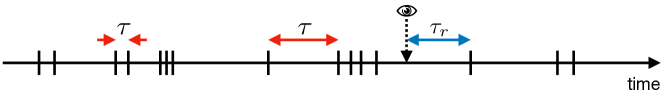
Note that there is another similar quantity, called the residual time (also called the residual waiting time), what we will use later during our discussion. It’s definition considers that the observations of an event sequence always cover a finite period and usually begins at a random moment of time. The time interval between the time of the observation and the first observed event is the residual time . Its distribution and average can be derived from the corresponding inter-event time distribution as
| (4) |
This result explains a phenomenon called the waiting-time paradox, which has important consequences in dynamical processes evolving on bursty temporal systems as will be discussed later.
The burstiness parameter
The heterogeneity of the inter-event times can be quantified by a single measure introduced by Goh and Barabási [goh2008burstiness]. The burstiness parameter is defined as the function of the coefficient of variation (CV) of inter-event times to measures temporal heterogeneity as follows:
| (5) |
Here takes the value of for regular time series with , and it is equal to for random, Poissonian time series where . In case when the time series appears with more heterogeneous inter-event times than a Poisson process, the burstiness parameter is positive (), while taking the value of only for extremely bursty cases with . Note that this measure has been recently shown to have some finite size effect, and an alternative measure has been introduced to account for these shortcomings [kim2016measuring].
The autocorrelation function
The conventional way for detecting correlations in time series is to measure the autocorrelation function. To define we use the representation of event sequences as binary signals and introduce the delay time , which sets a time lag between two observations of the signal . Then the autocorrelation function with delay time is defined as follows:
| (6) |
where denotes the time average over the observation period [box2008time]. In time series with temporal correlations, typically decays as a power law:
| (7) |
with decaying exponent . In addition, this measure can be related to the power spectrum or spectral density of the signal as follows:
| (8) |
which appears as the Fourier transform of autocorrelation function, indicating dominant event frequencies present in the signal.
A scaling relation between the inter-event time and the autocorrelation exponents has been studied both analytically and numerically [lowen1993fractal, allegrini2009spontaneous, vajna2013modelling]. It has been shown that they relate as
| (11) |
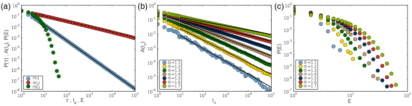
This indicates that the power-law decaying autocorrelation function could be explained solely by the inhomogeneous inter-event times and not by temporal correlations in the time series. In fact, the observed autocorrelation functions measure not only correlations between events but also between consecutive inter-event times of arbitrary length. Such correlations spuriously appear in independent heterogeneous time series disallowing autocorrelation to be a proper measure of real temporal correlations in bursty sequences. This is demonstrated in Fig. 3(a) where we built an independent event sequence by sampling randomly inter-event times from a power-law distribution with exponent (blue symbols) and measured the autocorrelation function in this uncorrelated signal. Due to the heterogeneity of the inter-event time distribution effective positive correlations are indicated by the autocorrelation, which emerges with a power-law tail (red symbols) even the sequence is independent. Fig. 3(b) demonstrates that the scaling exponent of the emerging autocorrelation function is dependent on the inter-event time distribution, in full agreement with the relation suggested in Eq. 11.
1 The Bursty Train Size Distribution
This ambiguity to detect short term temporal correlations in bursty event sequences motivated us to provide a new measure, which can decide evidently the presence of such dependencies, independently from the shape of the inter-event time distribution. More precisely, we made the qualitative observation that bursty events do not usually come in pairs but may form longer trains, where consecutive events may be in a causal relation with each other. However, to detect such bursty clusters in binary event sequence, , first we have to identify those events which we consider to be causally correlated. The smallest temporal scale at which correlations can emerge in the dynamics is between consecutive events. If only is known, we can assume two consecutive actions at and to be related if they follow each other within a short time interval, [wu2010evidence, turnbull2005string]. For events with the duration this condition is slightly modified: .
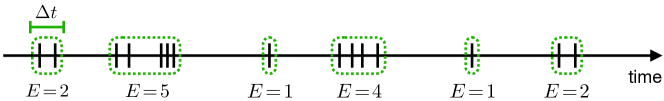
This definition allows us to detect bursty periods, defined as a sequence of events where each event follows the previous one within a time interval , as illustrated in Fig. 4. By counting the number of events, , that belong to the same bursty period, we can calculate their distribution . For a sequence of independent events, is uniquely determined by and the inter-event time distribution as follows:
| (12) |
for . Here the integral defines the probability to draw an inter-event time randomly from an arbitrary distribution , is a constant, and approximation appears due to the series expansion of the constant multiplicative term. The first term on the l.h.s. of Eq.12 gives the probability that we draw an inter-event times independently consecutive times, while the second term assigns that the drawing gives a therefore the evolving train size becomes exactly . If the measured time window is finite (), which is always the case here, the integral is a constant and the asymptotic behaviour appears like in a general exponential form. Consequently, for any finite independent event sequence the distribution decays exponentially even if the inter-event time distribution is fat-tailed. Deviations from this exponential behaviour indicate correlations in the timing of the consecutive events.
Bursty sequences in human communication
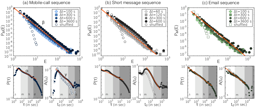
To check the scaling behaviour of in real systems we focused on outgoing events of individuals in three selected communication datasets: (a) A mobile-call dataset from a European operator (see DS1 in Section LABEL:sec:datasets); (b) Text message records from the same dataset (also DS1); and (c) Email communication sequences [eckmann2004entropy]. For each of these event sequences, the distribution of inter-event times measured between outgoing events are shown in Fig.5 (left bottom panels) and the estimated power-law exponent values are summarised in Table 1. The autocorrelation functions, which were averaged over randomly selected users with maximum time lag of , indicate strong temporal correlation (as seen in Fig.5.a and b (right bottom panels) with exponents in Table 1). The power-law behaviour in appears after a short period, denoting the reaction time through the corresponding channel, and lasts up to hours, capturing the natural rhythm of human activities. For emails in Fig.5.c (right bottom panels) long term correlation are detected up to hours, which reflects the typical length of office hours (note that the dataset includes internal email communication of a university staff).
| Mobile-call sequence | ||||
| Short message sequence | ||||
| Email sequence | ||||
| Model |
The broad shape of and functions confirm that human communication dynamics is heterogeneous and displays non-trivial correlations up to finite time-scales. However, after destroying event correlations by shuffling inter-event times in the interaction sequence of single individuals (see a how to in Section LABEL:sec:tnet_rrm) the autocorrelation function still shows slow power-law like decay (empty symbols on bottom right panels) via spurious residual dependencies. This clearly demonstrates the disability of to characterise correlations for heterogeneous signals, just as we have already seen for modelled signals. However as we have discussed earlier, the distribution should indicate evidently the presence of short temporal correlations. Calculating this distribution for various windows, we find that it depicts a scale invariant behaviour as
| (13) |
for each of the empirical event sequences as shown in the main panels of Fig.5. evidently indicates that there are strong temporal correlations in the empirical sequences as it is remarkably different from the corresponding distributions calculated for independent sequences which, as predicted by (12), appear with exponential decay (empty symbols on the main panels).
Exponential behaviour of was also expected from results published in the literature assuming human communication behaviour to be uncorrelated [malmgren2008poissonian, wu2010evidence, anteneodo2010poissonian]. However, the observed scaling behaviour of offers a direct evidence of correlations in human dynamics, which can arguably be responsible for the observed bursty dynamics. These correlations induce long bursty trains in the event sequence rather than short bursts of independent events. In addition, we have found that the scaling of the distribution is quite robust against the choice of for an extended regime of time-window sizes, or when it is computed for individuals or group people of similar activity level, or once the effects daily fluctuations are accounted for (for results see [karsai2011universal]).
Note that we observed long bursty event trains and similar scaling of their size in various natural phenomena, like in earthquake sequences recorded at given locations [smalley1987a, zhao2010non], or in the firing patterns of single neurons recorded in rat’s hypocampal. Corresponding results are not shown here but reported in [karsai2011universal].
3 Cyclic patterns in human dynamics
It is evident that humans follow intrinsic periodic patterns of circadian, weekly, and even longer cycles [malmgren2008poissonian, jo2012circadian, aledavood2015daily]. Such cycles clearly contribute to the inhomogeneities of temporal patterns, and they often result in an exponential cutoff to the inter-event time distributions. Identifying and filtering out such cyclic patterns from a time series can reveal bursty behaviour of different origins than those cycles [jo2012circadian]. In order to characterise such cyclic patterns, let us consider a time series, i.e., the number of events at time , denoted by , for the entire period of . One may be interested in a specific cycle, like daily or weekly ones, with period denoted by . Then, for a given period of , the event rate with can be defined as
| (14) |
Such cycles turn out to be also apparent in the inter-event time distributions . For example, one finds peaks of corresponding to multiples of one day in mobile phone communication as can be seen in Fig. 5a and b lower left panels. Note that such periodicities could be characterised by means of a power spectrum analysis in Eq. (8), however here we take another way.
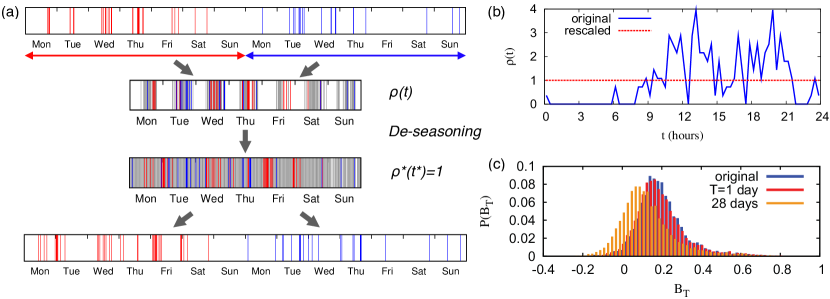
Once such cycles are identified in terms of the event rate , we can filter them by deseasoning the time series [jo2012circadian]. First, we extend indefinitely the domain of by with an arbitrary integer . Then using the identity of with the deseasoned event rate of , we can get the de-seasoned time as
| (15) |
For the schematic example of the de-seasoning method, see Fig. 6a. In plain words, the time is dilated (respectively contracted) at the moment of the high (respectively low) event rate resulting an overally constant average event rate as shown in as demonstrated in Fig. 6b. Then the de-seasoned event sequence of is compared to the original event sequence of to see how strong signature of burstiness or memory effects remained in the de-seasoned sequence. This reveals whether the empirically observed temporal heterogeneities can (or cannot) be explained by the intrinsic cyclic patterns, characterised in terms of the event rate. For example, one can measure the burstiness parameter for both the original and the de-seasoned mobile phone call series as shown in Fig. 6c using DS1 (see Section LABEL:sec:datasets). Although the distribution slightly changes after de-seasoning over a period , it assigns that the majority of individual sequences remain with positive bursty parameters.
One can also obtain the de-seasoned inter-event time corresponding to the original inter-event time as
| (16) |
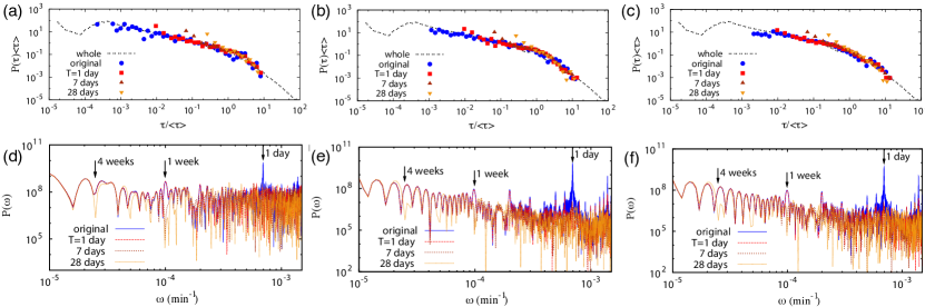
This way the de-seasoned inter-event time distribution can be compared to the original inter-event time distribution . As shown in Fig. 7a-c, the inter-event time distributions for the original and de-seasoned event sequences show almost the same shape for various values of and for individuals of various activity level. At the same time, it is evident from Fig. 7d-f, that after de-seasoning the circadian and weekly peaks of event frequencies disappear from the power spectra (for definition see Eq. 8), while its overall scaling remains very similar to the original spectrum. All these results together imply that bursty human dynamics cannot be exclusively explained by periodic circadian and weekly fluctuations, but it may have some other intrinsic behavioural origins.
I have another set of works [karsai2011small, kivela2012multiscale], which provide new tools to understand the effects and consequences of bursty interactions, through the introduction of random reference models of temporal networks. These works will be addressed in Section LABEL:sec:tnet_rrm as they provide tools to analyse temporal networks in general, not only bursty phenomena exclusively.
4 Observation of bursty phenomena
Bursty dynamics characterise human behaviour on the individual level and in turn may determine the evolution of dyadic interactions or the emergence of macroscopic phenomena in the social network. The dynamics of social networks can be discussed in terms of nodes, links, communities, or at the collective level, and can be characterised at different temporal scale, as we will discuss later in Chapter LABEL:ch:tnet on temporal networks. To address bursty dynamics of interactions, we distinguish between two temporal scales of link dynamics, which can be assigned to rather different types of behaviour. On one hand, we consider the slow dynamics of social link creation and decay, which determines the evolution of the social network. As an example, think about student mates with whom one may maintain a social relationship over years, which typically decay after graduation. On the other hand, we consider temporal interactions appearing with a rapid pace on existing social ties. These are for example calls, messages, or emails, which typically appear recurrently with high frequency and short duration as compared to the lifetime of a social tie. Next, I summarise some observational results we obtained on real social networks, published in [kikas2013bursty, karsai2012correlated], to see whether bursty characters appear in the interaction dynamics at these two temporal scales, and if yes, how these bursty interactions are distributed in the egocentric network of an individual.
1 Bursty egocentric network evolution
First let’s concentrate on the evolution of egocentric networks by analysing creation and decay of confirmed contacts in the online social-communication system of Skype [kikas2013bursty]. As we have already explained in Section LABEL:sec:datasets, the DS4 dataset contains the time stamps of approval of each Skype contacts (which can be regarded as times of link creation), and deletion of Skype contacts if it happened before the end of the observation period. In addition, we consider time series indicating the number of days in each month when the user connected to the Skype network, and also the adoption time (first usage) of each free service [e.g. Skype-to-Skype (S2S) audio calls, video calls, chat, etc.] together with time series indicating the number of days in each month when the user used the given service.
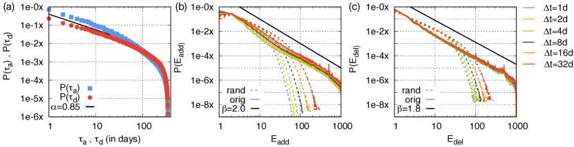
To characterise the temporal evolution of contact lists, we first examine the sequences of edge addition and deletion of each individual by calculating the distributions of inter-event times defined as (resp. ) between consecutive additions (resp. deletions) events of the same user. As demonstrated in Fig. 8a, these distributions are very heterogeneous both in case of edge additions and edge deletions. They show rather similar scaling, which can be approximated with a power-law function with exponent and an exponential cutoff. This is an interesting observation as one would expect rather different decision mechanisms behind adding and deleting a contact as additions can be assumed to be driven by the desire or need to communicate or to signal a social relation, while deletions are arguably driven by the desire not to be visible or accessible by the deleted contact.
To identify temporal correlations between consecutive actions of link additions or deletions, we locate bursty event trains and compute their size distributions using the methodology explained in Section 1. More precisely, we analysed the edge modification sequences of each individual and extracted the clusters of events of new edge addition and deletion (the trains) to record their size (resp. ). The fact that the (resp. ) distribution in Fig.8 spans over orders of magnitude, for several values, confirming the presence of correlations between consecutive events of edge additions (resp. deletions). This is even more apparent once we compare the empirical functions to the equivalent distributions calculated for independent sequences where inter-event times has been randomly shuffled. It puts into evidence that the actions of an individual are not independent and that the evolution of egocentric networks is not only heterogeneous in time but driven by intrinsic correlations. They lead to the presence of high activity bursty periods, where a large number of edges are added or deleted, separated by long low activity intervals.
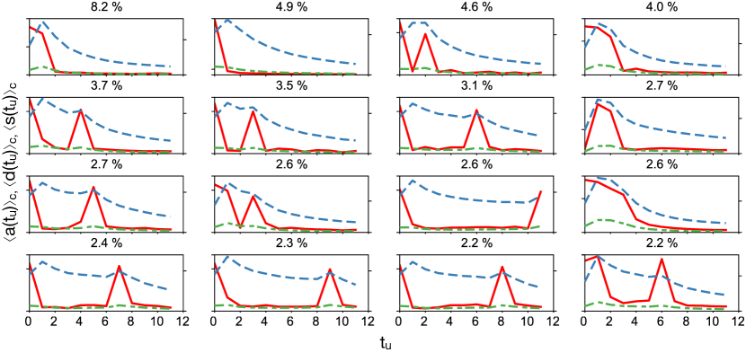
So far we have observed that edge addition and deletion events of an individual are bursty and clustered in time, yet we know less about when these bursty trains evolve during the lifetime of a user. Do they appear in any time or there are typical activity patterns of edge additions or maybe triggered by other user actions? To answer these questions, we compare the edge addition sequences of individuals during the first year of their user time after their registration [kikas2013bursty]. We keep track the number of newly added edges of each node in each month to obtain a discrete sequence for each individual with . To be able to compare sequences of users with diverse overall intensity we applied the Symbolic Aggregate Approximation (SAX) method [lin2003symbolic] with alphabet size 10, while to detect groups of users with similar edge addition dynamics, we applied the k-means clustering method on the activity sequences using euclidean distance. We determined the optimal cluster number to be by using the Elbow method. For the most populated clusters, the average link addition activity curves, , are shown in Fig. 9 (red line). Looking at the most common patterns it is straightforward that typically people perform their principal (the largest and usually the only one) edge addition burst right after they join the network, a behaviour which is confirmed by other studies [gaito2012bursty]. This is the time when they explore their social acquaintances who have already joined the system, while later they add contacts just occasionally with lower frequency. This behaviour and its significance has been demonstrated in [kikas2013bursty] (results not shown here). However, a single bursty peak at early time is not the characteristic of every user. Less common motifs in Fig.9 show that principal bursty peaks may emerge later or even in multiple times. This observation indicates that events other than user registration (e.g. adoption of different services) may also trigger immediate changes in the egocentric network. Actually, we found that the link addition dynamics is positively correlated (with coefficient ) with the overall activity of users (shown with blue lines in Fig.9), what we measured as the average number of connected days per month. Similarly, we found correlations with the activity of free service usage (with coefficient ), shown as green lines. More importantly, we showed that the probability of a user performing a link addition burst is strongly conditional to the adoption of free and payed services, which explains the emergent later peaks in the link addition dynamics (for further results see [kikas2013bursty]).
2 Bursty communication in egocentric networks
In our second empirical study let’s move from the level of social tie evolution to the level of time varying interactions in egocentric networks. Analysing interaction dynamics at this finer temporal scale, at which social ties are actually maintained, is a key to the better understanding of the evolution of egocentric networks and the emergent structural correlations in the social network (as we will discuss in Chapter LABEL:ch:tnet). As a demonstration, Fig. 10a illustrates mobile phone call patterns in an egocentric network, where the overall activity of the ego (green row) and activities on separated edges with three friends (orange rows) are presented. By looking at this picture we can draw three important observations: (a) the communication dynamics of the central ego (green) is evidently bursty with heterogeneous inter-event times and broad distribution (see Fig. 10d) with exponent (for SMS see [karsai2012correlated]); (b) The amount of communication efforts is not evenly distributed among ties (orange), but some ties carry the wast majority of interactions, while others are maintained by only a few events. It assigns differences in terms of social tie strengths, arguably associated to various level of intimacy as suggested by Dunbar [barrett2002human], and leads to heterogeneous link weight distributions on the network level; Finally, (c) correlated events form trains in bursty periods. The distribution of trains in the egocentric network can be explained by two competing hypothesises. On one hand, correlated event trains of the ego may evolve on single links (as seen on the zoom shown on panel Fig. 10b), which suggests that bursty periods are actually induced by dyadic interactions. On the other hand, as demonstrated in Fig. 10c, bursty communication periods of an ego may involve multiple peers, suggesting that bursty patterns are potentially induced by collective behaviour, the effort of a group e.g. to organise an event or to process information. As next [karsai2012correlated], our aim will be to empirically decide between these hypothesises by analysing DS1 mobile phone call and SMS datasets with the previously introduced characteristic methods of bursty phenomena.

More precisely, we are going to use the bursty train size distribution to indicate how trains are distributed in the egocentric topology. At first, let’s concentrate on ego-initiated events of outgoing voice calls and SMS’. In case we consider entire event sequences of egos, which combines all of their communications on any links, the distributions (shown for calls in Fig. 10b with solid lines) appear approximately as a power-law function with exponent (for SMS not shown [karsai2012correlated]). This behaviour is remarkably different from the scaling of the corresponding reference distributions, where inter-event times were randomly shuffled over the whole data (see exponential distributions with solid lines in Fig. 10b for calls). Based on this node centric view, intuitively one would assume that correlated outgoing communications of an individual may serve the information processing or organisation of a group [licoppe2005social, engestrom1999center], resulting events grouped in trains directed towards several neighbours. Assuming this mechanism to be dominant, burstiness would appear as the property of a single node or a group of individuals.
Surprisingly, the generic picture seems to be very different. If we assume that the correlated events in trains are directed toward several neighbours, decoupling event trains on single edges should induce an entirely different, less correlated statistics of bursts. However, this is not the case. The distributions, detected on single edges (shown for calls in Fig. 10b with dashed lines), are scaling very similarly and can be characterised by the same exponents as in the node centric case. This suggests that trains of events usually evolve on single links rather among a larger group of individuals. This picture is also supported by the statistics of temporal motifs [kovanen2011temporal], where motifs involving two individuals are by far the most common ones. The same conclusion can be drawn by counting the number of neighbours , whom an individual called in a bursty train of events. If a user communicates with only one neighbour during a period then the ratio , or if each call are directed toward different neighbours than . The distributions of the ratios for each train size (shown in Fig. 10e for calls, for SMS not shown [karsai2012correlated]) indicates that on average only one or two people are called in a bursty train independent of its size.
Next let’s have a look at the direction of event trains. Are they balanced or contain events dominantly initiated by one partner? Do voice calls and SMS’ are different from this point of view? First, let’s calculate the overall communication balance over the entire observation period for each edge as , where () are the total number of calls from to ( to ). Hence can vary between (completely balanced) and (completely imbalanced, dominated by one of the participants). We use this measure to compute the weighted average communication balance of trains on single edges with size evolving as:
| (17) |
where is the number of trains of length on edge . For SMS (brown squares in Fig.10.f) is converging to for larger sizes thus longer trains are more and more balanced in this case. This can be explained by the uni-directed information flow in case of SMS forcing mutual discussions to be more balanced, as it has been also argued by Wu et al. [wu2010evidence]. However, this constrain does not apply for the mobile calls (orange points in Fig.10.f) where information can flow in both directions during a call. Here reflects strongly unbalanced communication as it increases towards for trains with larger .
However, the average overall balance does not reflect evidently the communication balance evolving in single trains. Hence we define the communication balance within a train on an edge as . Here is the balance of the th train of length on edge connecting and , and () denotes the number of events initiated by (resp. ) towards (resp. ) in that train; . Averaging over trains of the same size gives an estimate for the average communication balance in trains of size (note that in this case different values can evolve even for trains on the same edge ). This has to be compared to the reference case, where trains of a given size follow the overall balance of the actual link. This can be calculated as
| (18) |
where the first term after the summation weights the binomial distribution taking into account that the imbalance can evolve in both directions, i.e., parallel or antiparallel to the imbalance of the edge. As depends only on and , the average can be taken as to get a reference estimate of and independent process.
Fig. 10.g shows and for both voice calls and SMS messages. Interestingly, large difference is observed between and the corresponding measures. It suggests that call trains (red points) are more unbalanced than one would expect from the overall communication balance of the link, caputured by the independent processes (yellow circles). At the same time for SMS the contrary is true as trains (blue squares) are much more balanced than one would derive from independent processes (green squares) reflecting the balance of the corresponding edges. This demonstrates real correlations between events of the same train and suggests different correlated mechanisms behind call and SMS dynamics.
5 Models of bursty human phenomena
As we have already explained in the introduction of this Chapter (Section 1), there are three main modelling frameworks, which have been proposed to explain the origin of bursty patterns in human dynamics. One framework provides a variety of models using priority queues [barabasi2005origin, oliveira2005human, vazquez2006modeling]; a second one is based on the assumption that consecutive actions of individuals are independent and can be modelled by Poisson processes with alternating time scales [malmgren2008poissonian, malmgren2009universality]; while the third direction assumes strong local correlations modelled by memory processes [vazquez2006impact, han2008modeling], self-excited point processes [masuda2013selfexciting, jo2015correlated], or reinforcement mechanisms [karsai2012correlated, wang2014modeling], etc. In the following, we are going to discuss two models [karsai2012correlated, karsai2011universal], proposed by me and colleagues, which belongs to the third modelling framework and employs reinforcement processes to model simultaneously temporal heterogeneities, bursty trains, or communication balance. While these models aim to explain phenomena observed on the individual or dyadic level, later in Section LABEL:sec:tnet_rrm we will discuss other models [karsai2011small, kivela2012multiscale], which address the emergence and effects of bursty phenomena on the collective level.
1 Model of individual bursty dynamics with event trains
According to the Decision Field Theory of psychology [busemeyer1993decision], each decision to perform a task can be interpreted as a threshold phenomenon, as the stimulus of the task has to reach a given threshold level to be chosen from the enormously large number of possible actions. This theory lays behind one possible interpretation of bursty behaviour, where the dynamics of an individual performing events of one certain task, like writing emails or printing, goes through active and inactive periods. An active state is initiated once the importance of the actual task overreach a certain level, which after the person performs a bursty cascade of events, while otherwise doing something else which in turn appears as long inactive periods in the actual observation. However, in active periods events are not independent from each other but form long bursty trains as we have already demonstrated in Section 1. Such dynamics can be explained by memory driven processes and modelled by reinforcement mechanisms as we explain next [karsai2011universal].
Memory process
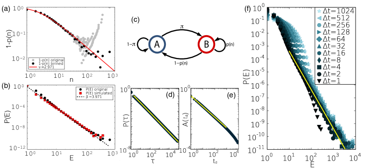
The correlations taking place between consecutive bursty events can be interpreted as a memory process, allowing us to calculate the probability that the individual will perform one more event within a time frame after it executed events previously in the actual train. This probability can be written as , thus its functional form is entirely coded in the train size distribution. If we assume that the actual train size distribution scales as (as already discussed in Eq.13) the memory function appears as
| (19) |
scaling relation is expect to hold as derived in [karsai2011universal]. To demonstrate that Eq. 19 holds for real systems, we measured the distribution for mobile calls in with seconds and derived the corresponding function. In Fig.11.a we show the complement of the empirical memory function, with strong finite size effects (grey dots) and the same function after logarithmic binning (black dots) on which we fit the theoretical memory function defined in Eq 19 using a non-linear least-squares method with only one free parameter, . As seen in Fig.11.a, we find that the best fit (red line) offers an excellent agreement with the empirical data with . Using the above mentioned exponent relation, this way we can estimate , which is close to the empirical value already reported in Table 1 and Fig 5a. To validate this approximation we generated bursty trains of events by using the theoretical memory function (defined in Eq. 19) with exponent and compared the scaling of the generated distribution to the corresponding empirical result. Results in Fig.11.b evidently demonstrate a good match between the simulated and empirical results, thus in turn they validate the chosen analytical form for the memory function (for more results see [karsai2011universal]).
Reinforcement model of bursty dynamics
Based on the above observations, we assume that the activity of an individual performing a task can be described with a two-state model, where a person can be in a normal state , executing independent events with longer inter-event times, or in an excited (bursty) state , performing correlated events with higher frequency. In this model we assume that inter-event times are determined by a reinforcement process, which dictates that the longer the system waits after an event, the larger the probability that it will keep waiting [stehle2010dynamical, zhao2011social]. Thus our two-state model is strongly non-Markovian as the timing of its events depends on the current and past states of the system. More precisely, given that our model system performed its last event time ago, the probability that it will wait one time unit longer without performing the next event is given as
| (20) |
where and control the reinforcement dynamics and the characteristic inter-event times in state and , respectively.
Finally, the model is defined as follows (for schematic demonstration see Fig.11.c, while an algorithmic description see Alg. 1): first the system performs an event in a randomly chosen initial state (line 2 in Alg. 1). If the last event was in the normal state , it waits for a time induced by (line 7), after which it switches to state with probability and performs an excited event (line 9 and 10); or with probability stays in the normal state and executes a new normal event. In the excited state the inter-event time for the actual event comes from after which the system executes one more excited event with a probability (see Eq. 19 and line 14 in Alg. 1) that depends on the number of excited events since the last normal event; otherwise it switches back to a normal state with probability (line 16).
[h!] Algorithmic description of the reinforcement model of bursty activity trains. {algorithmic}[1] \Statex\FunctionBursty reinforcement model \State \State \State \While \If \State \If \State \State \EndIf\State \ElsIf \State \If \State \Else\State \EndIf\State \EndIf\EndWhile\EndFunction
The results of the simulated model process, summarised in Fig. 11 and Table 1, indicates that the emergent inter-event time distribution appears with strong inhomogeneities (see Fig.11.d). It can be approximated by a scale-free function with exponent , which satisfies the expected exponent relation , similar to the one derived in Eq. 19. Beyond temporal heterogeneities we detect emergent long temporal correlations reflected by the power-law tail of the autocorrelation function (see Fig.11.e). It can be characterised by an exponent , which also satisfies the relation (as discussed in Section 2 and [karsai2011universal, vajna2013modelling]). Finally, the distribution appears with a fat-tail for each investigated window size ranging from to (see Fig.11.f), which can be characterised with an exponent in agreement with the expected relation in (Eq. 19). Note that the weak dependency of the simulated can be explained by the merge of correlated long bursty trains and uncorrelated single events which is more common for larger . Finally, once we fix the value of and , the emergent exponent satisfies the inequality , observed in empirical data (see Table 1).
2 Model of communication balance of dyadic event trains
In an extended model definition, introduced in [karsai2012correlated], we further used the memory function (in Eq. 19) to model the observed cases of communication balance in call and SMS sequences as reported in Section 2. To introduce this new model let us first concentrate on voice calls. One correlation we observed in Fig. 10.f was that longer event trains tend to be more unbalanced, meaning that they are more dominated by events initiated by one of the callers. Keeping in mind that mobile calls enable bidirectional information change, we assume that the observed unbalanced communication in interaction trains reflects the difference in motivation between the communicating partners. If there is a task to solve, which is more important for one party, it gives motivation for him/her to repeate calls until the issue gets settled. This mechanisms can be incorporated into the reinforcement process demonstrated in Fig.12.a, and can be summarised in the following way (note that its algorithmic solution is somewhat similar to Alg. 1 thus we do not present it here): We simulate bursty trains, which evolve on a link between a pair of individuals and . To initiate a train with a probability equal to we randomly select or who then perform one event towards the other agent and we set the actual train size to . The decision about the next event is carried out in two steps. First we decide with the probability in Eq.19 whether to perform one more event in the train or initiate a new train otherwise. If the train should be continued the probabilities that the next event is initiated by or are
| (21) |
where . Here denotes the probability that the th event of the actual train is performed by the same user who initiated the train at , while is the probability that the other agent initiates the event. Consequently, the longer a train evolves, the larger is the probability that the agent, who initiated the actual train, will initiate the next event. Eq.19 and Eq.21 may capture the entangled mechanisms of reinforced motivation of an individual, which is induced by the effort already invested in the actual series of calls to successfully solve a task with the other partner.
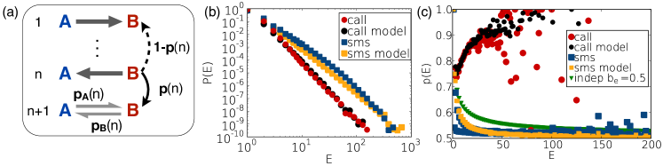
In case of SMS sequences the mechanism for developing strong balance in bursty trains is different. There, in single events information can pass only one way and consecutive events in a train usually have reversed direction, possibly forming strongly balanced conversations. To simulate this behaviour we use the above defined generative process but we select the direction of the actual event differently. Here we assume that the direction of an event conditioned only on the orientation of the previous event, and can be determined by the conditional probabilities
| (22) |
where and denotes the probability to choose the opposite direction for the th event compared to the one in the th step. Accordingly denotes the probability of choosing the same direction as the previous event. This way, the longer a train evolves, the larger is the probability to revert the direction of consecutive events and consequently to generate more balanced train.
The emergence of enhanced balance/imbalance in trains can be evidently checked on links where the overall communication is completely balanced and the communication balance of trains comes only from actual behavioural differences. To do so we set and compare the modelled results to averages calculated for similar empirical trains. To analyse real trains we select edges from the mobile call network with overall balance (there are calls and SMS on such links) and after detecting trains we calculate the corresponding distribution and function (defined in Section 2). As expected and shown in Fig.12.b, the size of call trains (red circles) detected with and SMS trains (blue squares) with are distributed broadly with characteristic exponents and , accordingly. Using these exponents as parameters we modelled event sequences to simulate calls and SMS trains with the same number of events and corresponding exponents deduced from according to Eq.19. The size distributions of model call trains (black circles) and model SMS trains (yellow squares) collapse surprisingly well on the corresponding empirical functions, as shown in Fig.12.b.
At the same time, in Fig. 12.c the balance functions calculated for the limited event sets on fully balanced links show surprisingly similar behaviour to the overall averages (seen in Fig. 10.g). This demonstrates that even an overall balanced link, strong communication imbalances appear due to local correlations within one bursty train. This is even more striking if we compare the empirical P(E) curves to the corresponding independent one (green triangles in Fig.12.c) which was generated using Eq.18 with . Moreover, in Fig. 12, the average balance functions emerging without parameters for model trains are in surprisingly good agreement with the empirical observations. Consequently, the assumed mechanisms defined in Eq. 21 and 22 are capturing rather accurately the salient features of the dynamics of directed human communication through phone calls and SMS. The only discrepancy is for the values of short SMS trains, where the empirical data show an even-odd effect, which is not reproduced in the model. This indicates that possibly other mechanism may be present in the communication sequence what are not considered in this modelling study.
6 Conclusions
In this Chapter, I summarised my most important results in one of my main research domains on bursty human dynamics. After a brief overview of the field, first I introduced some basic characteristic measures, some of them defined by me and colleagues, which are commonly used to quantify heterogeneous patterns in human dynamics. Subsequently, I systematically walked through a series of studies I published over the last years for the advanced characterisation, observation, and modelling of bursty human dynamics.
Due to the diverse experiences, broad overview, and devoted interest towards this field, together with Dr. Hang-Hyun Jo and Pr. Kimmo Kaski, we recently took the timely opportunity to write a monograph book, entitled as ”Bursty Human Dynamics“, to review all relevant knowledge on the field cumulated over the last decade. This book has been published by Springer in January 2018.
Finally note that some of my studies published on the system-level observations, modelling, and effects of bursty dynamical patterns are not mentioned in this Chapter as they land close to field of temporal networks, which is the topic of the coming Chapter.