Entropy Symmetrization and High-Order Accurate Entropy Stable Numerical Schemes for Relativistic MHD Equations

Abstract

This paper presents entropy symmetrization and high-order accurate entropy stable schemes for the relativistic magnetohydrodynamic (RMHD) equations. It is shown that the conservative RMHD equations are not symmetrizable and do not admit a thermodynamic entropy pair. To address this issue, a symmetrizable RMHD system, equipped with a convex thermodynamic entropy pair, is first proposed by adding a source term into the equations, providing an analogue to the non-relativistic Godunov–Powell system. Arbitrarily high-order accurate entropy stable finite difference schemes are developed on Cartesian meshes based on the symmetrizable RMHD system. The crucial ingredients of these schemes include (i) affordable explicit entropy conservative fluxes which are technically derived through carefully selected parameter variables, (ii) a special high-order discretization of the source term in the symmetrizable RMHD system, and (iii) suitable high-order dissipative operators based on essentially non-oscillatory reconstruction to ensure the entropy stability. Several numerical tests demonstrate the accuracy and robustness of the proposed entropy stable schemes.

35L65, 65M12, 65M06, 76W05, 76Y05

1 Introduction

Magnetohydrodynamics (MHDs) describe the dynamics of electrically-conducting fluids in the presence of magnetic field and play an important role in many fields including astrophysics, plasma physics and space physics. In many cases, astrophysics and high energy physics often involve fluid flow at nearly speed of light so that the relativistic effect should be taken into account. Relativistic MHDs (RMHDs) have applications in investigating astrophysical scenarios from stellar to galactic scales, e.g., gamma-ray bursts, astrophysical jets, core collapse super-novae, formation of black holes, and merging of compact binaries.

In the $d$-dimensional space, the governing equations of special RMHDs can be written as a system of hyperbolic conservation laws

(1) $$\frac{{\partial{\bf U}}}{{\partial t}}+\sum_{i=1}^{d}\frac{\partial{\bf F}_{i}({\bf U})}{\partial x_{i}}={\bf 0},$$

along with an additional divergence-free condition on the magnetic field

(2) $$\nabla\cdot{\bf B}:=\sum_{i=1}^{d}\frac{\partial B_{i}}{\partial x_{i}}=0,$$

where $d=1,$ $2$ or $3$. Here we employ the geometrized unit system so that the speed of light $c$ in vacuum is equal to one. In (1), the conservative vector ${\bf U}=(D,{\bf m}^{\top},{\bf B}^{\top},E)^{\top}$, and the flux in the $x_{i}$-direction is defined by

$${\bf F}_{i}({\bf U})=\left(Dv_{i},v_{i}{\bf m}^{\top}-B_{i}\big{(}\gamma^{-2}{\bf B}^{\top}+({\bf v}\cdot{\bf B}){\bf v}^{\top}\big{)}+p_{tot}{\bf e}_{i}^{\top},v_{i}{\bf B}^{\top}-B_{i}{\bf v}^{\top},m_{i}\right)^{\top},$$

with the mass density $D=\rho\gamma$, the momentum density vector ${\bf m}=(\rho h{\gamma^{2}}+|{\bf B}|^{2}){\bf v}-({\bf v}\cdot{\bf B}){\bf B}$, the energy density $E=\rho h\gamma^{2}-p_{tot}+|{\bf B}|^{2}$, and the vector ${\bf e}_{i}$ denoting the $i$-th column of the unit matrix of size $3$. Additionally, $\rho$ is the rest-mass density, ${\bf v}=(v_{1},v_{2},v_{3})^{\top}$ denotes the fluid velocity vector, $\gamma=1/\sqrt{1-|{\bf v}|^{2}}$ is the Lorentz factor, $p_{tot}$ is the total pressure containing the gas pressure $p$ and magnetic pressure $p_{m}:=\frac{1}{2}\left(\gamma^{-2}|{\bf B}|^{2}+({\bf v}\cdot{\bf B})^{2}\right)$, $h=1+e+\frac{p}{\rho}$ represents the specific enthalpy, and $e$ is the specific internal energy. We consider the ideal equation of state $p=(\Gamma-1)\rho e$ to close the system (1), where $\Gamma$ is constant and denotes the adiabatic index.

The system (1) involves strong nonlinearity, making its analytic treatment quite difficult. Numerical simulation is a primary approach to explore physical laws in RMHDs. The numerical study of RMHDs may date back to the 1990s, to the best of our knowledge. For instance, the time-dependent morphological evolution of a RMHD jet was computed in [61], based on a divergence-free formation of the Maxwell equations coupled to fluids [59] with the numerical method proposed in [60]. During the past few decades, various numerical schemes have been developed for the RMHD equations, including but not limited to: the total variation diminishing scheme [3], adaptive mesh methods [58, 35], discontinuous Galerkin methods [67, 68], physical-constraints-preserving schemes [66], entropy limited approach [32], etc. Systematic review of numerical RMHD schemes is beyond the scope of the present paper, and we refer interested readers to the review articles [26, 44]. Besides the standard difficulty in solving the nonlinear hyperbolic systems, an additional numerical challenge for the RMHD system (1) comes from the divergence-free condition (2), which is also involved in the non-relativistic ideal MHD system. Numerical preservation of (2) is highly non-trivial (for $d\geq 2$) but crucial for the robustness of numerical computations. Numerical experiments and analysis in the non-relativistic MHD case indicated that violating the divergence-free condition (2) may lead to numerical instability and nonphysical solutions [9, 4, 63]. Various numerical techniques were proposed to reduce or control the effect of divergence error; see, e.g., [20, 50, 56, 16, 4, 41, 42, 64, 65].

Due to the nonlinear hyperbolic nature of the RMHD equations (1), solutions of (1) can be discontinuous with the presence of shocks or contact discontinuities. This leads to the consideration of weak solutions. However, weak solutions may not be unique. To select the “physically relevant” solution among all weak solutions, entropy conditions are usually imposed as the admissibility criterion. In the case of RMHD equations (1), there is a natural entropy condition arising from the second law of thermodynamics which should be respected. It is natural to seek entropy stable numerical schemes which satisfy a discrete version of that entropy condition. Entropy stable numerical methods ensure that the entropy is conserved in smooth regions and dissipated across discontinuities. Thus, the numerics precisely follow the physics of the second law of thermodynamics and can be more robust. Moreover, entropy stable schemes also allow one to limit the amount of dissipation added to the schemes to guarantee the entropy stability. For the above reasons, developing entropy stable schemes for RMHD equations (1) is meaningful and highly desirable.

Entropy stability analysis was well studied for first-order accurate schemes and scalar conservation laws [14, 34, 47, 48]. For systems of hyperbolic conservation laws, much attention was paid to explore entropy stable schemes with entropy stability focused on single given entropy function. Tadmor [53, 54] established the framework of entropy conservative fluxes, which conserves entropy locally, and entropy stable fluxes for second-order schemes. Lefloch, Mercier and Rohde [40] proposed a procedure to construct higher-order accurate entropy conservative fluxes. Fjordholm, Mishra and Tadmor [23] developed a methodology for constructing high-order accurate entropy stable schemes, which combine high-order entropy conservative fluxes and suitable numerical dissipation operators based on essentially non-oscillatory (ENO) reconstruction that satisfies the sign property [24]. On the other hand, high-order entropy stable schemes have also been constructed via the summation-by-parts (SBP) procedure [21, 10, 28]. Entropy stable space–time discontinuous Galerkin (DG) schemes were studied in [5, 6, 37], where the exact integration is required for the proof of entropy stability. More recently, a framework for designing entropy stable high-order DG methods through suitable numerical quadrature was proposed in [13], where the SBP operators established in [21, 10, 28] were used and also generalized to triangles. There are other studies that address various aspects of entropy stability, including but not limited to [8, 25, 7, 36]. As a key ingredient in designing entropy stable schemes, the construction of affordable entropy conservative fluxes has received much attention. Although there is a general way to construct entropy conservative fluxes based on path integration [53, 54], the resulting fluxes may not have an explicit formula and can be computationally expensive. Explicit entropy conservative fluxes were derived for the Euler equations [38, 11, 51], shallow water equations [29], special relativistic hydrodynamics without magnetic field [19], and ideal non-relativistic MHD equations [12, 62], etc. Different from the Euler equations, the conservative non-relativistic MHD equations are not symmetrizable and do not admit an entropy [31, 5, 12]. Entropy symmetrization can be achieved by a modified system with an additional source [31, 5]. Based on the modified formulation, several entropy stable schemes were developed for non-relativistic MHDs; see, e.g., [12, 17, 62, 43, 18].

This paper aims to present entropy analysis and high-order accurate entropy stable schemes for the RMHD equations on Cartesian meshes. The difficulties in this work mainly come from the highly nonlinear coupling between RMHD equations (1), which leads to no explicit expression of the primitive variables $(\rho,{\bf v},p)$, entropy variables and fluxes ${\bf F}_{i}$ in terms of ${\bf U}$. The effort and findings in this work include the following:

1. We show that the conservative form (1) of RMHD equations is not symmetrizable and thus does not admit a thermodynamic entropy pair. A modified RMHD system is proposed by building the divergence-free condition (2) into the equations through adding a source term, which is proportional to $\nabla\cdot{\bf B}$. The modified RMHD system is symmetrizable, possesses a convex thermodynamic entropy pair, and is an analogue to the non-relativistic symmetrizable MHD system proposed by Godunov [31] and Powell [50]. The Godunov-type entropy symmetrization procedure was also briefly described in [57] and was first performed in [52] for RMHDs.

2. We derive a consistent two-point entropy conservative numerical flux for the symmetrizable RMHD equations. The flux has an explicit analytical formula, is easy to compute and thus is affordable. The key is to carefully select a set of parameter variables which can explicitly express the entropy variables and potential fluxes in simple form. Due to the presence of the source term in the symmetrizable RMHD system, the standard framework [54] of the entropy conservative flux is not applicable here and should be modified to take the effect of the source term into account.

3. We construct semi-discrete high-order accurate entropy conservative schemes and entropy stable schemes for symmetrizable RMHD equations on Cartesian meshes. The second-order entropy conservative schemes are built on the proposed two-point entropy conservative flux and a central difference discretization to the source term. Higher-order entropy conservative schemes are constructed by suitable linear combinations [40] of the proposed two-point entropy conservative flux. To ensure the entropy conservative property and high-order accuracy, a suitable discretization of the symmetrization source term should be employed, which is a key ingredient in these high-order schemes. Arbitrarily high-order accurate entropy stable schemes are obtained by adding suitable dissipation terms into the entropy conservative schemes.

It is noticed that high-order accurate entropy stable schemes were developed in a very recent work [19] for the relativistic hydrodynamics (RHDs) without the magnetic field, whose governing equations are sometimes also called the relativistic Euler equations. To the best of our knowledge, the present paper is the first to study entropy stable schemes for the RMHD equations. Note that, in the RMHD system, the magnetic field, evolved by the induction equations, is also nonlinearly involved in the momentum and energy equations. Due to the presence of magnetic field, mathematical structures of the RMHD system are more complicated than the relativistic Euler system, making the present derivations of entropy stable schemes more difficult. Different from the relativistic Euler equations whose conservative form admits a thermodynamic entropy pair [19], the conservative form (1) of the RMHD system does not admit the thermodynamic entropy pair, so that entropy symmetrization of the RMHD system must be derived to accommodate an entropy condition on the PDE level. Moreover, the symmetrization source term added in the modified RMHD system also renders additional technical challenges on the numerical level, since a suitable high-order discretization of that source term must be devised such that the resulting numerical schemes satisfy entropy stability. These make the exploration in this work significantly different from those in [19] and highly nontrivial. When the magnetic field is zero, the proposed entropy stable schemes for the RMHDs reduce to a class of entropy stable schemes for the RHDs. It is also worth mentioning that our entropy conservative fluxes are derived through a set of carefully selected parameter variables, which are different from those used in [19] for the RHDs, rendering the expression of our resulting fluxes simpler; see Remark 3.4 for details.

The paper is organized as follows. After giving the entropy analysis in Sect. 2, we derive the explicit two-point entropy conservative fluxes in Sect. 3. One-dimensional (1D) entropy conservative schemes and entropy stable schemes are constructed in Sect. 4, and their extensions to two dimensions (2D) are presented in Sect. 5. We conduct numerical tests in Sect. 6 to verify the performance of the proposed high-order accurate entropy stable schemes, before concluding the paper in Sect. 7.

2 Entropy Analysis

First, let us recall the definition of an entropy function.

Definition 2.1.

A convex function ${\mathcal{E}}({\bf U})$ is called an entropy for the system (1) if there exist entropy fluxes ${\mathcal{Q}}_{i}({\bf U})$ such that

(3) $${\mathcal{Q}}^{\prime}_{i}({\bf U})={\mathcal{E}}^{\prime}({\bf U}){\bf F}^{\prime}_{i}({\bf U}),\qquad i=1,\dots,d,$$

where the gradients ${\mathcal{E}}^{\prime}({\bf U})$ and ${\mathcal{Q}}^{\prime}_{i}({\bf U})$ are written as row vectors, and ${\bf F}^{\prime}_{i}({\bf U})$ is the Jacobian matrix. The functions $({\mathcal{E}},{\mathcal{Q}}_{i})$ form an entropy pair.

If a hyperbolic system of conservation laws admits an entropy pair, then the smooth solutions of the system should satisfy

$$0={\mathcal{E}}^{\prime}({\bf U})\left(\frac{{\partial{\bf U}}}{{\partial t}}+\sum_{i=1}^{d}\frac{\partial{\bf F}_{i}({\bf U})}{\partial x_{i}}\right)={\mathcal{E}}^{\prime}({\bf U})\frac{{\partial{\bf U}}}{{\partial t}}+\sum_{i=1}^{d}{\mathcal{Q}}^{\prime}_{i}({\bf U})\frac{\partial{\bf U}}{\partial x_{i}}=\frac{\partial{\mathcal{E}}}{\partial t}+\sum_{i=1}^{d}\frac{\partial{\mathcal{Q}}_{i}}{\partial x_{i}}.$$

Solutions of a nonlinear hyperbolic system can be discontinuous. This leads to the consideration of weak solutions, which, however, may not be unique, and for (non-smooth) weak solutions the above identity does not hold in general. The following inequality (see, e.g., [15, page 83]) is usually imposed as an admissibility criterion to select the “physically relevant” solution among all weak solutions:

(4) $$\frac{\partial{\mathcal{E}}}{\partial t}+\sum_{i=1}^{d}\frac{\partial{\mathcal{Q}}_{i}}{\partial x_{i}}\leq 0,$$

which is interpreted in the sense of distribution and known as an entropy condition.

The existence of an entropy pair is closely related to the symmetrization of a hyperbolic system of conservation laws [30].

Definition 2.2.

The system (1) is said to be symmetrizable if there exists a change of variables ${\bf U}\to{\bf W}$ which symmetrizes it, that is, the equations (1) become

(5) $$\frac{\partial{\bf U}}{\partial{\bf W}}\frac{\partial{\bf W}}{\partial t}+\sum_{i=1}^{d}\frac{\partial{\bf F}_{i}}{\partial{\bf W}}\frac{\partial{\bf W}}{\partial x_{i}}={\bf 0},$$

where the matrix $\frac{\partial{\bf U}}{\partial{\bf W}}$ is symmetric positive definite and $\frac{\partial{\bf F}_{i}}{\partial{\bf W}}$ is symmetric for all $i$.

Lemma 2.3.

A necessary and sufficient condition for the system (1) to possess a strictly convex entropy ${\mathcal{E}}({\bf U})$ is that there exists a change of dependent variables ${\bf U}\to{\bf W}$ which symmetrizes (1).

The proof of Lemma 2.3 can be found in [30].

2.1 Entropy Function for RMHD Equations

It is natural to ask whether the RMHD equations (1) admit an entropy pair or not.

Let us consider the thermodynamic entropy $S=\ln(p\rho^{-\Gamma}).$ For smooth solutions, the RMHD equations (1) can be used to derive an equation for $\rho\gamma S$:

(6) $$\frac{\partial(\rho\gamma S)}{\partial t}+\nabla\cdot(\rho\gamma S{\bf v})+(\Gamma-1)\frac{\rho\gamma({\bf v}\cdot{\bf B})}{p}\nabla\cdot{\bf B}=0.$$

Then under the divergence-free condition (2), the following quantities

(7) $${\mathcal{E}}({\bf U})=-\frac{\rho\gamma S}{\Gamma-1},\qquad{\mathcal{Q}}_{i}({\bf U})=-\frac{\rho\gamma Sv_{i}}{\Gamma-1}$$

satisfy an additional conservation law, thus ${\mathcal{E}}$ may be an entropy function.

Theorem 2.4.

The entropy variables corresponding to the entropy function ${\mathcal{E}}$ are

(8) $${\bf W}={\mathcal{E}}^{\prime}({\bf U})^{\top}=\left(\frac{\Gamma-S}{\Gamma-1}+\frac{\rho}{p},~{}\frac{\rho\gamma}{p}{\bf v}^{\top},~{}\frac{\rho\gamma}{p}\Big{(}(1-|{\bf v}|^{2}){\bf B}^{\top}+({\bf v}\cdot{\bf B}){\bf v}^{\top}\Big{)},~{}-\frac{\rho\gamma}{p}\right)^{\top}.$$

Proof 2.5.

Since ${\mathcal{E}}$ cannot be explicitly expressed by ${\bf U}$, direct derivation of ${\mathcal{E}}^{\prime}({\bf U})$ can be quite difficult. Here we consider the following primitive variables

(9) $${\bf V}=\left(\rho,{\bf v}^{\top},{\bf B}^{\top},p\right)^{\top}.$$

As ${\mathcal{E}}$ and $\bf U$ can be explicitly formulated in terms of ${\bf V}$, it is easy to derive that

$${\mathcal{E}}^{\prime}({\bf V})=\frac{1}{\Gamma-1}\left(\gamma(\Gamma-S),~{}-\rho S\gamma^{3}{\bf v}^{\top},~{}0,~{}0,~{}0,~{}-\frac{\rho\gamma}{p}\right),$$

(10) $$\frac{\partial{\bf U}}{\partial{\bf V}}=\begin{pmatrix}\gamma&\rho\gamma^{3}{\bf v}^{\top}&{\bf 0}_{3}^{\top}&0\\ \gamma^{2}{\bf v}&(\rho h\gamma^{2}+|{\bf B}|^{2}){\bf I}_{3}-{\bf B}{\bf B}^{\top}+2\rho h\gamma^{4}{\bf v}{\bf v}^{\top}&-({\bf v}\cdot{\bf B}){\bf I}_{3}+2{\bf v}{\bf B}^{\top}-{\bf B}{\bf v}^{\top}&\frac{\Gamma\gamma^{2}}{\Gamma-1}{\bf v}\\ {\bf 0}_{3}&{\bf O}_{3}&{\bf I}_{3}&{\bf 0}_{3}\\ \gamma^{2}&(2\rho h\gamma^{4}+|{\bf B}|^{2}){\bf v}^{\top}-({\bf v}\cdot{\bf B}){\bf B}^{\top}&(1+|{\bf v}|^{2}){\bf B}^{\top}-({\bf v}\cdot{\bf B}){\bf v}^{\top}&\frac{\Gamma\gamma^{2}}{\Gamma-1}-1\end{pmatrix},$$

where ${\bf 0}_{3}=(0,0,0)^{\top}$, and ${\bf O}_{3}$ and ${\bf I}_{3}$ denote the zero square matrix and the identity matrix of size $3$, respectively. One can verify that the vector $\bf W$ satisfies ${\bf W}^{\top}\frac{\partial{\bf U}}{\partial{\bf V}}={\mathcal{E}}^{\prime}({\bf V}),$ which implies ${\bf W}^{\top}={\mathcal{E}}^{\prime}({\bf V})\left(\frac{\partial{\bf U}}{\partial{\bf V}}\right)^{-1}={\mathcal{E}}^{\prime}({\bf V})\frac{\partial{\bf V}}{\partial{\bf U}}={\mathcal{E}}^{\prime}({\bf U}).$

However, the change of variable ${\bf U}\to{\bf W}$ fails to symmetrize the RMHD equations (1), and the functions $({\mathcal{E}},{\mathcal{Q}}_{i})$ defined in (7) do not form an entropy pair for the RMHD equations (1); see the following theorem.

Theorem 2.6.

For RMHD equations (1) and the entropy variables $\bf W$, one has

1. the change of variable ${\bf U}\to{\bf W}$ fails to symmetrize the RMHD equations (1), i.e., the matrix $\frac{\partial{\bf F}_{i}}{\partial{\bf W}}$ is not symmetric in general.

2. the functions $({\mathcal{E}},{\mathcal{Q}}_{i})$ defined in (7) satisfy

   (11) $${\mathcal{Q}}^{\prime}_{i}({\bf U})={\mathcal{E}}^{\prime}({\bf U}){\bf F}^{\prime}_{i}({\bf U})+\frac{\rho\gamma}{p}({\bf v}\cdot{\bf B})B_{i}^{\prime}({\bf U}),\quad i=1,\dots,d,$$

   which implies that $({\mathcal{E}},{\mathcal{Q}}_{i})$ do not satisfy the condition (3).

Proof 2.7.

We only prove the conclusions for $i=1$, as the proofs for $2\leq i\leq d$ are similar. Let us first show that $\frac{\partial{\bf F}_{i}}{\partial{\bf W}}$ is not symmetric in general. Because ${\bf F}_{1}$ cannot be formulated explicitly in terms of $\bf W$, we calculate the Jacobian matrix ${\bf F}_{1}({\bf W})$ with the aid of primitive variables ${\bf V}$. The Jacobian matrix $\frac{\partial{\bf F}_{1}}{\partial{\bf V}}$ is computed as

(12) $$\frac{\partial{\bf F}_{1}}{\partial{\bf V}}=v_{1}\frac{\partial{\bf U}}{\partial{\bf V}}+\begin{pmatrix}0&\rho\gamma{\bf e}_{1}^{\top}&{\bf 0}_{3}^{\top}&0\\ {\bf 0}_{3}&(\rho h\gamma^{2}+|{\bf B}|^{2}){\bf v}{\bf e}_{1}^{\top}+{\bf M}_{1}&{\bf M}_{2}&{\bf e}_{1}\\ {\bf 0}_{3}&{\bf B}{\bf e}_{1}^{\top}-B_{1}{\bf I}_{3}&-{\bf v}{\bf e}_{1}^{\top}&{\bf 0}_{3}\\ 0&(\rho h\gamma^{2}+|{\bf B}|^{2}){\bf e}_{1}^{\top}-B_{1}{\bf B}^{\top}+v_{1}\left(({\bf v}\cdot{\bf B}){\bf B}-|{\bf B}|^{2}{\bf v}\right)^{\top}&\bm{\beta}_{1}^{\top}-({\bf v}\cdot{\bf B}){\bf e}_{1}^{\top}&v_{1}\end{pmatrix},$$

with ${\bf e}_{1}=(1,0,0)^{\top}$, ${\bm{\beta}}_{1}=v_{1}(1-|{\bf v}|^{2}){\bf B}^{\top}+v_{1}({\bf v}\cdot{\bf B}){\bf v}^{\top}-B_{1}{\bf v}^{\top}$, and

$${\bf M}_{1}={\bf e}_{1}\big{(}({\bf v}\cdot{\bf B}){\bf B}^{\top}-|{\bf B}|^{2}{\bf v}^{\top}\big{)}+B_{1}(2{\bf B}{\bf v}^{\top}-{\bf v}{\bf B}^{\top})-({\bf v}\cdot{\bf B})(B_{1}{\bf I}_{3}+{\bf B}{\bf e}_{1}^{\top})$$

$${\bf M}_{2}=(1-|{\bf v}|^{2})({\bf e}_{1}{\bf B}^{\top}-{\bf B}{\bf e}_{1}^{\top})+({\bf v}\cdot{\bf B})({\bf e}_{1}{\bf v}^{\top}-{\bf v}{\bf e}_{1}^{\top})-B_{1}{\bf v}{\bf v}^{\top}-B_{1}(1-|{\bf v}|^{2}){\bf I}_{3}.$$

Since ${\bf W}$ can be explicitly expressed in terms of $\bf V$, one can derive that

(13) $$\frac{\partial{\bf W}}{\partial{\bf V}}=\begin{pmatrix}h/p&{\bf 0}_{3}^{\top}&{\bf 0}_{3}^{\top}&-\frac{\rho}{p^{2}}-\frac{1}{p(\Gamma-1)}\\ \frac{\gamma}{p}{\bf v}&\frac{\rho\gamma^{3}}{p}{\bf M}_{3}&{\bf O}_{3}&-\frac{\rho\gamma}{p^{2}}{\bf v}\\ \frac{\gamma}{p}((1-|{\bf v}|^{2}){\bf B}+({\bf v}\cdot{\bf B}){\bf v})&\frac{\rho\gamma^{3}}{p}{\bf M}_{4}&\frac{\rho\gamma}{p}{\bf M}_{3}&-\frac{\rho\gamma}{p^{2}}((1-|{\bf v}|^{2}){\bf B}+({\bf v}\cdot{\bf B}){\bf v})\\ -\frac{\gamma}{p}&-\frac{\rho\gamma^{3}}{p}{\bf v}^{\top}&{\bf 0}_{3}^{\top}&\frac{\rho\gamma}{p^{2}}\end{pmatrix},$$

with ${\bf M}_{3}=(1-|{\bf v}|^{2}){\bf I}_{3}+{\bf v}{\bf v}^{\top},{\bf M}_{4}=({\bf v}\cdot{\bf B}){\bf v}{\bf v}^{\top}+\gamma^{-2}\left[({\bf v}\cdot{\bf B}){\bf I}_{3}+{\bf v}{\bf B}^{\top}-{\bf B}{\bf v}^{\top}\right].$ Then, we obtain $\frac{\partial{\bf V}}{\partial{\bf W}}$ by the inverse of the matrix $\frac{\partial{\bf W}}{\partial{\bf V}}$, i.e.

(14) $$\frac{\partial{\bf V}}{\partial{\bf W}}=\begin{pmatrix}\rho&\left(\rho+\frac{p}{\Gamma-1}\right)\gamma{\bf v}^{\top}&{\bf 0}_{3}^{\top}&\left(\rho+\frac{p}{\Gamma-1}\right)\gamma\\ {\bf 0}_{3}&\frac{p}{\rho\gamma}{\bf I}_{3}&{\bf O}_{3}&\frac{p}{\rho\gamma}{\bf v}\\ {\bf 0}_{3}&\frac{p\gamma}{\rho}{\bf M}_{5}&\frac{p\gamma}{\rho}\left({\bf I}_{3}-{\bf v}{\bf v}^{\top}\right)&\frac{p\gamma}{\rho}\left((1+|{\bf v}|^{2}){\bf B}-2({\bf v}\cdot{\bf B}){\bf v}\right)\\ p&ph\gamma{\bf v}^{\top}&{\bf 0}_{3}^{\top}&ph\gamma\end{pmatrix},$$

with ${\bf M}_{5}=2{\bf B}{\bf v}^{\top}-({\bf v}\cdot{\bf B}){\bf I}_{3}-{\bf v}\left((1-|{\bf v}|^{2}){\bf B}^{\top}+({\bf v}\cdot{\bf B}){\bf v}^{\top}\right).$ By the chain rule $\frac{\partial{\bf F}_{1}}{\partial{\bf W}}=\frac{\partial{\bf F}_{1}}{\partial{\bf V}}\frac{\partial{\bf V}}{\partial{\bf W}}$, we get the expression of $\frac{\partial{\bf F}_{1}}{\partial{\bf W}}$ and find it is not symmetric in general. For example, the $(2,6)$ element of the Jacobian matrix $\frac{\partial{\bf F}_{1}}{\partial{\bf W}}$ is $\frac{p\gamma B_{2}}{\rho}(1+v_{1}^{2}-v_{2}^{2}-v_{3}^{2}),$ while the $(6,2)$ element is $\frac{p\gamma}{\rho}\left(B_{2}(1+v_{1}^{2}-v_{3}^{2})-B_{1}v_{1}v_{2}+B_{3}v_{2}v_{3}\right).$

Next, let us prove (11). Note that

$${\mathcal{Q}}^{\prime}_{i}({\bf V})=\left(\frac{(\Gamma-S)\gamma v_{1}}{\Gamma-1},~{}-\frac{\rho\gamma^{3}S}{\Gamma-1}\left((1-|{\bf v}|^{2}){\bf e}_{1}^{\top}+v_{1}{\bf v}^{\top}\right),~{}0,~{}0,~{}0,~{}-\frac{\rho\gamma v_{1}}{p(\Gamma-1)}\right).$$

Using (8), (10) and (12), one can derive that

$${\mathcal{E}}^{\prime}({\bf U})\frac{\partial{\bf F}_{1}}{\partial{\bf V}}=\left(\frac{(\Gamma-S)\gamma v_{1}}{\Gamma-1},~{}-\frac{\rho\gamma^{3}S}{\Gamma-1}\left((1-|{\bf v}|^{2}){\bf e}_{1}^{\top}+v_{1}{\bf v}^{\top}\right),~{}-\frac{\rho\gamma}{p}({\bf v}\cdot{\bf B}),~{}0,~{}0,~{}-\frac{\rho\gamma v_{1}}{p(\Gamma-1)}\right).$$

It follows that

$${\mathcal{Q}}^{\prime}_{1}({\bf U})-{\mathcal{E}}^{\prime}({\bf U}){\bf F}^{\prime}_{1}({\bf U})-\frac{\rho\gamma}{p}({\bf v}\cdot{\bf B})B_{1}^{\prime}({\bf U})=\big{(}{\mathcal{Q}}^{\prime}_{1}({\bf V})-{\mathcal{E}}^{\prime}({\bf U}){\bf F}^{\prime}_{1}({\bf V})-\frac{\rho\gamma}{p}({\bf v}\cdot{\bf B})B_{1}^{\prime}({\bf V})\big{)}\frac{\partial{\bf V}}{\partial{\bf U}}={\bf 0}.$$

The proof for $i=1$ is complete. Similarly one can prove the conclusions for $2\leq i\leq d$.

2.2 Modified RMHD Equations and Entropy Symmetrization

To address the above issue, we propose a modified RMHD system

(15) $$\frac{{\partial{\bf U}}}{{\partial t}}+\sum_{i=1}^{d}\frac{\partial{\bf F}_{i}({\bf U})}{\partial x_{i}}=-{\bf S}({\bf U})\nabla\cdot{\bf B},$$

where

(16) $${\bf S}({\bf U}):=\left(0,~{}(1-|{\bf v}|^{2}){\bf B}^{\top}+({\bf v}\cdot{\bf B}){\bf v}^{\top},~{}{\bf v}^{\top},~{}{\bf v}\cdot{\bf B}\right)^{\top}.$$

The system (15) can be considered as the relativistic extension of the Godunov–Powell system [31, 50] in the ideal non-relativistic MHDs. The right-hand side term of (15) is proportional to $\nabla\cdot{\bf B}$. This means, at the continuous level, the modified form (15) and conservative form (1) are equivalent under the condition (2). However, the “source term” ${\bf S}({\bf U})\nabla\cdot{\bf B}$ modifies the character of the RMHD equations, making the system (15) symmetrizable and admit the convex entropy pair $({\mathcal{E}},{\mathcal{Q}}_{i})$, as shown below.

Lemma 2.8.

Let $\phi:=\frac{\rho\gamma}{p}({\bf v}\cdot{\bf B}).$ In terms of the entropy variables ${\bf W}$ in (8), $\phi({\bf W})$ is a homogeneous function of degree one, i.e.,

(17) $$\phi^{\prime}({\bf W})\cdot{\bf W}=\phi({\bf W}).$$

In addition, the gradient of $\phi({\bf W})$ with respect to $\bf W$ equals ${\bf S}^{\top}$, i.e.,

(18) $${\bf S}^{\top}=\phi^{\prime}({\bf W}).$$

Proof 2.9.

Taking the gradient of $\phi$ with respect to the primitive variables ${\bf V}$ gives

$$\phi^{\prime}({\bf V})=\left(\frac{\gamma}{p}({\bf v}\cdot{\bf B}),~{}\frac{\rho\gamma^{3}}{p}\left((1-|{\bf v}|^{2}){\bf B}^{\top}+({\bf v}\cdot{\bf B}){\bf v}^{\top}\right),~{}\frac{\rho\gamma}{p}{\bf v}^{\top},~{}-\frac{\rho\gamma}{p^{2}}({\bf v}\cdot{\bf B})\right),$$

which together with (14) imply

$$\phi^{\prime}({\bf W})=\phi^{\prime}({\bf V})\frac{\partial{\bf V}}{\partial{\bf W}}=\left(0,~{}(1-|{\bf v}|^{2}){\bf B}^{\top}+({\bf v}\cdot{\bf B}){\bf v}^{\top},~{}{\bf v}^{\top},~{}{\bf v}\cdot{\bf B}\right)={\bf S}^{\top}.$$

Thus the identity (18) holds. Based on (8), (16) and (18), one has $\phi^{\prime}({\bf W})\cdot{\bf W}={\bf S}^{\top}\cdot{\bf W}=\frac{\rho\gamma}{p}({\bf v}\cdot{\bf B})=\phi,$ which gives (17).

Theorem 2.10.

For the entropy variables $\bf W$ in (8), the change of variable ${\bf U}\to{\bf W}$ symmetrizes the modified RMHD equations (15), and the functions $({\mathcal{E}},{\mathcal{Q}}_{i})$ defined in (7) form an entropy pair of the modified RMHD equations (15).

Proof 2.11.

Define

(19) $$\varphi:={\bf W}^{\top}{\bf U}-{\mathcal{E}}=\rho\gamma+\frac{\rho\gamma}{2p}\Big{(}(1-|{\bf v}|^{2})|{\bf B}|^{2}+({\bf v}\cdot{\bf B})^{2}\Big{)}$$

(20) $$\psi_{i}:={\bf W}^{\top}{\bf F}_{i}-{\mathcal{Q}}_{i}+\phi B_{i},\qquad i=1,\dots,d$$

which satisfy $\psi_{i}=\varphi v_{i},~{}i=1,\dots,d.$ In terms of the variables ${\bf W}$, the gradients of $\varphi$ and $\psi_{i}$ satisfy the following identities

(21) $${\bf U}=\varphi^{\prime}({\bf W})^{\top},\qquad{\bf F}_{i}=\psi_{i}^{\prime}({\bf W})^{\top}-B_{i}\phi^{\prime}({\bf W}),\quad i=1,\dots,d.$$

Substituting (21) into (15), we can rewrite the modified RMHD equations as

(22) $$\varphi^{\prime\prime}({\bf W})\frac{\partial{\bf W}}{\partial t}+\sum_{i=1}^{d}\Big{(}\psi_{i}^{\prime\prime}({\bf W})-B_{i}\phi^{\prime\prime}({\bf W})\Big{)}\frac{\partial{\bf W}}{\partial x_{i}}={\bf 0},$$

where the Hessian matrices $\varphi^{\prime\prime}({\bf W})$, $\psi_{i}^{\prime\prime}({\bf W})$ and $\phi^{\prime\prime}({\bf W})$ are all symmetric. Moreover, ${\mathcal{E}}({\bf U})$ is a convex function on ${\bf U}\in{\mathcal{G}}$ and the matrix $\varphi^{\prime\prime}({\bf W})$ is positive definite. Hence, the change of variables ${\bf U}\to{\bf W}$ symmetrizes the modified equations (15). According to Lemma 2.3, the system (15) possesses a strictly convex entropy ${\mathcal{E}}({\bf U})$.

We now show that the functions $({\mathcal{E}},{\mathcal{Q}}_{i})$ defined in (7) form an entropy pair of the modified RMHD system (15). The Jacobian matrix of the system (15) in $x_{i}$-direction is given by

$${\bf A}_{i}({\bf U}):={\bf F}^{\prime}_{i}({\bf U})+{\bf S}({\bf U})B_{i}^{\prime}({\bf U}),\qquad i=1,\dots,d.$$

Thanks to (11), (17) and (18), we have

$${\mathcal{Q}}^{\prime}_{i}({\bf U})-{\mathcal{E}}^{\prime}({\bf U}){\bf A}_{i}({\bf U})={\mathcal{Q}}^{\prime}_{i}({\bf U})-{\mathcal{E}}^{\prime}({\bf U}){\bf F}^{\prime}_{i}({\bf U})-\left({\bf W}^{\top}\cdot\phi^{\prime}({\bf W})\right)B_{i}^{\prime}({\bf U})$$

$$={\mathcal{Q}}^{\prime}_{i}({\bf U})-{\mathcal{E}}^{\prime}({\bf U}){\bf F}^{\prime}_{i}({\bf U})-\phi({\bf W})B_{i}^{\prime}({\bf U})={\mathcal{Q}}^{\prime}_{i}({\bf U})-{\mathcal{E}}^{\prime}({\bf U}){\bf F}^{\prime}_{i}({\bf U})-\frac{\rho\gamma}{p}({\bf v}\cdot{\bf B})B_{i}^{\prime}({\bf U})=0.$$

Thus, ${\mathcal{Q}}^{\prime}_{i}({\bf U})={\mathcal{E}}^{\prime}({\bf U}){\bf A}_{i}({\bf U}),$ and the functions $({\mathcal{E}},{\mathcal{Q}}_{i})$ form an entropy pair of (15).

It is worth noting that Ruggeri and Strumia [52] (perhaps for the first time) also found the entropy variables and derived the entropy symmetrization for RMHD [52]. This symmetrization was clearly described by Trakhinin in [57, Section 3] and used for investigating the stability of shock waves in RMHD. We remark that the quasi-linear form (22) was also obtained by Anile and Pennisi [1] for studying the mathematical structure of test RMHDs. The main goal of this paper is to construct entropy-stable shock-capturing schemes, which are based on the modified RMHD system (15) instead of (22). Another important different form of symmetrization for the RMHD system, in term of variables $(p,\gamma{\bf v}^{\top},{\bf B}^{\top},S)^{\top}$ instead of entropy variables, was derived in [27] for investigating the stability of relativistic current-vortex sheets.

Remark 2.12.

We note that, in the modified RMHD system (15), the induction equation is given by $\frac{\partial{\bf B}}{\partial t}+\nabla\cdot({\bf v}{\bf B}^{\top}-{\bf B}{\bf v}^{\top})+{\bf v}\nabla\cdot{\bf B}={\bf 0}.$ Taking the divergence of this equation gives $\nabla\cdot\left(\frac{\partial{\bf B}}{\partial t}+\nabla\cdot({\bf v}{\bf B}^{\top}-{\bf B}{\bf v}^{\top})+{\bf v}\nabla\cdot{\bf B}\right)=\frac{\partial}{\partial t}(\nabla\cdot{\bf B})+\nabla\cdot({\bf v}\nabla\cdot{\bf B})={\bf 0}.$ Combining the continuity equation of (15), it yields $\frac{\partial}{\partial t}\left(\frac{\nabla\cdot{\bf B}}{\rho\gamma}\right)+{\bf v}\cdot\nabla\left(\frac{\nabla\cdot{\bf B}}{\rho\gamma}\right)=0.$ This implies that the quantity $\frac{\nabla\cdot{\bf B}}{\rho\gamma}$ is constant along streamlines. A similar property also holds for the symmetrizable non-relativistic ideal MHD system proposed by Godunov [31] and Powell [50]. As first demonstrated numerically by Powell [50] in his eight-wave method, such a property implies that the error in divergence may be advected away by the flow, and suitable discretization of the symmetrizable MHD system may give robust numerical methods in the sense of controlled divergence error [50], entropy stability [12, 62, 43] and positivity preservation [64, 65], etc.

Similar to the Powell source term (cf. [50, 12, 62, 43]) for the ideal MHD system, the source term added in the modified RMHD system (15) is also non-conservative but necessary to obtain a symmetrizable formulation and to accommodate an entropy condition on the PDE level. Hence, in order to achieve entropy stability, our schemes presented later are designed based on the modified RMHD system (15), which leads to additional technical challenges in discretizing the source term suitably to ensure its compatibility with the entropy stability. As mentioned in [12, 43] for the non-relativistic MHD system, there is still a conflict between the entropy stability which requires the non-conservative source term, and the conservation property which is lost due to the source term. The loss of conservation property leaves the possibility that it may lead to incorrect resolutions for some discontinuous problems, as observed in the ideal MHD case [56]. It will be interesting to explore whether entropy stable schemes can be constructed via the conservative formulation (1).

3 Derivation of Two-point Entropy Conservative Fluxes

In this section, we derive explicit two-point entropy conservative numerical fluxes, which will play an important role in constructing entropy conservative schemes and entropy stable schemes, for the RMHD equations (15). Similar to the non-relativistic MHD case [12], the standard definition [54] of the entropy conservative flux is not applicable here and should be slightly modified, due to the presence of the term ${\bf S}({\bf U})\nabla\cdot{\bf B}$ in the symmetrizable RMHD equations (15). Here we adopt a definition similar to the one proposed in [12] for the non-relativistic MHD equations.

Definition 3.1.

For $i=1,2,3,$ a consistent two-point numerical flux ${\bf F}_{i}^{\star}({\bf U}_{L},{\bf U}_{R})$ is entropy conservative if

(23) $$({\bf W}_{R}-{\bf W}_{L})\cdot{\bf F}_{i}^{\star}({\bf U}_{L},{\bf U}_{R})+(\phi_{R}-\phi_{L})\frac{B_{i,R}+B_{i,L}}{2}=\psi_{i,R}-\psi_{i,L},$$

where ${\bf W}$, $\phi$, $\psi_{i}$ and $B_{i}$ are the entropy variables defined in (8), the function defined in Lemma 2.8, the potential fluxes defined in (20), and the $x_{i}$ magnetic field component $B_{i}$, respectively. The subscripts $L$ and $R$ indicate that those quantities are corresponding to the “left” state ${\bf U}_{L}$ and the “right” state ${\bf U}_{R}$, respectively.

Now, we would like to construct explicit entropy conservative fluxes ${\bf F}_{i}^{*}({\bf U}_{L},{\bf U}_{R})$ satisfying the condition (23). For notational convenience, we employ

$$\llbracket a\rrbracket=a_{R}-a_{L},\qquad\{\kern-3.125pt\{a\}\kern-3.125pt\}=(a_{R}+a_{L})/2$$

to denote, respectively, the jump and the arithmetic mean of a quantity. In addition, we also need the logarithmic mean

(24) $$\{\kern-3.125pt\{a\}\kern-3.125pt\}^{\ln}=({a_{R}-a_{L}})/({\ln a_{R}-\ln a_{L}}),$$

which was first introduced in [38]. Then, one has following identities

(25) $$\llbracket\ln a\rrbracket=\llbracket a\rrbracket/\{\kern-3.125pt\{a\}\kern-3.125pt\}^{\ln},\qquad\llbracket\sqrt{a}\rrbracket=\llbracket a\rrbracket/(2\{\kern-3.125pt\{\sqrt{a}\}\kern-3.125pt\}),$$

(26) $$\llbracket ab\rrbracket=\{\kern-3.125pt\{a\}\kern-3.125pt\}\llbracket b\rrbracket+\{\kern-3.125pt\{b\}\kern-3.125pt\}\llbracket a\rrbracket,\qquad\llbracket a^{2}\rrbracket=2\{\kern-3.125pt\{a\}\kern-3.125pt\}\llbracket a\rrbracket,$$

which will be frequently used in the following derivation.

Let us introduce the following set of variables

(27) $${\bf z}:=(\rho,{\bf u}^{\top},{\bf H}^{\top},\beta)^{\top},$$

with ${\bf u}:=\gamma{\bf v},$ ${\bf H}=\gamma^{-1}{\bf B}$ and $\beta=\rho/p$. Define

$$\widehat{\bf u}:=(\{\kern-3.125pt\{u_{1}\}\kern-3.125pt\},\{\kern-3.125pt\{u_{2}\}\kern-3.125pt\},\{\kern-3.125pt\{u_{3}\}\kern-3.125pt\})^{\top},\quad\widehat{\bf H}:=(\{\kern-3.125pt\{H_{1}\}\kern-3.125pt\},\{\kern-3.125pt\{H_{2}\}\kern-3.125pt\},\{\kern-3.125pt\{H_{3}\}\kern-3.125pt\})^{\top},\quad\bm{\mu}:=(\{\kern-3.125pt\{\beta u_{1}\}\kern-3.125pt\},\{\kern-3.125pt\{\beta u_{2}\}\kern-3.125pt\},\{\kern-3.125pt\{\beta u_{3}\}\kern-3.125pt\})^{\top}.$$

An explicit two-point entropy conservative flux for $i=1$ is given below.

Theorem 3.2.

Let $\widehat{e}:=1+(\{\kern-3.125pt\{\beta\}\kern-3.125pt\}^{\ln})^{-1}/(\Gamma-1)$, $\vartheta:=\{\kern-3.125pt\{{\bf u}\cdot{\bf H}\}\kern-3.125pt\}$, $\widehat{\Theta}:=\{\kern-3.125pt\{\beta\}\kern-3.125pt\}\left(\{\kern-3.125pt\{\beta\}\kern-3.125pt\}+\widehat{\bf u}\cdot{\bm{\mu}}\right)>0$, $\Theta:=\widehat{\Theta}\left(|\widehat{\bf u}|^{2}-\{\kern-3.125pt\{\gamma\}\kern-3.125pt\}^{2}\right)<0$, $\widehat{p}_{tot}:={\{\kern-3.125pt\{\rho\}\kern-3.125pt\}}/{\{\kern-3.125pt\{\beta\}\kern-3.125pt\}}+\{\kern-3.125pt\{p_{m}\}\kern-3.125pt\}$, and

$$\sigma :=2\{\kern-3.125pt\{\beta u_{1}\}\kern-3.125pt\}(\widehat{\bf u}\cdot\widehat{\bf H})\big{(}{\bm{\mu}}\cdot\widehat{\bf H}-\vartheta\{\kern-3.125pt\{\beta\}\kern-3.125pt\}\big{)}-(\{\kern-3.125pt\{\beta\}\kern-3.125pt\}+\widehat{\bf u}\cdot\bm{\mu})\big{(}\{\kern-3.125pt\{u_{1}\}\kern-3.125pt\}(\{\kern-3.125pt\{\rho\}\kern-3.125pt\}+\{\kern-3.125pt\{\rho\}\kern-3.125pt\}^{\ln}\{\kern-3.125pt\{\beta\}\kern-3.125pt\}\widehat{e})+|\widehat{\bf H}|^{2}\{\kern-3.125pt\{\beta u_{1}\}\kern-3.125pt\}\big{)},$$

$$\begin{split}{\bf\Xi}&:=\sigma\widehat{\bf u}+\left(\{\kern-3.125pt\{\gamma\}\kern-3.125pt\}^{2}-|\widehat{\bf u}|^{2}\right)\{\kern-3.125pt\{\beta u_{1}\}\kern-3.125pt\}\left(\big{(}(\widehat{\bf H}+\vartheta\widehat{\bf u})\cdot{\bm{\mu}}\big{)}\widehat{\bf H}+\vartheta\big{(}\vartheta\{\kern-3.125pt\{\beta\}\kern-3.125pt\}-{\bm{\mu}}\cdot\widehat{\bf H}\big{)}\widehat{\bf u}\right)\\ &\quad+\{\kern-3.125pt\{B_{1}\}\kern-3.125pt\}\{\kern-3.125pt\{\beta\}\kern-3.125pt\}^{2}\{\kern-3.125pt\{\gamma\}\kern-3.125pt\}\left(2(\widehat{\bf u}\cdot\widehat{\bf H})\widehat{\bf u}+\big{(}\{\kern-3.125pt\{\gamma\}\kern-3.125pt\}^{2}-|\widehat{\bf u}|^{2}\big{)}\big{(}\widehat{\bf H}-\vartheta\widehat{\bf u}\big{)}\right)\\ &\quad+\{\kern-3.125pt\{\beta\}\kern-3.125pt\}\{\kern-3.125pt\{B_{1}\}\kern-3.125pt\}(\widehat{\bf u}\cdot\bm{\mu}+\{\kern-3.125pt\{\beta\}\kern-3.125pt\})\big{(}\vartheta\{\kern-3.125pt\{\gamma\}\kern-3.125pt\}-\{\kern-3.125pt\{\gamma{\bf u}\cdot{\bf H}\}\kern-3.125pt\}\big{)}\widehat{\bf u},\end{split}$$

$${\bf\Pi} :=\{\kern-3.125pt\{\beta u_{1}\}\kern-3.125pt\}\left(\{\kern-3.125pt\{\beta\}\kern-3.125pt\}+\widehat{\bf u}\cdot{\bm{\mu}}\right)\widehat{\bf H}+\left(\{\kern-3.125pt\{\beta u_{1}\}\kern-3.125pt\}(\vartheta\{\kern-3.125pt\{\beta\}\kern-3.125pt\}-{\bm{\mu}}\cdot\widehat{\bf H})-\{\kern-3.125pt\{\gamma\}\kern-3.125pt\}\{\kern-3.125pt\{B_{1}\}\kern-3.125pt\}\{\kern-3.125pt\{\beta\}\kern-3.125pt\}^{2}\right)\widehat{\bf u},$$

$$\xi :=(\{\kern-3.125pt\{\beta\}\kern-3.125pt\}+\widehat{\bf u}\cdot{\bm{\mu}})\left(\{\kern-3.125pt\{\gamma\}\kern-3.125pt\}\{\kern-3.125pt\{\gamma{\bf u}\cdot{\bf H}\}\kern-3.125pt\}-\vartheta|\widehat{\bf u}|^{2}\right)-2\{\kern-3.125pt\{\beta\}\kern-3.125pt\}\{\kern-3.125pt\{\gamma\}\kern-3.125pt\}^{2}(\widehat{\bf u}\cdot\widehat{\bf H}).$$

Then the numerical flux given by

(28) $${\bf F}_{1}^{\star}({\bf U}_{L},{\bf U}_{R})=\left(\{\kern-3.125pt\{\rho\}\kern-3.125pt\}^{\ln}\{\kern-3.125pt\{u_{1}\}\kern-3.125pt\},~{}\Theta^{-1}{\bf\Xi}^{\top}+\widehat{p}_{tot}{\bf e}_{1}^{\top},~{}\widehat{\Theta}^{-1}{\bf\Pi}^{\top},~{}\Theta^{-1}(\sigma\{\kern-3.125pt\{\gamma\}\kern-3.125pt\}-\{\kern-3.125pt\{\beta\}\kern-3.125pt\}\{\kern-3.125pt\{B_{1}\}\kern-3.125pt\}\xi)\right)^{\top}$$

satisfies (23) for $i=1$.

Proof 3.3.

Let ${\bf F}_{1}^{\star}({\bf U}_{L},{\bf U}_{R})=:(f_{1},f_{2},\dots,f_{8})^{\top}$ and ${\bf W}=(W_{1},\cdots,W_{8})^{\top}$. Then the condition (23) for $i=1$ can be rewritten as

(29) $$\sum_{j=1}^{8}\llbracket W_{j}\rrbracket f_{j}=\llbracket\psi_{1}\rrbracket-\{\kern-3.125pt\{B_{1}\}\kern-3.125pt\}\llbracket\phi\rrbracket.$$

To determine the unknown components of ${\bf F}_{1}^{\star}$, we would like to expand each jump term in (29) into linear combination of the jumps of certain parameter variables. This will give us a linear algebraic system of eight equations for the unknown components $(f_{1},f_{2},\dots,f_{8})$. There are many options to choose different sets of parameter variables, which may result in different fluxes. Here we take ${\bf z}=(\rho,{\bf u}^{\top},{\bf H}^{\top},\beta)^{\top}$ as the parameter variables, to make the resulting formulation of ${\bf F}_{1}^{\star}$ simple.

In terms of the parameter variables ${\bf z}=(\rho,{\bf u}^{\top},{\bf H}^{\top},\beta)^{\top}$, the entropy variables $\bf W$ in (8) can be explicitly expressed as

$$W_{1}=\frac{\Gamma-S}{\Gamma-1}+\frac{\rho}{p}=\frac{\Gamma}{\Gamma-1}+\beta+\frac{1}{\Gamma-1}\ln\beta+\ln\rho,~{}~{}W_{8}=-\beta\gamma=-\beta\sqrt{1+|{\bf u}|^{2}},$$

$$W_{i+1}=\beta\gamma v_{i}=\beta u_{i},~{}~{}W_{i+4}=\beta\gamma\left((1-|{\bf v}|^{2})B_{i}+({\bf v}\cdot{\bf B})v_{i}\right)=\beta\big{(}H_{i}+({\bf u}\cdot{\bf H})u_{i}\big{)},\quad 1\leq i\leq 3,$$

and $\psi_{1}$ and $\phi$ can be expressed as

$$\psi_{1}=\rho\gamma v_{1}+\frac{\beta\gamma}{2}\Big{(}(1-|{\bf v}|^{2})|{\bf B}|^{2}+({\bf v}\cdot{\bf B})^{2}\Big{)}v_{1}=\rho u_{1}+\beta u_{1}\frac{|{\bf H}|^{2}+({\bf u}\cdot{\bf H})^{2}}{2},$$

$$\phi=\beta\gamma({\bf v}\cdot{\bf B})=\beta({{\bf u}\cdot{\bf H}}){\sqrt{1+|{\bf u}|^{2}}}.$$

Then, using the identities (25)–(26), we rewrite the jump terms involved in (29) as

$$\llbracket W_{1}\rrbracket=\llbracket\beta\rrbracket+\frac{1}{(\Gamma-1)\{\kern-3.125pt\{\beta\}\kern-3.125pt\}^{\ln}}\llbracket\beta\rrbracket+\frac{\llbracket\rho\rrbracket}{\{\kern-3.125pt\{\rho\}\kern-3.125pt\}^{\ln}}=\widehat{e}\llbracket\beta\rrbracket+\frac{\llbracket\rho\rrbracket}{\{\kern-3.125pt\{\rho\}\kern-3.125pt\}^{\ln}},$$

$$\llbracket W_{i+1}\rrbracket=\{\kern-3.125pt\{\beta\}\kern-3.125pt\}\llbracket u_{i}\rrbracket+\{\kern-3.125pt\{u_{i}\}\kern-3.125pt\}\llbracket\beta\rrbracket,\qquad 1\leq i\leq 3,$$

$$\llbracket W_{i+4}\rrbracket=\{\kern-3.125pt\{\beta\}\kern-3.125pt\}\llbracket H_{i}\rrbracket+\{\kern-3.125pt\{H_{i}\}\kern-3.125pt\}\llbracket\beta\rrbracket+\{\kern-3.125pt\{\beta u_{i}\}\kern-3.125pt\}\llbracket{\bf u}\cdot{\bf H}\rrbracket+\vartheta(\{\kern-3.125pt\{\beta\}\kern-3.125pt\}\llbracket u_{i}\rrbracket+\{\kern-3.125pt\{u_{i}\}\kern-3.125pt\}\llbracket\beta\rrbracket),\quad 1\leq i\leq 3,$$

$$\llbracket W_{8}\rrbracket=-\{\kern-3.125pt\{\gamma\}\kern-3.125pt\}\llbracket\beta\rrbracket-(\{\kern-3.125pt\{\beta\}\kern-3.125pt\}/\{\kern-3.125pt\{\gamma\}\kern-3.125pt\})\left\llbracket{\frac{|\bf u|^{2}}{2}}\right\rrbracket,$$

$$\llbracket\psi_{1}\rrbracket=\{\kern-3.125pt\{\rho\}\kern-3.125pt\}\llbracket u_{1}\rrbracket+\{\kern-3.125pt\{u_{1}\}\kern-3.125pt\}\llbracket\rho\rrbracket+\{\kern-3.125pt\{p_{m}\}\kern-3.125pt\}(\{\kern-3.125pt\{\beta\}\kern-3.125pt\}\llbracket u_{1}\rrbracket+\{\kern-3.125pt\{u_{1}\}\kern-3.125pt\}\llbracket\beta\rrbracket)+\{\kern-3.125pt\{\beta u_{1}\}\kern-3.125pt\}\left(\left\llbracket{\frac{|\bf H|^{2}}{2}}\right\rrbracket+\vartheta\llbracket{\bf u}\cdot{\bf H}\rrbracket\right),$$

$$\llbracket\phi\rrbracket=\{\kern-3.125pt\{\gamma{\bf u}\cdot{\bf H}\}\kern-3.125pt\}\llbracket\beta\rrbracket+\{\kern-3.125pt\{\beta\}\kern-3.125pt\}\left(\{\kern-3.125pt\{\gamma\}\kern-3.125pt\}\llbracket{\bf u}\cdot{\bf H}\rrbracket+\vartheta\{\kern-3.125pt\{\gamma\}\kern-3.125pt\}^{-1}\left\llbracket{\frac{|\bf u|^{2}}{2}}\right\rrbracket\right),$$

with

(30) $$\llbracket{\bf u}\cdot{\bf H}\rrbracket=\sum_{j=1}^{3}\left(\{\kern-3.125pt\{H_{j}\}\kern-3.125pt\}\llbracket u_{j}\rrbracket+\{\kern-3.125pt\{u_{j}\}\kern-3.125pt\}\llbracket H_{j}\rrbracket\right),$$

(31) $$\left\llbracket{\frac{|\bf u|^{2}}{2}}\right\rrbracket=\sum_{j=1}^{3}\{\kern-3.125pt\{u_{j}\}\kern-3.125pt\}\llbracket u_{j}\rrbracket,\qquad\left\llbracket{\frac{|\bf H|^{2}}{2}}\right\rrbracket=\sum_{j=1}^{3}\{\kern-3.125pt\{H_{j}\}\kern-3.125pt\}\llbracket H_{j}\rrbracket.$$

Substituting the above expressions of jumps into (29) gives

(32) $$\llbracket\bf z\rrbracket^{\top}({\bf M}{\bf F}_{1}^{\star})=\llbracket\bf z\rrbracket^{\top}{\bm{\varsigma}},$$

where

$${\bf M}=\begin{pmatrix}(\{\kern-3.125pt\{\rho\}\kern-3.125pt\}^{\ln})^{-1}&{\bf 0}_{3}^{\top}&{\bf 0}_{3}^{\top}&0\\ {\bf 0}_{3}&\{\kern-3.125pt\{\beta\}\kern-3.125pt\}{\bf I}_{3}&\vartheta\{\kern-3.125pt\{\beta\}\kern-3.125pt\}{\bf I}_{3}+\widehat{\bf H}{\bm{\mu}}^{\top}&-\{\kern-3.125pt\{\beta\}\kern-3.125pt\}\{\kern-3.125pt\{\gamma\}\kern-3.125pt\}^{-1}\widehat{\bf u}\\ {\bf 0}_{3}&{\bf O}_{3}&\{\kern-3.125pt\{\beta\}\kern-3.125pt\}{\bf I}_{3}+\widehat{\bf u}{\bm{\mu}}^{\top}&{\bf 0}_{3}\\ \widehat{e}&\widehat{\bf u}^{\top}&\widehat{\bf H}^{\top}+\vartheta\widehat{\bf u}^{\top}&-\{\kern-3.125pt\{\gamma\}\kern-3.125pt\}\end{pmatrix},$$

$${\bm{\varsigma}}=\begin{pmatrix}\{\kern-3.125pt\{u_{1}\}\kern-3.125pt\}\\ \vartheta\{\kern-3.125pt\{\beta u_{1}\}\kern-3.125pt\}\widehat{\bf H}-\{\kern-3.125pt\{\beta\}\kern-3.125pt\}\{\kern-3.125pt\{B_{1}\}\kern-3.125pt\}\left(\{\kern-3.125pt\{\gamma\}\kern-3.125pt\}\widehat{\bf H}+\vartheta\{\kern-3.125pt\{\gamma\}\kern-3.125pt\}^{-1}\widehat{\bf u}\right)+(\{\kern-3.125pt\{\rho\}\kern-3.125pt\}+\{\kern-3.125pt\{\beta\}\kern-3.125pt\}\{\kern-3.125pt\{p_{m}\}\kern-3.125pt\}){\bf e}_{1}\\ \{\kern-3.125pt\{\beta u_{1}\}\kern-3.125pt\}\widehat{\bf H}+(\vartheta\{\kern-3.125pt\{\beta u_{1}\}\kern-3.125pt\}-\{\kern-3.125pt\{\beta\}\kern-3.125pt\}\{\kern-3.125pt\{\gamma\}\kern-3.125pt\}\{\kern-3.125pt\{B_{1}\}\kern-3.125pt\})\widehat{\bf u}\\ \{\kern-3.125pt\{p_{m}\}\kern-3.125pt\}\{\kern-3.125pt\{u_{1}\}\kern-3.125pt\}-\{\kern-3.125pt\{B_{1}\}\kern-3.125pt\}\{\kern-3.125pt\{\gamma{\bf u}\cdot{\bf H}\}\kern-3.125pt\}\end{pmatrix}.$$

One can verify that the numerical flux ${\bf F}_{1}^{\star}({\bf U}_{L},{\bf U}_{R})$ given by (28) solves the linear system ${\bf M}{\bf F}_{1}^{\star}=\bm{\varsigma}$. Thus, ${\bf F}_{1}^{\star}$ satisfies (32), which is equivalent to (23) for $i=1$. Hence the numerical flux ${\bf F}_{1}^{\star}({\bf U}_{L},{\bf U}_{R})$ is entropy conservative in the sense of (23).

It is worth noting that

(33) $$\det({\bf M})=\frac{\{\kern-3.125pt\{\beta\}\kern-3.125pt\}^{5}}{\{\kern-3.125pt\{\gamma\}\kern-3.125pt\}\{\kern-3.125pt\{\rho\}\kern-3.125pt\}^{\ln}}\left(\{\kern-3.125pt\{\beta\}\kern-3.125pt\}+\widehat{\bf u}\cdot{\bm{\mu}}\right)\left(|\widehat{\bf u}|^{2}-\{\kern-3.125pt\{\gamma\}\kern-3.125pt\}^{2}\right)=\frac{\{\kern-3.125pt\{\beta\}\kern-3.125pt\}^{4}}{\{\kern-3.125pt\{\gamma\}\kern-3.125pt\}\{\kern-3.125pt\{\rho\}\kern-3.125pt\}^{\ln}}\Theta<0,$$

which implies ${\bf F}_{1}^{\star}$ given by (28) is the unique solution to the linear system ${\bf M}{\bf F}_{1}^{\star}=\bm{\varsigma}$.

Finally, let us verify that the numerical flux ${\bf F}_{1}^{\star}({\bf U}_{L},{\bf U}_{R})$ given by (28) is consistent with the flux ${\bf F}_{1}$. If letting ${\bf U}_{L}={\bf U}_{R}={\bf U}$, then one has

$$\widehat{\Theta} =\beta^{2}\gamma^{2},\qquad\Theta=-\beta^{2}\gamma^{2},\qquad\widehat{p}_{tot}=p+p_{m}=p_{tot},\qquad\sigma=-\beta^{2}\gamma(\rho h\gamma^{2}+|{\bf B}|^{2})v_{1},$$

$${\bf\Xi} =-\beta^{2}\gamma^{2}v_{1}(\rho h{\gamma^{2}}{\bf v}+|{\bf B}|^{2}{\bf v})+\beta^{2}\gamma^{2}({\bf v}\cdot{\bf B}){\bf B}+\beta^{2}\gamma^{2}B_{1}\big{(}\gamma^{-2}{\bf B}+({\bf v}\cdot{\bf B}){\bf v}\big{)}$$

$$=\Theta\left(v_{1}{\bf m}-B_{1}\big{(}\gamma^{-2}{\bf B}+({\bf v}\cdot{\bf B}){\bf v}\big{)}\right),$$

$${\bf\Pi} =\beta^{2}(1+|{\bf u}|^{2})u_{1}{\bf H}-\beta^{2}\gamma B_{1}{\bf u}=\widehat{\Theta}(v_{1}{\bf B}-B_{1}{\bf v}),$$

$$\xi =-\beta\gamma^{2}({\bf v}\cdot{\bf B}),\qquad\{\kern-3.125pt\{\rho\}\kern-3.125pt\}^{\ln}\{\kern-3.125pt\{u_{1}\}\kern-3.125pt\}=\rho\gamma v_{1},\qquad\Theta^{-1}(\sigma\{\kern-3.125pt\{\gamma\}\kern-3.125pt\}-\{\kern-3.125pt\{\beta\}\kern-3.125pt\}\{\kern-3.125pt\{B_{1}\}\kern-3.125pt\}\xi)=m_{1},$$

which imply ${\bf F}_{1}^{\star}({\bf U},{\bf U})={\bf F}_{1}({\bf U})$. Thus, the numerical flux ${\bf F}_{1}^{\star}({\bf U}_{L},{\bf U}_{R})$ given by (28) is consistent with the flux ${\bf F}_{1}$.

Therefore, the numerical flux ${\bf F}_{1}^{\star}({\bf U}_{L},{\bf U}_{R})$ is consistent and is entropy conservative in the sense of (23). The proof is complete.

Explicit entropy conservative fluxes ${\bf F}_{i}^{\star}({\bf U}_{L},{\bf U}_{R})$ for $i=2$ and $i=3$ can be constructed similarly or obtained by simply using a symmetric transformation based on the rotational invariance of the system (15). For example, ${\bf F}_{2}^{\star}({\bf U}_{L},{\bf U}_{R})$ is given by

(34) $${\bf F}_{2}^{\star}({\bf U}_{L},{\bf U}_{R})=\left(\{\kern-3.125pt\{\rho\}\kern-3.125pt\}^{\ln}\{\kern-3.125pt\{u_{2}\}\kern-3.125pt\},~{}\Theta^{-1}\widetilde{\bf\Xi}^{\top}+\widehat{p}_{tot}{\bf e}_{2}^{\top},~{}\widehat{\Theta}^{-1}\widetilde{\bf\Pi}^{\top},~{}\Theta^{-1}(\widetilde{\sigma}\{\kern-3.125pt\{\gamma\}\kern-3.125pt\}-\{\kern-3.125pt\{\beta\}\kern-3.125pt\}\{\kern-3.125pt\{B_{2}\}\kern-3.125pt\}\xi)\right)^{\top},$$

where

$$\widetilde{\sigma} :=2\{\kern-3.125pt\{\beta u_{2}\}\kern-3.125pt\}(\widehat{\bf u}\cdot\widehat{\bf H})\big{(}{\bm{\mu}}\cdot\widehat{\bf H}-\vartheta\{\kern-3.125pt\{\beta\}\kern-3.125pt\}\big{)}-(\{\kern-3.125pt\{\beta\}\kern-3.125pt\}+\widehat{\bf u}\cdot\bm{\mu})\big{(}\{\kern-3.125pt\{u_{2}\}\kern-3.125pt\}(\{\kern-3.125pt\{\rho\}\kern-3.125pt\}+\{\kern-3.125pt\{\rho\}\kern-3.125pt\}^{\ln}\{\kern-3.125pt\{\beta\}\kern-3.125pt\}\widehat{e})+|\widehat{\bf H}|^{2}\{\kern-3.125pt\{\beta u_{2}\}\kern-3.125pt\}\big{)},$$

$$\begin{split}\widetilde{\bf\Xi}&:=\sigma\widehat{\bf u}+\left(\{\kern-3.125pt\{\gamma\}\kern-3.125pt\}^{2}-|\widehat{\bf u}|^{2}\right)\{\kern-3.125pt\{\beta u_{2}\}\kern-3.125pt\}\left(\big{(}(\widehat{\bf H}+\vartheta\widehat{\bf u})\cdot{\bm{\mu}}\big{)}\widehat{\bf H}+\vartheta\big{(}\vartheta\{\kern-3.125pt\{\beta\}\kern-3.125pt\}-{\bm{\mu}}\cdot\widehat{\bf H}\big{)}\widehat{\bf u}\right)\\ &\quad+\{\kern-3.125pt\{B_{2}\}\kern-3.125pt\}\{\kern-3.125pt\{\beta\}\kern-3.125pt\}^{2}\{\kern-3.125pt\{\gamma\}\kern-3.125pt\}\left(2(\widehat{\bf u}\cdot\widehat{\bf H})\widehat{\bf u}+\big{(}\{\kern-3.125pt\{\gamma\}\kern-3.125pt\}^{2}-|\widehat{\bf u}|^{2}\big{)}\big{(}\widehat{\bf H}-\vartheta\widehat{\bf u}\big{)}\right)\widehat{\bf u}\\ &\quad+\{\kern-3.125pt\{\beta\}\kern-3.125pt\}\{\kern-3.125pt\{B_{2}\}\kern-3.125pt\}(\widehat{\bf u}\cdot\bm{\mu}+\{\kern-3.125pt\{\beta\}\kern-3.125pt\})\big{(}\vartheta\{\kern-3.125pt\{\gamma\}\kern-3.125pt\}-\{\kern-3.125pt\{\gamma{\bf u}\cdot{\bf H}\}\kern-3.125pt\}\big{)}\widehat{\bf u},\end{split}$$

$$\widetilde{\bf\Pi} :=\{\kern-3.125pt\{\beta u_{2}\}\kern-3.125pt\}\left(\{\kern-3.125pt\{\beta\}\kern-3.125pt\}+\widehat{\bf u}\cdot{\bm{\mu}}\right)\widehat{\bf H}+\left(\{\kern-3.125pt\{\beta u_{2}\}\kern-3.125pt\}(\vartheta\{\kern-3.125pt\{\beta\}\kern-3.125pt\}-{\bm{\mu}}\cdot\widehat{\bf H})-\{\kern-3.125pt\{\gamma\}\kern-3.125pt\}\{\kern-3.125pt\{B_{2}\}\kern-3.125pt\}\{\kern-3.125pt\{\beta\}\kern-3.125pt\}^{2}\right)\widehat{\bf u}.$$

Remark 3.4.

Taking ${\bf B}_{L}={\bf B}_{R}={\bf 0}$, we obtain a set of explicit entropy conservative fluxes for the relativistic hydrodynamic equations with zero magnetic field:

(35) $${\bf F}_{i}^{\star}({\bf U}_{L},{\bf U}_{R})=\Big{(}\{\kern-3.125pt\{\rho\}\kern-3.125pt\}^{\ln}\{\kern-3.125pt\{u_{i}\}\kern-3.125pt\},~{}\widehat{\rho h}\{\kern-3.125pt\{u_{i}\}\kern-3.125pt\}\widehat{\bf u}^{\top}+\frac{\{\kern-3.125pt\{\rho\}\kern-3.125pt\}}{\{\kern-3.125pt\{\beta\}\kern-3.125pt\}}{\bf e}_{i}^{\top},~{}{\bf 0}_{3}^{\top},~{}\widehat{\rho h}\{\kern-3.125pt\{\gamma\}\kern-3.125pt\}\{\kern-3.125pt\{u_{i}\}\kern-3.125pt\}\Big{)}^{\top},$$

where $i=1,2,3$, and $\widehat{\rho h}:=\frac{\mathopen{\{\kern-3.49998pt\{}\rho\mathclose{\}\kern-3.49998pt\}}/\mathopen{\{\kern-3.49998pt\{}\beta\mathclose{\}\kern-3.49998pt\}}+\mathopen{\{\kern-3.49998pt\{}\rho\mathclose{\}\kern-3.49998pt\}}^{\ln}\widehat{e}}{\mathopen{\{\kern-3.49998pt\{}\gamma\mathclose{\}\kern-3.49998pt\}}^{2}-|\widehat{\bf u}|^{2}}.$ It is noticed that the expressions of the entropy conservative fluxes (35) are simpler than those derived in [19] via a different set of parameter variables $(\rho,\beta,{\bf v})$. In fact, the set of parameter variables (27) we employed are carefully selected from many possible candidate sets, so as to render the resulting fluxes in a simple form.

4 Entropy Conservative Schemes and Entropy Stable Schemes in One Dimension

In this section, we construct entropy conservative schemes and entropy stable schemes for the 1D symmetrizable RMHD equations (15). To avoid confusing subscripts, we will use $x$ to denote the 1D spatial coordinate, $\bf F$ to represent the flux vector ${\bf F}_{1}$, and $\mathcal{Q}$ to represent the entropy flux ${\mathcal{Q}}_{1}$ in $x_{1}$-direction.

For simplicity, we consider a uniform mesh $x_{1}<x_{2}<\cdots<x_{N}$ with mesh size $x_{i+1}-x_{i}=\Delta x$. The midpoint values are defined as $x_{i+1/2}:=(x_{i}+x_{i+1})/2$ and the spatial domain is partitioned into cells $I_{i}=(x_{i-1/2},x_{i+1/2})$. A semi-discrete finite difference scheme of the 1D symmetrizable RMHD equations (15) can be written as

(36) $$\frac{\rm d}{{\rm d}t}{\bf U}_{i}(t)+\frac{\widehat{\bf F}_{i+\frac{1}{2}}(t)-\widehat{\bf F}_{i-\frac{1}{2}}(t)}{\Delta x}+{\bf S}({\bf U}_{i}(t))\frac{\widehat{B}_{1,i+\frac{1}{2}}(t)-\widehat{B}_{1,i-\frac{1}{2}}(t)}{\Delta x}={\bf 0},$$

where ${\bf U}_{i}(t)\approx{\bf U}(x_{i},t)$, the numerical flux $\widehat{\bf F}_{i+\frac{1}{2}}$ is consistent with the flux ${\bf F}({\bf U})$, and

$$({\widehat{\bf F}_{i+\frac{1}{2}}-\widehat{\bf F}_{i-\frac{1}{2}}})/{\Delta x}\approx\left.\partial_{x}{\bf F}\right|_{x=x_{i}},\quad({\widehat{B}_{1,i+\frac{1}{2}}-\widehat{B}_{1,i-\frac{1}{2}}})/{\Delta x}\approx\left.\partial_{x}B_{1}\right|_{x=x_{i}}=\left.\nabla\cdot{\bf B}\right|_{x=x_{i}}.$$

For notational convenience, the $t$ dependence of all quantities is suppressed below.

4.1 Entropy Conservative Schemes

The semi-discrete scheme (36) is said to be entropy conservative if its computed solutions satisfy a discrete entropy equality

(37) $$\frac{\rm d}{{\rm d}t}{\mathcal{E}}({\bf U}_{i})+\frac{1}{\Delta x}\left(\widetilde{\mathcal{Q}}_{i+\frac{1}{2}}-\widetilde{\mathcal{Q}}_{i-\frac{1}{2}}\right)=0$$

for some numerical entropy flux $\widetilde{\mathcal{Q}}_{i+\frac{1}{2}}$ consistent with the entropy flux ${\mathcal{Q}}$.

We introduce the following notations

$$\llbracket a\rrbracket_{i+1/2}=a_{i+1}-a_{i},\qquad\{\kern-3.125pt\{a\}\kern-3.125pt\}_{i+\frac{1}{2}}=(a_{i}+a_{i+1})/2$$

to denote the jump and the arithmetic mean of a quantity at the interface $x_{i+1/2}$.

4.1.1 Second-order entropy conservative scheme

Similar to the non-relativistic case [12], a second-order accurate entropy conservative scheme is obtained by taking $\widehat{\bf F}_{i+\frac{1}{2}}$ as the two-point entropy conservative flux and $\widehat{B}_{1,i+\frac{1}{2}}=\{\kern-3.125pt\{B_{1}\}\kern-3.125pt\}_{i+\frac{1}{2}}$.

Theorem 4.1.

If taking $\widehat{\bf F}_{i+\frac{1}{2}}$ as an entropy conservative numerical flux ${\bf F}_{1}^{\star}({\bf U}_{i},{\bf U}_{i+1})$ satisfying (23) and $\widehat{B}_{1,i+\frac{1}{2}}=\{\kern-3.125pt\{B_{1}\}\kern-3.125pt\}_{i+\frac{1}{2}}$, then the scheme (36), which becomes

(38) $$\frac{{\rm d}{\bf U}_{i}}{{\rm d}t}=-\frac{{\bf F}_{1}^{\star}({\bf U}_{i},{\bf U}_{i+1})-{\bf F}_{1}^{\star}({\bf U}_{i-1},{\bf U}_{i})}{\Delta x}-{\bf S}({\bf U}_{i})\frac{\{\kern-3.125pt\{B_{1}\}\kern-3.125pt\}_{i+\frac{1}{2}}-\{\kern-3.125pt\{B_{1}\}\kern-3.125pt\}_{i-\frac{1}{2}}}{\Delta x},$$

is entropy conservative, and the corresponding numerical entropy flux is given by

(39) $$\widetilde{\mathcal{Q}}_{i+\frac{1}{2}}^{\star}=\{\kern-3.125pt\{{\bf W}\}\kern-3.125pt\}_{i+\frac{1}{2}}\cdot{\bf F}_{1}^{\star}({\bf U}_{i},{\bf U}_{i+1})+\{\kern-3.125pt\{\phi\}\kern-3.125pt\}_{i+\frac{1}{2}}\{\kern-3.125pt\{B_{1}\}\kern-3.125pt\}_{i+\frac{1}{2}}-\{\kern-3.125pt\{\psi_{1}\}\kern-3.125pt\}_{i+\frac{1}{2}},$$

where ${\bf W}$, $\phi$ and $\psi_{1}$ are the entropy variables defined in (8), the function defined in Lemma 2.8, the potential flux defined in (20), respectively.

Proof 4.2.

Using (20), one can easily verify that the above numerical entropy flux is consistent with the entropy flux $\mathcal{Q}$. Note that the numerical flux ${\bf F}_{1}^{\star}({\bf U}_{i},{\bf U}_{i+1})$ satisfies

(40) $$\llbracket{\bf W}\rrbracket_{i+\frac{1}{2}}\cdot{\bf F}_{1}^{\star}({\bf U}_{i},{\bf U}_{i+1})+\llbracket\phi\rrbracket_{i+\frac{1}{2}}\{\kern-3.125pt\{B_{1}\}\kern-3.125pt\}_{i+\frac{1}{2}}=\llbracket\psi_{1}\rrbracket_{i+\frac{1}{2}}.$$

Using (8), (38), (18), (17) and (40) sequentially, we have

$$-\Delta x\frac{\rm d}{{\rm d}t}{\mathcal{E}}({\bf U}_{i})=-\Delta x{\mathcal{E}}^{\prime}({\bf U}_{i})\frac{\rm d}{{\rm d}t}{\bf U}_{i})=-\Delta x{\bf W}_{i}\cdot\frac{\rm d}{{\rm d}t}{\bf U}_{i}$$

$$={\bf W}_{i}\cdot\big{(}{\bf F}_{1}^{\star}({\bf U}_{i},{\bf U}_{i+1})-{\bf F}_{1}^{\star}({\bf U}_{i-1},{\bf U}_{i})\big{)}+{\bf W}_{i}\cdot{\bf S}({\bf U}_{i})\big{(}\{\kern-3.125pt\{B_{1}\}\kern-3.125pt\}_{i+\frac{1}{2}}-\{\kern-3.125pt\{B_{1}\}\kern-3.125pt\}_{i-\frac{1}{2}}\big{)}$$

$$={\bf W}_{i}\cdot\big{(}{\bf F}_{1}^{\star}({\bf U}_{i},{\bf U}_{i+1})-{\bf F}_{1}^{\star}({\bf U}_{i-1},{\bf U}_{i})\big{)}+\phi_{i}\big{(}\{\kern-3.125pt\{B_{1}\}\kern-3.125pt\}_{i+\frac{1}{2}}-\{\kern-3.125pt\{B_{1}\}\kern-3.125pt\}_{i-\frac{1}{2}}\big{)}$$

$$\begin{split}&=\Big{(}\{\kern-3.125pt\{{\bf W}\}\kern-3.125pt\}_{i+\frac{1}{2}}-\frac{1}{2}\llbracket{\bf W}\rrbracket_{i+\frac{1}{2}}\Big{)}\cdot{\bf F}_{1}^{\star}({\bf U}_{i},{\bf U}_{i+1})-\Big{(}\{\kern-3.125pt\{{\bf W}\}\kern-3.125pt\}_{i-\frac{1}{2}}+\frac{1}{2}\llbracket{\bf W}\rrbracket_{i-\frac{1}{2}}\Big{)}\cdot{\bf F}_{1}^{\star}({\bf U}_{i-1},{\bf U}_{i})\\ &\quad+\Big{(}\{\kern-3.125pt\{\phi\}\kern-3.125pt\}_{i+\frac{1}{2}}-\frac{1}{2}\llbracket\phi\rrbracket_{i+\frac{1}{2}}\Big{)}\{\kern-3.125pt\{B_{1}\}\kern-3.125pt\}_{i+\frac{1}{2}}-\Big{(}\{\kern-3.125pt\{\phi\}\kern-3.125pt\}_{i-\frac{1}{2}}+\frac{1}{2}\llbracket\phi\rrbracket_{i-\frac{1}{2}}\Big{)}\{\kern-3.125pt\{B_{1}\}\kern-3.125pt\}_{i-\frac{1}{2}}\end{split}$$

$$\begin{split}&=\{\kern-3.125pt\{{\bf W}\}\kern-3.125pt\}_{i+\frac{1}{2}}\cdot{\bf F}_{1}^{\star}({\bf U}_{i},{\bf U}_{i+1})-\{\kern-3.125pt\{{\bf W}\}\kern-3.125pt\}_{i-\frac{1}{2}}\cdot{\bf F}_{1}^{\star}({\bf U}_{i-1},{\bf U}_{i})\\ &\quad+\{\kern-3.125pt\{\phi\}\kern-3.125pt\}_{i+\frac{1}{2}}\{\kern-3.125pt\{B_{1}\}\kern-3.125pt\}_{i+\frac{1}{2}}-\{\kern-3.125pt\{\phi\}\kern-3.125pt\}_{i-\frac{1}{2}}\{\kern-3.125pt\{B_{1}\}\kern-3.125pt\}_{i-\frac{1}{2}}-\frac{1}{2}\left(\llbracket\psi_{1}\rrbracket_{i+\frac{1}{2}}+\llbracket\psi_{1}\rrbracket_{i-\frac{1}{2}}\right)\end{split}$$

$$\begin{split}&=\{\kern-3.125pt\{{\bf W}\}\kern-3.125pt\}_{i+\frac{1}{2}}\cdot{\bf F}_{1}^{\star}({\bf U}_{i},{\bf U}_{i+1})-\{\kern-3.125pt\{{\bf W}\}\kern-3.125pt\}_{i-\frac{1}{2}}\cdot{\bf F}_{1}^{\star}({\bf U}_{i-1},{\bf U}_{i})\\ &\quad+\{\kern-3.125pt\{\phi\}\kern-3.125pt\}_{i+\frac{1}{2}}\{\kern-3.125pt\{B_{1}\}\kern-3.125pt\}_{i+\frac{1}{2}}-\{\kern-3.125pt\{\phi\}\kern-3.125pt\}_{i-\frac{1}{2}}\{\kern-3.125pt\{B_{1}\}\kern-3.125pt\}_{i-\frac{1}{2}}-\left(\{\kern-3.125pt\{\psi_{1}\}\kern-3.125pt\}_{i+\frac{1}{2}}+\{\kern-3.125pt\{\psi_{1}\}\kern-3.125pt\}_{i-\frac{1}{2}}\right)=\widetilde{\mathcal{Q}}_{i+\frac{1}{2}}^{\star}-\widetilde{\mathcal{Q}}_{i-\frac{1}{2}}^{\star},\end{split}$$

which implies the discrete entropy equality (37) for the numerical entropy flux (39). The proof is complete.

We obtain an entropy conservative scheme (38) if the numerical flux ${\bf F}_{1}^{\star}({\bf U}_{i},{\bf U}_{i+1})$ given by (28) is used. Other entropy conservative fluxes satisfying (23) can also be used in (38) to obtain different entropy conservative schemes. Note that the second-order accuracy of the scheme (38) is only achieved on uniform mesh grids.

4.1.2 Higher-order entropy conservative schemes

The semi-discrete entropy conservative scheme (38) is only second-order accurate. By using the proposed entropy conservative flux (28) as building blocks, one can construct $2k$th-order accurate entropy conservative fluxes for any $k\in\mathbb{N}_{+}$; see [40]. These consist of linear combinations of second-order entropy conservative flux (28). Specifically, a $2k$th-order accurate entropy conservative flux is defined as

(41) $$\widetilde{\bf F}_{i+\frac{1}{2}}^{2k,\star}:=\sum_{r=1}^{k}\alpha_{k,r}\sum_{s=0}^{r-1}{\bf F}_{1}^{\star}({\bf U}_{i-s},{\bf U}_{i-s+r}),$$

where the constants $\alpha_{k,r}$ satisfy

(42) $$\sum_{r=1}^{k}r\alpha_{k,r}=1,\qquad\sum_{r=1}^{k}r^{2s-1}\alpha_{k,r}=0,\ \ s=2,\dots,k.$$

The symmetrizable RMHD equations (15) have a special source term, which should be treated carefully in constructing high-order accurate entropy conservative schemes. We find the key point is to accordingly approximate the spatial derivative $\partial_{x}B_{1}$ as $\frac{1}{\Delta x}\left({\widetilde{B}_{1,i+\frac{1}{2}}^{2k,\star}-\widetilde{B}_{1,i-\frac{1}{2}}^{2k,\star}}\right)\approx\left.\partial_{x}B_{1}\right|_{x=x_{i}},$ with $\widetilde{B}_{1,i+\frac{1}{2}}^{2k,\star}$ defined as a linear combination of $\frac{1}{2}(B_{1,i-s}+B_{1,i-s+r})$ similar to (41). Specifically, we set

(43) $$\widetilde{B}_{1,i+\frac{1}{2}}^{2k,\star}:=\sum_{r=1}^{k}\alpha_{k,r}\sum_{s=0}^{r-1}\bigg{(}\frac{B_{1,i-s}+B_{1,i-s+r}}{2}\bigg{)}.$$

As an example, the fourth-order ($k=2$) version of $\widetilde{\bf F}_{i+\frac{1}{2}}^{2k,\star}$ and $\widetilde{B}_{1,i+\frac{1}{2}}^{2k,\star}$ is given by

(44) $$\begin{cases}\widetilde{\bf F}_{i+\frac{1}{2}}^{4,\star}=\frac{4}{3}{\bf F}_{1}^{\star}({\bf U}_{i},{\bf U}_{i+1})-\frac{1}{6}\Big{(}{\bf F}_{1}^{\star}({\bf U}_{i-1},{\bf U}_{i+1})+{\bf F}_{1}^{\star}({\bf U}_{i},{\bf U}_{i+2})\Big{)},\\ \widetilde{B}_{1,i+\frac{1}{2}}^{4,\star}=\frac{2}{3}\Big{(}B_{1,i}+B_{1,i+1}\Big{)}-\frac{1}{12}\Big{(}(B_{1,i-1}+B_{1,i+1})+(B_{1,i}+B_{1,i+2})\Big{)},\end{cases}$$

and the sixth-order ($k=3$) version is

(45) $$\begin{cases}\widetilde{\bf F}_{i+\frac{1}{2}}^{6,\star}=\frac{3}{2}{\bf F}_{1}^{\star}({\bf U}_{i},{\bf U}_{i+1})-\frac{3}{10}\Big{(}{\bf F}_{1}^{\star}({\bf U}_{i-1},{\bf U}_{i+1})+{\bf F}_{1}^{\star}({\bf U}_{i},{\bf U}_{i+2})\Big{)}\\ \qquad\quad+\frac{1}{30}\Big{(}{\bf F}_{1}^{\star}({\bf U}_{i-2},{\bf U}_{i+1})+{\bf F}_{1}^{\star}({\bf U}_{i-1},{\bf U}_{i+2}+{\bf F}_{1}^{\star}({\bf U}_{i},{\bf U}_{i+3})\Big{)},\\ \widetilde{B}_{1,i+\frac{1}{2}}^{6,\star}=\frac{3}{4}\Big{(}B_{1,i}+B_{1,i+1}\Big{)}-\frac{3}{20}\Big{(}(B_{1,i-1}+B_{1,i+1})+(B_{1,i}+B_{1,i+2})\Big{)}\\ \qquad\quad+\frac{1}{60}\Big{(}(B_{1,i-2}+B_{1,i+1})+(B_{1,i-1}+B_{1,i+2})+(B_{1,i}+B_{1,i+3})\Big{)}.\end{cases}$$

If taking $\widehat{\bf F}_{i+\frac{1}{2}}=\widetilde{\bf F}_{i+\frac{1}{2}}^{2k,\star}$ and $\widehat{B}_{1,i+\frac{1}{2}}=\widetilde{B}_{1,i+\frac{1}{2}}^{2k,\star}$, then the scheme (36), which becomes

(46) $$\frac{{\rm d}{\bf U}_{i}}{{\rm d}t}=-\frac{\widetilde{\bf F}_{i+\frac{1}{2}}^{2k,\star}-\widetilde{\bf F}_{i-\frac{1}{2}}^{2k,\star}}{\Delta x}-{\bf S}({\bf U}_{i})\frac{\widetilde{B}_{1,i+\frac{1}{2}}^{2k,\star}-\widetilde{B}_{1,i-\frac{1}{2}}^{2k,\star}}{\Delta x},$$

is entropy conservative and $2k$th-order accurate.

Theorem 4.3.

The scheme (46) is entropy conservative, and the corresponding numerical entropy flux is given by

(47) $$\widetilde{\mathcal{Q}}_{i+\frac{1}{2}}^{2k,\star}=\sum_{r=1}^{k}\alpha_{k,r}\sum_{s=0}^{r-1}\widetilde{\mathcal{Q}}({\bf U}_{i-s},{\bf U}_{i-s+r}),$$

where the constants $\alpha_{k,r}$ are defined in (42), and the function $\widetilde{\mathcal{Q}}$ is defined as

(48) $$\widetilde{\mathcal{Q}}({\bf U}_{L},{\bf U}_{R}):=\frac{1}{2}\left({\bf W}_{L}+{\bf W}_{R}\right)\cdot{\bf F}_{1}^{\star}({\bf U}_{L},{\bf U}_{R})+\frac{\phi_{L}+\phi_{R}}{2}\left(\frac{B_{1,L}+B_{1,R}}{2}\right)-\frac{\psi_{1,L}+\psi_{1,R}}{2}.$$

Proof 4.4.

First, one can use (42) to verify that the numerical entropy flux $\widetilde{\mathcal{Q}}_{i+\frac{1}{2}}^{2k,\star}$ is consistent with the entropy flux $\mathcal{Q}$. Using (8), (46), (18) and (17), we obtain

$$-\Delta x \frac{\rm d}{{\rm d}t}{\mathcal{E}}({\bf U}_{i})=-\Delta x{\mathcal{E}}^{\prime}({\bf U}_{i})\frac{\rm d}{{\rm d}t}{\bf U}_{i}={\bf W}_{i}\cdot\big{(}\widetilde{\bf F}_{i+\frac{1}{2}}^{2k,\star}-\widetilde{\bf F}_{i-\frac{1}{2}}^{2k,\star}\big{)}+{\bf W}_{i}\cdot{\bf S}({\bf U}_{i})\big{(}\widetilde{B}_{1,i+\frac{1}{2}}^{2k,\star}-\widetilde{B}_{1,i-\frac{1}{2}}^{2k,\star}\big{)}$$

$$={\bf W}_{i}\cdot\big{(}\widetilde{\bf F}_{i+\frac{1}{2}}^{2k,\star}-\widetilde{\bf F}_{i-\frac{1}{2}}^{2k,\star}\big{)}+\phi_{i}\big{(}\widetilde{B}_{1,i+\frac{1}{2}}^{2k,\star}-\widetilde{B}_{1,i-\frac{1}{2}}^{2k,\star}\big{)}.$$

It is observed that

$$\widetilde{\bf F}_{i+\frac{1}{2}}^{2k,\star}-\widetilde{\bf F}_{i-\frac{1}{2}}^{2k,\star}=\sum_{r=1}^{k}\alpha_{k,r}\Big{(}{\bf F}_{1}^{\star}({\bf U}_{i},{\bf U}_{i+r})-{\bf F}_{1}^{\star}({\bf U}_{i-r},{\bf U}_{i})\Big{)},$$

$$\widetilde{B}_{1,i+\frac{1}{2}}^{2k,\star}-\widetilde{B}_{1,i-\frac{1}{2}}^{2k,\star}=\sum_{r=1}^{k}\alpha_{k,r}\Big{(}\frac{1}{2}\big{(}B_{1,i}+B_{1,i+r}\big{)}-\frac{1}{2}\big{(}B_{1,i-r}+B_{1,i}\big{)}\Big{)}.$$

Therefore,

(49) $$-\Delta x\frac{\rm d}{{\rm d}t}{\mathcal{E}}({\bf U}_{i})=\sum_{r=1}^{k}\alpha_{k,r}\big{(}\Pi_{i,i+r}-\Pi_{i,i-r}\big{)}$$

with $\Pi_{i,i+r}={\bf W}_{i}\cdot{\bf F}_{1}^{\star}({\bf U}_{i},{\bf U}_{i+r})+\frac{\phi_{i}}{2}\big{(}B_{1,i}+B_{1,i+r}\big{)}$ and $\Pi_{i,i-r}={\bf W}_{i}\cdot{\bf F}_{1}^{\star}({\bf U}_{i-r},{\bf U}_{i})+\frac{\phi_{i}}{2}\big{(}B_{1,i}+B_{1,i-r}\big{)}$. Note that

$$\begin{split}\Pi_{i,i+r}&=\left(\frac{{\bf W}_{i}+{\bf W}_{i+r}}{2}\right)\cdot{\bf F}_{1}^{\star}({\bf U}_{i},{\bf U}_{i+r})+\left(\frac{\phi_{i}+\phi_{i+r}}{2}\right)\left(\frac{B_{1,i}+B_{1,i+r}}{2}\right)\\ &\quad-\frac{1}{2}\left(\big{(}{\bf W}_{i+r}-{\bf W}_{i}\big{)}\cdot{\bf F}_{1}^{\star}({\bf U}_{i},{\bf U}_{i+r})+(\phi_{i+r}-\phi_{i})\frac{B_{1,i}+B_{1,i+r}}{2}\right)\end{split}$$

(50) $$=\widetilde{\mathcal{Q}}({\bf U}_{i},{\bf U}_{i+r})+\frac{\psi_{1,i}+\psi_{1,i+r}}{2}-\frac{\psi_{1,i+r}-\psi_{1,i}}{2}=\widetilde{\mathcal{Q}}({\bf U}_{i},{\bf U}_{i+r})+\psi_{1,i},$$

where the property (23) of ${\bf F}_{1}^{\star}$ has been used in the penultimate equality sign. Similarly,

(51) $$\Pi_{i,i-r}=\widetilde{\mathcal{Q}}({\bf U}_{i-r},{\bf U}_{i})+\psi_{1,i}.$$

Plugging (50) and (51) into (49) gives

$$-\Delta x\frac{\rm d}{{\rm d}t}{\mathcal{E}}({\bf U}_{i})=\sum_{r=1}^{k}\alpha_{k,r}\big{(}\widetilde{\mathcal{Q}}({\bf U}_{i},{\bf U}_{i+r})-\widetilde{\mathcal{Q}}({\bf U}_{i-r},{\bf U}_{i})\big{)}=\widetilde{\mathcal{Q}}_{i+\frac{1}{2}}^{2k,\star}-\widetilde{\mathcal{Q}}_{i-\frac{1}{2}}^{2k,\star},$$

which implies the discrete entropy equality (37) for the numerical entropy flux (47). The proof is complete.

4.2 Entropy Stable Schemes

Entropy is conserved only if the solutions of the RMHD equations (15) are smooth. Entropy conservative schemes preserve the entropy and can work well in smooth regions. However, for solutions containing discontinuity where entropy is dissipated, entropy conservative schemes may produce oscillations; see, e.g., the numerical examples in [55, 22, 62] and Example 1 of the present paper. Consequently, some numerical dissipative mechanism should be added to ensure entropy stability.

The 1D semi-discrete scheme (36) is said to be entropy stable if its computed solutions satisfy a discrete entropy inequality

(52) $$\frac{\rm d}{{\rm d}t}{\mathcal{E}}({\bf U}_{i})+\frac{1}{\Delta x}\left(\widehat{\mathcal{Q}}_{i+\frac{1}{2}}-\widehat{\mathcal{Q}}_{i-\frac{1}{2}}\right)\leq 0$$

for some numerical entropy flux $\widehat{\mathcal{Q}}_{i+\frac{1}{2}}$ consistent with the entropy flux ${\mathcal{Q}}$.

4.2.1 First-order entropy stable scheme

Let us add a numerical dissipation term to the entropy conservative flux ${\bf F}_{1}^{\star}$ and define

(53) $$\hat{\bf F}_{i+\frac{1}{2}}={\bf F}_{1}^{\star}({\bf U}_{i},{\bf U}_{i+1})-\frac{1}{2}{\bf D}_{i+\frac{1}{2}}\llbracket{\bf W}\rrbracket_{i+\frac{1}{2}},$$

where ${\bf F}_{1}^{\star}({\bf U}_{i},{\bf U}_{i+1})$ is an entropy conservative numerical flux, for example, the one given in (28), and ${\bf D}_{i+\frac{1}{2}}$ is any symmetric positive definite matrix.

Theorem 4.5.

The scheme (36) with $\widehat{B}_{1,i+\frac{1}{2}}=\{\kern-3.125pt\{B_{1}\}\kern-3.125pt\}_{i+\frac{1}{2}}$ and numerical flux (53) is entropy stable, and the corresponding numerical entropy flux is given by

(54) $$\widehat{\mathcal{Q}}_{i+\frac{1}{2}}=\widetilde{\mathcal{Q}}_{i+\frac{1}{2}}^{\star}-\frac{1}{2}\{\kern-3.125pt\{{\bf W}\}\kern-3.125pt\}_{i+\frac{1}{2}}^{\top}{\bf D}_{i+\frac{1}{2}}\llbracket{\bf W}\rrbracket_{i+\frac{1}{2}},$$

where $\widetilde{\mathcal{Q}}_{i+\frac{1}{2}}^{\star}$ is defined by (39).

Proof 4.6.

First, one can easily verify that the numerical entropy flux (54) is consistent with the entropy flux $\mathcal{Q}$. Substituting $\widehat{B}_{1,i+\frac{1}{2}}=\{\kern-3.125pt\{B_{1}\}\kern-3.125pt\}_{i+\frac{1}{2}}$ and numerical flux (53) into the scheme (36) and then following the proof of Theorem 4.1, we obtain

$$-\Delta x\frac{\rm d}{{\rm d}t}{\mathcal{E}}({\bf U}_{i}) =\widetilde{\mathcal{Q}}_{i+\frac{1}{2}}^{\star}-\widetilde{\mathcal{Q}}_{i-\frac{1}{2}}^{\star}-\frac{1}{2}{\bf W}_{i}^{\top}\left({\bf D}_{i+\frac{1}{2}}\llbracket{\bf W}\rrbracket_{i+\frac{1}{2}}-{\bf D}_{i-\frac{1}{2}}\llbracket{\bf W}\rrbracket_{i-\frac{1}{2}}\right)$$

$$=\widehat{\mathcal{Q}}_{i+\frac{1}{2}}-\widehat{\mathcal{Q}}_{i-\frac{1}{2}}+\frac{1}{4}\left(\llbracket{\bf W}\rrbracket_{i+\frac{1}{2}}^{\top}{\bf D}_{i+\frac{1}{2}}\llbracket{\bf W}\rrbracket_{i+\frac{1}{2}}+\llbracket{\bf W}\rrbracket_{i-\frac{1}{2}}^{\top}{\bf D}_{i-\frac{1}{2}}\llbracket{\bf W}\rrbracket_{i-\frac{1}{2}}\right).$$

Therefore,

$$\frac{\rm d}{{\rm d}t}{\mathcal{E}}({\bf U}_{i})+\frac{1}{\Delta x}\left(\widehat{\mathcal{Q}}_{i+\frac{1}{2}}-\widehat{\mathcal{Q}}_{i-\frac{1}{2}}\right)=-\frac{1}{4\Delta x}\left(\llbracket{\bf W}\rrbracket_{i+\frac{1}{2}}^{\top}{\bf D}_{i+\frac{1}{2}}\llbracket{\bf W}\rrbracket_{i+\frac{1}{2}}+\llbracket{\bf W}\rrbracket_{i-\frac{1}{2}}^{\top}{\bf D}_{i-\frac{1}{2}}\llbracket{\bf W}\rrbracket_{i-\frac{1}{2}}\right)\leq 0,$$

which implies the discrete entropy inequality (52) for the numerical entropy flux (54). The proof is complete.

In the computations, we evaluate the dissipation matrix ${\bf D}_{i+\frac{1}{2}}$ as follows. Let ${\bf U}_{i+\frac{1}{2}}^{\tt ave}$ be an average state at $x=x_{i+\frac{1}{2}}$ with the corresponding primitive variables

(55) $$\rho_{i+\frac{1}{2}}^{\tt ave}:=\{\kern-3.125pt\{\rho\}\kern-3.125pt\}_{i+\frac{1}{2}}^{\rm ln},~{}{\bf v}_{i+\frac{1}{2}}^{\tt ave}:=\{\kern-3.125pt\{{\bf v}\}\kern-3.125pt\}_{i+\frac{1}{2}},~{}{\bf B}_{i+\frac{1}{2}}^{\tt ave}:=\{\kern-3.125pt\{{\bf B}\}\kern-3.125pt\}_{i+\frac{1}{2}},~{}{p}_{i+\frac{1}{2}}^{\tt ave}:=\rho_{i+\frac{1}{2}}^{\tt ave}/\{\kern-3.125pt\{\beta\}\kern-3.125pt\}_{i+\frac{1}{2}}^{\rm ln},$$

where $\beta=\rho/p$, and $\{\kern-3.125pt\{\cdot\}\kern-3.125pt\}_{i+\frac{1}{2}}^{\rm ln}$ denotes the logarithmic mean defined in (24). Then the dissipation matrix ${\bf D}_{i+\frac{1}{2}}$ is evaluated at the above average state by ${\bf D}_{i+\frac{1}{2}}={\mathbf{R}}_{i+\frac{1}{2}}|{\bf\Lambda}_{i+\frac{1}{2}}|{\mathbf{R}}_{i+\frac{1}{2}}^{\top},$ where $|{\bf\Lambda}|$ is a diagonal matrix to be specified later, ${\mathbf{R}}$ is the matrix formed by the scaled (right) eigenvectors of the Jacobian matrix ${\bf A}_{1}({\bf U}):={\bf F}^{\prime}_{1}({\bf U})+{\bf S}({\bf U})B_{1}^{\prime}({\bf U})$, and it satisfies

(56) $${\bf A}_{1}={\bf R}{\bf\Lambda}{\bf R}^{-1},\qquad\frac{\partial{\bf U}}{\partial{\bf W}}={\mathbf{R}}{\bf R}^{\top}.$$

Let $\{\lambda_{\ell}\}_{1\leq\ell\leq 8}$ be the eight eigenvalues of the Jacobian matrix ${\bf A}_{1}$. Then, the diagonal matrix $|{\bf\Lambda}|$ can be chosen as

(57) $$|{\bf\Lambda}|={\rm diag}\{|\lambda_{1}|,\cdots,|\lambda_{8}|\},$$

which gives the Roe-type dissipation term in (53), or taken as

(58) $$|{\bf\Lambda}|=\Big{(}\max_{1\leq\ell\leq 8}\{|\lambda_{\ell}|\}\Big{)}{\bf I}_{8},$$

which gives the Rusanov (also called generalized Lax-Friedrichs) type dissipation term in (53). We remark that the eigenvector scaling theorem [5] ensures that there exist scaled eigenvalues of ${\bf A}_{1}$ satisfying (56). For the computations of the eigenvalues and eigenvectors of the Jacobian matrix of the RMHD equations, see [2].

4.2.2 High-order entropy stable schemes

The entropy stable scheme (36) with $\widehat{B}_{1,i+\frac{1}{2}}=\{\kern-3.125pt\{B_{1}\}\kern-3.125pt\}_{i+\frac{1}{2}}$ and numerical flux (53) is only first order accurate in space, due to the presence of ${\mathcal{O}}(\Delta x)$ jump $\llbracket{\bf W}\rrbracket_{i+\frac{1}{2}}$ in the dissipation term. Towards achieving higher-order entropy stable schemes, we should use high-order dissipation operators with more accurate estimate of jump at cell interface. In this paper, we consider two approaches to construct high-order dissipation operators: the ENO based approach [23] and WENO based approach [7].

In the ENO based approach, we define high-order entropy stable fluxes as

(59) $$\widehat{\bf F}_{i+\frac{1}{2}}=\widetilde{\bf F}_{i+\frac{1}{2}}^{2k,*}-\frac{1}{2}{\mathbf{R}}_{i+\frac{1}{2}}|{\bf\Lambda}_{i+\frac{1}{2}}|\llangle{\bm{\omega}}\rrangle_{i+\frac{1}{2}}^{{\tt ENO}},$$

where $\widetilde{\bf F}_{i+1/2}^{2k,\star}$ is the $2k$th-order entropy conservative flux defined in (41), $\llangle{\bm{\omega}}\rrangle_{i+1/2}^{{\tt ENO}}:={\bm{\omega}}_{i+1/2}^{+}-{\bm{\omega}}_{i+1/2}^{-}$ with ${\bm{\omega}}_{i+1/2}^{-}$ and ${\bm{\omega}}_{i+1/2}^{+}$ denoting, respectively, the left and right limiting values of the scaled entropy variables $\bm{\omega}:={\bf R}^{\top}_{i+1/2}{\bf W}$ at interface $x_{i+1/2}$, obtained by $2k$th-order ENO reconstruction. The sign preserving property [24] of ENO reconstruction implies that

(60) $${\rm sign}\big{(}\llangle{\bm{\omega}}\rrangle_{i+\frac{1}{2}}^{{\tt ENO}}\big{)}={\rm sign}\big{(}\llbracket\bm{\omega}\rrbracket_{i+\frac{1}{2}}\big{)}.$$

We refer the readers to [23, Eq. (3.12)] for a more precise interpretation of the equality (60). In the WENO based approach [7], high-order accurate entropy stable fluxes can be defined as

(61) $$\widehat{\bf F}_{i+\frac{1}{2}}=\widetilde{\bf F}_{i+\frac{1}{2}}^{2k,*}-\frac{1}{2}{\mathbf{R}}_{i+\frac{1}{2}}|{\bf\Lambda}_{i+\frac{1}{2}}|\llangle{\bm{\omega}}\rrangle_{i+\frac{1}{2}}^{{\tt WENO}},$$

where the $\ell$th component of the vector $\llangle{\bm{\omega}}\rrangle_{i+1/2}^{{\tt WENO}}$ is computed by

(62) $$\llangle{\omega_{\ell}}\rrangle_{i+\frac{1}{2}}^{{\tt WENO}}=\theta_{\ell,i+\frac{1}{2}}({\omega}_{\ell,i+\frac{1}{2}}^{+}-{\omega}_{\ell,i+\frac{1}{2}}^{-}),\quad\theta_{\ell,i+\frac{1}{2}}:=\begin{cases}1,\ &({\omega}_{\ell,i+\frac{1}{2}}^{+}-{\omega}_{\ell,i+\frac{1}{2}}^{-})\llbracket\omega_{\ell}\rrbracket_{i+\frac{1}{2}}>0,\\ 0,\ &{\rm otherwise,}\end{cases}$$

with ${\omega}_{\ell,i+1/2}^{-}$ and ${\omega}_{\ell,i+1/2}^{+}$ denoting, respectively, the left and right limiting values of $\omega_{\ell}$ at interface $x_{i+1/2}$ by using $(2k-1)$th-order WENO reconstruction. Although the standard WENO reconstruction may not satisfy the sign stability, the use of switch operator $\theta_{\ell,i+\frac{1}{2}}$ in (62), proposed in [7], ensures that

(63) $${\rm sign}\big{(}\llangle{\bm{\omega}}\rrangle_{i+\frac{1}{2}}^{{\tt WENO}}\big{)}={\rm sign}\big{(}\llbracket\bm{\omega}\rrbracket_{i+\frac{1}{2}}\big{)}.$$

Theorem 4.7.

The scheme (36), with $\widehat{B}_{1,i+\frac{1}{2}}=\widetilde{B}_{1,i+\frac{1}{2}}^{2k,\star}$ and the ENO-based numerical flux (59) or the WENO-based numerical flux (61), is entropy stable, and the corresponding numerical entropy flux is given by

(64) $$\widehat{\mathcal{Q}}_{i+\frac{1}{2}}=\widetilde{\mathcal{Q}}_{i+\frac{1}{2}}^{2k,\star}-\frac{1}{2}\{\kern-3.125pt\{{\bf W}\}\kern-3.125pt\}_{i+\frac{1}{2}}^{\top}{\mathbf{R}}_{i+\frac{1}{2}}|{\bf\Lambda}_{i+\frac{1}{2}}|\llangle{\bm{\omega}}\rrangle_{i+\frac{1}{2}},$$

where $\widetilde{\mathcal{Q}}_{i+1/2}^{2k,\star}$ is defined in (47), and $\llangle{\bm{\omega}}\rrangle_{i+1/2}$ is taken as $\llangle{\bm{\omega}}\rrangle_{i+1/2}^{\tt ENO}$ or $\llangle{\bm{\omega}}\rrangle_{i+1/2}^{\tt WENO}$ accordingly.

Proof 4.8.

First, it is evident that the numerical entropy flux (64) is consistent with the entropy flux $\mathcal{Q}$. Substituting $\widehat{B}_{1,i+1/2}=\widetilde{B}_{1,i+1/2}^{2k,\star}$ and numerical flux (59) or (61) into the scheme (36), and then following the proof of Theorem 4.3, we obtain

$$-\Delta x \frac{\rm d}{{\rm d}t}{\mathcal{E}}({\bf U}_{i})=\widetilde{\mathcal{Q}}_{i+\frac{1}{2}}^{2k,\star}-\widetilde{\mathcal{Q}}_{i-\frac{1}{2}}^{2k,\star}-\frac{1}{2}{\bf W}_{i}^{\top}\left({\mathbf{R}}_{i+\frac{1}{2}}|{\bf\Lambda}_{i+\frac{1}{2}}|\llangle{\bm{\omega}}\rrangle_{i+\frac{1}{2}}-{\mathbf{R}}_{i-\frac{1}{2}}|{\bf\Lambda}_{i-\frac{1}{2}}|\llangle{\bm{\omega}}\rrangle_{i-\frac{1}{2}}\right)$$

$$=\widehat{\mathcal{Q}}_{i+\frac{1}{2}}-\widehat{\mathcal{Q}}_{i-\frac{1}{2}}+\frac{1}{4}\left(\llbracket{\bf W}\rrbracket_{i+\frac{1}{2}}^{\top}{\mathbf{R}}_{i+\frac{1}{2}}|{\bf\Lambda}_{i+\frac{1}{2}}|\llangle{\bm{\omega}}\rrangle_{i+\frac{1}{2}}+\llbracket{\bf W}\rrbracket_{i-\frac{1}{2}}^{\top}{\mathbf{R}}_{i-\frac{1}{2}}|{\bf\Lambda}_{i-\frac{1}{2}}|\llangle{\bm{\omega}}\rrangle_{i-\frac{1}{2}}\right)$$

$$=\widehat{\mathcal{Q}}_{i+\frac{1}{2}}-\widehat{\mathcal{Q}}_{i-\frac{1}{2}}+\frac{1}{4}\left(\llbracket{\bm{\omega}}\rrbracket_{i+\frac{1}{2}}^{\top}|{\bf\Lambda}_{i+\frac{1}{2}}|\llangle{\bm{\omega}}\rrangle_{i+\frac{1}{2}}+\llbracket{\bm{\omega}}\rrbracket_{i-\frac{1}{2}}^{\top}|{\bf\Lambda}_{i-\frac{1}{2}}|\llangle{\bm{\omega}}\rrangle_{i-\frac{1}{2}}\right).$$

It follows that

$$\frac{\rm d}{{\rm d}t}{\mathcal{E}}({\bf U}_{i})+\frac{1}{\Delta x}\left(\widehat{\mathcal{Q}}_{i+\frac{1}{2}}-\widehat{\mathcal{Q}}_{i-\frac{1}{2}}\right)=-\frac{1}{4\Delta x}\left(\llbracket{\bm{\omega}}\rrbracket_{i+\frac{1}{2}}^{\top}|{\bf\Lambda}_{i+\frac{1}{2}}|\llangle{\bm{\omega}}\rrangle_{i+\frac{1}{2}}+\llbracket{\bm{\omega}}\rrbracket_{i-\frac{1}{2}}^{\top}|{\bf\Lambda}_{i-\frac{1}{2}}|\llangle{\bm{\omega}}\rrangle_{i-\frac{1}{2}}\right)\leq 0,$$

where the last inequality is obtained by using (60) or (63) accordingly. Therefore, the computed solutions of the scheme satisfy a discrete entropy inequality (52) for the numerical entropy flux (64).

Remark 4.9.

The entropy stability of the scheme in Theorem 4.7 is established only at the semi-discrete level. With explicit time discretization by, for example, a Runge-Kutta method, we cannot prove the entropy stability of the resulting fully discrete schemes. The entropy stability of fully discrete schemes will be only demonstrated by numerical experiments in Sect. 6.

5 Entropy Conservative Schemes and Entropy Stable Schemes in Two Dimensions

The 1D entropy conservative schemes and entropy stable schemes developed in Sect. 4 can be easily extended to the multidimensional cases on rectangular meshes. This section presents the extension for 2D RMHD equations (15) with $d=2$. To avoid confusing subscripts, we will use $(x,y)$ to denote the 2D spatial coordinates.

Let us consider a uniform 2D Cartesian mesh consisting of grid points $(x_{i},y_{j})=(i\Delta x,j\Delta y)$ for $i,j\in\mathbb{Z}$, where both spatial step-sizes $\Delta x$ and $\Delta y$ are given positive constants. A semi-discrete finite difference scheme for 2D modified RMHD equations (15) can be written as

(65) $$\frac{\rm d}{{\rm d}t}{\bf U}_{ij}(t)+\frac{\widehat{\bf F}_{1,i+\frac{1}{2},j}(t)-\widehat{\bf F}_{1,i-\frac{1}{2},j}(t)}{\Delta x}+\frac{\widehat{\bf F}_{2,i,j+\frac{1}{2}}(t)-\widehat{\bf F}_{2,i,j-\frac{1}{2}}(t)}{\Delta y}$$

$$+{\bf S}({\bf U}_{ij}(t))\left(\frac{\widehat{B}_{1,i+\frac{1}{2},j}(t)-\widehat{B}_{1,i-\frac{1}{2},j}(t)}{\Delta x}+\frac{\widehat{B}_{2,i,j+\frac{1}{2}}(t)-\widehat{B}_{2,i,j-\frac{1}{2}}(t)}{\Delta y}\right)={\bf 0},$$

where ${\bf U}_{ij}(t)\approx{\bf U}(x_{ij},t)$, and $\widehat{\bf F}_{1,i+1/2,j}$ (resp. $\widehat{\bf F}_{2,i,j+1/2}$) is numerical flux consistent with ${\bf F}_{1}$ (resp. ${\bf F}_{2}$). For convenience, the $t$ dependence of all quantities is suppressed below.

5.1 Entropy Conservative Schemes

The semi-discrete scheme (65) is said to be entropy conservative if its computed solutions satisfy a discrete entropy equality

(66) $$\frac{\rm d}{{\rm d}t}{\mathcal{E}}({\bf U}_{ij})+\frac{1}{\Delta x}\left(\widetilde{\mathcal{Q}}_{1,i+\frac{1}{2},j}-\widetilde{\mathcal{Q}}_{1,i-\frac{1}{2},j}\right)+\frac{1}{\Delta y}\left(\widetilde{\mathcal{Q}}_{2,i,j+\frac{1}{2}}-\widetilde{\mathcal{Q}}_{2,i,j-\frac{1}{2}}\right)=0$$

for some numerical entropy fluxes $\widetilde{\mathcal{Q}}_{1,i+\frac{1}{2},j}$ and $\widetilde{\mathcal{Q}}_{2,i,j+\frac{1}{2}}$ consistent with the entropy flux ${\mathcal{Q}}_{1}$ and ${\mathcal{Q}}_{2}$, respectively.

Analogously to the one-dimensional case, for any $k\in\mathbb{N}_{+}$ we define

(67) $$\widetilde{\bf F}_{1,i+\frac{1}{2},j}^{2k,\star}:=\sum_{r=1}^{k}\alpha_{k,r}\sum_{s=0}^{r-1}{\bf F}_{1}^{\star}({\bf U}_{i-s,j},{\bf U}_{i-s+r,j}),~{}~{}~{}~{}\widetilde{\bf F}_{2,i,j+\frac{1}{2}}^{2k,\star}:=\sum_{r=1}^{k}\alpha_{k,r}\sum_{s=0}^{r-1}{\bf F}_{2}^{\star}({\bf U}_{i,j-s},{\bf U}_{i,j-s+r}),$$

$$\widetilde{B}_{1,i+\frac{1}{2},j}^{2k,\star}:=\sum_{r=1}^{k}\alpha_{k,r}\sum_{s=0}^{r-1}\bigg{(}\frac{B_{1,i-s,j}+B_{1,i-s+r,j}}{2}\bigg{)},~{}~{}~{}~{}\widetilde{B}_{2,i,j+\frac{1}{2}}^{2k,\star}:=\sum_{r=1}^{k}\alpha_{k,r}\sum_{s=0}^{r-1}\bigg{(}\frac{B_{2,i,j-s}+B_{2,i,j-s+r}}{2}\bigg{)},$$

where the constants $\alpha_{k,r}$ is given by (42).

Theorem 5.1.

For any $k\in\mathbb{N}_{+}$, the scheme (65) with

$$\widehat{\bf F}_{1,i+\frac{1}{2},j}=\widetilde{\bf F}_{1,i+\frac{1}{2},j}^{2k,\star},\ \ \ \widehat{\bf F}_{2,i,j+\frac{1}{2}}=\widetilde{\bf F}_{2,i,j+\frac{1}{2}}^{2k,\star},\ \ \ \widehat{B}_{1,i+\frac{1}{2},j}=\widetilde{B}_{1,i+\frac{1}{2},j}^{2k,\star},\ \ \ \widehat{B}_{2,i,j+\frac{1}{2}}=\widetilde{B}_{2,i,j+\frac{1}{2}}^{2k,\star}$$

is a $2k$th-order accurate entropy conservative scheme with the numerical entropy fluxes

(68) $$\widetilde{\mathcal{Q}}_{1,i+\frac{1}{2},j}^{2k,\star}=\sum_{r=1}^{k}\alpha_{k,r}\sum_{s=0}^{r-1}\widetilde{\mathcal{Q}}_{1}({\bf U}_{i-s,j},{\bf U}_{i-s+r,j}),\quad\widetilde{\mathcal{Q}}_{2,i,j+\frac{1}{2}}^{2k,\star}=\sum_{r=1}^{k}\alpha_{k,r}\sum_{s=0}^{r-1}\widetilde{\mathcal{Q}}_{2}({\bf U}_{i,j-s},{\bf U}_{i,j-s+r}),$$

where the function $\widetilde{\mathcal{Q}}_{\ell}$ is defined by

$$\widetilde{\mathcal{Q}}_{\ell}({\bf U}_{L},{\bf U}_{R}):=\frac{1}{2}\left({\bf W}_{L}+{\bf W}_{R}\right)\cdot{\bf F}_{\ell}^{\star}({\bf U}_{L},{\bf U}_{R})+\frac{\phi_{L}+\phi_{R}}{2}\left(\frac{B_{\ell,L}+B_{\ell,R}}{2}\right)-\frac{\psi_{\ell,L}+\psi_{\ell,R}}{2}.$$

The proof is similar to those of Theorems 4.1–4.3 and is omitted here.

5.2 Entropy Stable Schemes

The 2D semi-discrete scheme (65) is said to be entropy stable if its computed solutions satisfy a discrete entropy inequality

(69) $$\frac{\rm d}{{\rm d}t}{\mathcal{E}}({\bf U}_{ij})+\frac{1}{\Delta x}\left(\widehat{\mathcal{Q}}_{1,i+\frac{1}{2},j}-\widehat{\mathcal{Q}}_{1,i-\frac{1}{2},j}\right)+\frac{1}{\Delta y}\left(\widehat{\mathcal{Q}}_{2,i,j+\frac{1}{2}}-\widehat{\mathcal{Q}}_{2,i,j-\frac{1}{2}}\right)\leq 0$$

for some numerical entropy fluxes $\widehat{\mathcal{Q}}_{1,i+\frac{1}{2},j}$ and $\widehat{\mathcal{Q}}_{2,i,j+\frac{1}{2}}$ consistent with the entropy flux ${\mathcal{Q}}_{1}$ and ${\mathcal{Q}}_{2}$, respectively.

Analogously to the one-dimensional case, we define

(70) $$\widehat{\bf F}_{1,i+\frac{1}{2},j}=\widetilde{\bf F}_{1,i+\frac{1}{2},j}^{2k,\star}-\frac{1}{2}{\mathbf{R}}_{1,i+\frac{1}{2},j}|{\bf\Lambda}_{1,i+\frac{1}{2},j}|\llangle{\bm{\omega}}\rrangle_{i+\frac{1}{2},j},$$

$$\widehat{\bf F}_{2,i,j+\frac{1}{2}}=\widetilde{\bf F}_{2,i,j+\frac{1}{2}}^{2k,\star}-\frac{1}{2}{\mathbf{R}}_{2,i,j+\frac{1}{2}}|{\bf\Lambda}_{2,i,j+\frac{1}{2}}|\llangle{\bm{\omega}}\rrangle_{i,j+\frac{1}{2}},$$

where ${\mathbf{R}}_{1,i+\frac{1}{2},j}$ (resp. ${\mathbf{R}}_{2,i,j+\frac{1}{2}}$) is the matrix formed by the scaled right eigenvectors of the Jacobian matrix ${\bf A}_{1}({\bf U}_{i+\frac{1}{2},j}^{\tt ave}):={\bf F}^{\prime}_{1}({\bf U}_{i+\frac{1}{2},j}^{\tt ave})+{\bf S}({\bf U}_{i+\frac{1}{2},j}^{\tt ave})B_{1}^{\prime}({\bf U}_{i+\frac{1}{2},j}^{\tt ave})$ (resp. ${\bf A}_{2}({\bf U}_{i,j+\frac{1}{2}}^{\tt ave}):={\bf F}^{\prime}_{2}({\bf U}_{i,j+\frac{1}{2}}^{\tt ave})+{\bf S}({\bf U}_{i,j+\frac{1}{2}}^{\tt ave})B_{2}^{\prime}({\bf U}_{i,j+\frac{1}{2}}^{\tt ave})$); the diagonal matrix $|{\bf\Lambda}_{1,i+\frac{1}{2},j}|$ (resp. $|{\bf\Lambda}_{2,i,j+\frac{1}{2}}|$) is defined as (57) or (58) with the eigenvalues of ${\bf A}_{1}({\bf U}_{i+\frac{1}{2},j}^{\tt ave})$ (resp. ${\bf A}_{2}({\bf U}_{i,j+\frac{1}{2}}^{\tt ave})$). Here ${\bf U}_{i+\frac{1}{2},j}^{\tt ave}$ and ${\bf U}_{i,j+\frac{1}{2}}^{\tt ave}$ denote the average states at the corresponding interfaces, analogously to the 1D case defined in (55). The “high-order accurate” jumps $\llangle{\bm{\omega}}\rrangle_{i+1/2,j}$ and $\llangle{\bm{\omega}}\rrangle_{i,j+1/2}$ in (70) are computed by ENO reconstruction or WENO reconstruction using switch operator, which can be performed precisely as in the 1D case, dimension by dimension.

Theorem 5.2.

The scheme (65), with $\widehat{B}_{1,i+1/2,j}=\widetilde{B}_{1,i+1/2,j}^{2k,\star},$ $\widehat{B}_{2,i,j+1/2}=\widetilde{B}_{2,i,j+1/2}^{2k,\star}$ and numerical fluxes (70), is entropy stable, and the numerical entropy flux is

$$\widehat{\mathcal{Q}}_{1,i+\frac{1}{2},j}=\widetilde{\mathcal{Q}}_{1,i+\frac{1}{2},j}^{2k,\star}-\frac{1}{4}({\bf W}_{i,j}+{\bf W}_{i+1,j})^{\top}{\mathbf{R}}_{1,i+\frac{1}{2},j}|{\bf\Lambda}_{1,i+\frac{1}{2},j}|\llangle{\bm{\omega}}\rrangle_{i+\frac{1}{2},j},$$

$$\widehat{\mathcal{Q}}_{2,i,j+\frac{1}{2}}=\widetilde{\mathcal{Q}}_{2,i,j+\frac{1}{2}}^{2k,\star}-\frac{1}{4}({\bf W}_{i,j}+{\bf W}_{i,j+1})^{\top}{\mathbf{R}}_{2,i,j+\frac{1}{2}}|{\bf\Lambda}_{2,i,j+\frac{1}{2}}|\llangle{\bm{\omega}}\rrangle_{i,j+\frac{1}{2}},$$

where $\widetilde{\mathcal{Q}}_{1,i+1/2,j}^{2k,\star}$ and $\widetilde{\mathcal{Q}}_{2,i,j+1/2}^{2k,\star}$ are defined in (68).

The proof is similar to that of Theorem 4.7 and thus is omitted here.

6 Numerical Experiments

In this section, we conduct numerical experiments on several 1D and 2D benchmark RMHD problems, to demonstrate the performance of the proposed high-order accurate entropy stable schemes and entropy conservative schemes. For convenience, we abbreviate the forth-order and sixth-order accurate ($k=2,3$ respectively) entropy conservative schemes as EC4 and EC6, respectively. The 1D and 2D entropy stable schemes with 1D numerical flux (59) or 2D numerical flux (70), using $k=2$ and fourth-order accurate ENO reconstruction, are abbreviated as ES4. The 1D and 2D entropy stable schemes with 1D numerical flux (61) or 2D numerical flux (70), using $k=3$ and fifth-order accurate WENO reconstruction, are abbreviated as ES5. Unless otherwise stated, all these semi-discrete schemes are equipped with a fourth-order accurate explicit total-variation-diminishing (TVD) Runge-Kutta time discretization to obtain fully discrete schemes, and we use a CFL number of $0.4$ and the ideal equation of state $p=(\Gamma-1)\rho e$ with $\Gamma=5/3$. In all the tests, the Rusanov-type dissipation operator is employed in the entropy stable schemes.

[Smooth problem]This test is used to check the accuracy of our schemes. Consider a 1D smooth problem which describes Alfvén waves propagating periodically within the domain $[0,1]$ and has the exact solution

$${\bf V}(x,t)=(1,~{}0,~{}v_{2}(x,t),~{}v_{3}(x,t),~{}1,~{}\sigma v_{2}(x,t),~{}\sigma v_{3}(x,t),~{}0.01)^{\top},\quad(x,t)\in[0,1]\times{\mathbb{R}}^{+},$$

where the vector $\bf V$ denotes the primitive variables as defined in (9), $\sigma=\sqrt{1+\rho h\gamma^{2}}$, $v_{2}(x,t)=0.2\sin(2\pi(x+t/\sigma))$, and $v_{3}(x,t)=0.2\cos(2\pi(x+t/\sigma))$.

In our computations, the domain $[0,1]$ is divided into $N$ uniform cells, and periodic boundary conditions are specified. The time step-size is taken as $\Delta t=0.4\Delta x^{\frac{6}{4}}$ and $\Delta t=0.4\Delta x^{\frac{5}{4}}$ for $\tt EC6$ and $\tt ES5$, respectively, in order to make the error in spatial discretization dominant in the present case. Tables 1 and 2 list the numerical errors at $t=0.5$ in the numerical velocity component $v_{2}$ and the corresponding convergence rates for the $\tt EC4$, $\tt ES4$, $\tt EC6$ and $\tt ES5$ schemes at different grid resolutions. The convergence behaviors for $v_{3}$, $B_{2}$ and $B_{3}$ are similar and omitted. We clearly observe that the expected convergence orders of the schemes are achieved accordingly. Figure 1 displays the evolution of discrete total entropy $\sum_{i}{\mathcal{E}}({\bf U}_{i}(t))\Delta x$, which approximates $\int_{0}^{1}{\mathcal{E}}({\bf U}(x,t))dx$ that remains conservative for this smooth problem. For the entropy stable schemes, the discrete total entropy is not constant and slowly decays due to the numerical dissipation, but we observe convergence with grid refinement, while for the entropy conservative schemes, it is nearly constant with time as expected.

Table 1: Example 6: $l^{1}$-errors and $l^{2}$-errors in $v_{2}$ at $t=0.5$, and corresponding convergence rates for the EC4 and ES4 schemes at different grid resolutions.

$N$	EC4				ES4
	$l^{1}$-error	order	$l^{2}$-error	order	$l^{1}$-error	order	$l^{2}$-error	order
8	3.14e-3	–	3.53e-3	–	4.23e-3	–	4.62e-3	–
16	2.10e-4	3.91	2.33e-4	3.92	2.34e-4	4.17	2.60e-4	4.15
32	1.33e-5	3.98	1.48e-5	3.98	1.38e-5	4.09	1.54e-5	4.08
64	8.34e-7	3.99	9.27e-7	3.99	8.46e-7	4.03	9.40e-7	4.03
128	5.22e-8	4.00	5.80e-8	4.00	5.25e-8	4.01	5.83e-8	4.01
256	3.26e-9	4.00	3.62e-9	4.00	3.27e-9	4.00	3.63e-9	4.00
512	2.04e-10	4.00	2.26e-10	4.00	2.04e-10	4.00	2.27e-10	4.00

Table 2: Same as Table 1 except for the EC6 and ES5 schemes.

$N$	EC6				ES5
	$l^{1}$-error	order	$l^{2}$-error	order	$l^{1}$-error	order	$l^{2}$-error	order
8	3.85e-4	–	4.36e-4	–	5.64e-3	–	6.16e-3	–
16	7.11e-6	5.76	7.96e-6	5.78	2.62e-4	4.43	2.94e-4	4.39
32	1.18e-7	5.91	1.31e-7	5.93	8.59e-6	4.93	9.53e-6	4.95
64	1.86e-9	5.98	2.07e-9	5.98	2.68e-7	5.00	2.97e-7	5.00
128	2.92e-11	6.00	3.24e-11	5.99	8.35e-9	5.00	9.27e-9	5.00
256	4.81e-13	5.92	5.34e-13	5.92	2.61e-10	5.00	2.89e-10	5.00

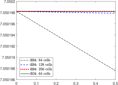
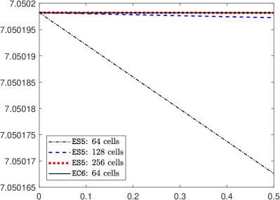
Figure 1: Example 6: Evolution of discrete total entropy.

[1D Riemann problems]This example verifies the performance of the proposed entropy conservative and entropy stable schemes in resolving 1D RMHD wave configurations, by simulating four 1D Riemann problems (RPs) [3, 39]. The initial data of each RP comprise two different constant states separated by the initial discontinuity at $x=0$, see Table 3. Their exact solutions were provided in [33].

Table 3: Initial data of the four 1D RPs in Example 1.

		$\rho$	$v_{1}$	$v_{2}$	$v_{3}$	$B_{1}$	$B_{2}$	$B_{3}$	$p$
RP I	left state	1.08	0.4	0.3	0.2	2	0.3	0.3	0.95
	right state	1	-0.45	-0.2	0.2	2.0	-0.7	0.5	1
RP II	left state	1	0	0	0	5	6	6	30
	right state	1	0	0	0	5	0.7	0.7	1
RP III	left state	1	0	0.3	0.4	1	6	2	5
	right state	0.9	0	0	0	1	5	2	5.3
RP IV	left state	1	0	0	0	0	2	0	10
	right state	0.1	0	0	0	0	0	0	1

Figures 2, 3 and 4 give the numerical results obtained by using ES5 with $1000$ uniform cells for RPs I, II and III, respectively. We see that the wave structures including discontinuities are well resolved by ES5 and that the numerical solutions are in good agreement with the exact ones.

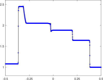
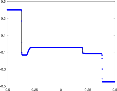
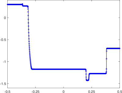
Figure 2: The first Riemann problem in Example 1: The density $\rho$ (top-left), velocity $v_{1}$ (top-right), magnetic field component $B_{2}$ (bottom-left), and pressure $p$ (bottom-right) at $t=0.55$. The symbols “${\color[rgb]{0,0,1}\circ}$” denote the numerical solutions computed by ES5, while the solid lines denote the exact solutions.

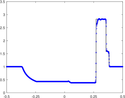
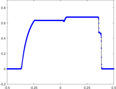
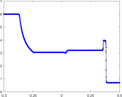
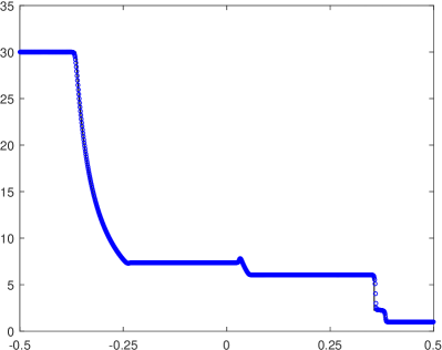
Figure 3: Same as Figure 2 except for the second Riemann problem at $t=0.4$.

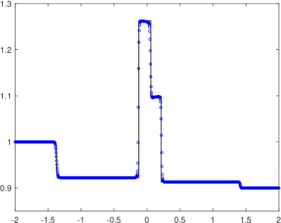
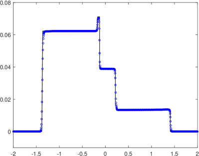
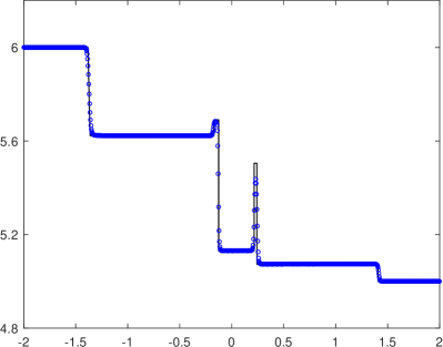
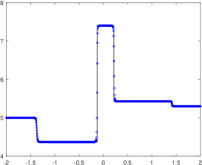
Figure 4: Same as Figure 2 except for the third Riemann problem at $t=1.5$.

The RP IV is a variant of the RMHD shock-tube 2 proposed by Komissarov [39] with $\Gamma=\frac{4}{3}$. The numerical solutions at $t=1$, computed respectively by EC6 and ES5 on $1000$ uniform girds, are displayed in Figure 5. We see that EC6 produces high-frequency oscillations in its numerical solution, because it enforces entropy conservation so that the entropy dissipation at the shock does not take place. Oscillations are not produced in the numerical solution of ES5, owing to its WENO dissipative mechanism. In order to carefully verify the entropy conservative/stable property of the proposed schemes, we investigate the behavior of the discrete total entropy ${\mathcal{E}}_{\rm tot}(t):=\sum_{i}{\mathcal{E}}({\bf U}_{i}(t))\Delta x$. Figure 6 shows the evolution of ${\mathcal{E}}_{\rm tot}(t)$ computed by EC6 and ES5, respectively, with fourth-order TVD explicit Runge-Kutta time discretization and different CFL numbers (correspond to different time step-sizes). For ES5, we see that the entropy dissipates at almost the same rates for different time step-sizes, as expected. Although the semi-discrete scheme EC6 conserves the entropy in theory, the results of the fully discrete scheme show small-magnitude entropy dissipation, which is solely introduced by time discretization. This is evidenced by the observation that the dissipation magnitude for EC6 becomes smaller when smaller CFL numbers are used. To further verify that the entropy conservative property converges in time with the temporal order, we show the logarithmic plots of the decrement of the total entropy in Figure 7. Again, Figure 7(a) clearly shows that the decrement magnitude becomes smaller for smaller time step-sizes. Moreover, Figure 7(b) indicates that the entropy dissipates at a rate of order ${\mathcal{O}}(\Delta t^{5})$, ranging from $\sim 10^{-3}$ with ${\rm CFL}=0.4$ to $\sim 10^{-8}$ with ${\rm CFL}=0.05$. This demonstrates the convergence of the entropy conservative property and confirms that the semi-discrete scheme EC6 does conserve entropy.

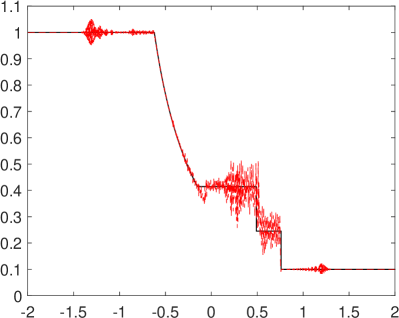
(a) Entropy conservative scheme EC6

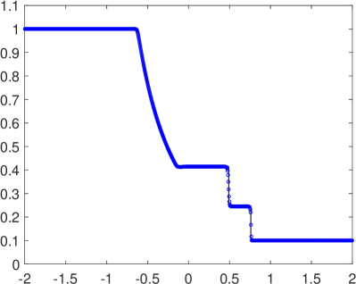
(b) Entropy stable scheme ES5

Figure 5: The density $\rho$ at $t=1$ for RP IV in Example 1. The dash line and the symbols “${\color[rgb]{0,0,1}\circ}$” denote the numerical solutions computed by EC6 and ES5, respectively, while the solid lines denote the exact solutions obtained by the RP solver in [33].

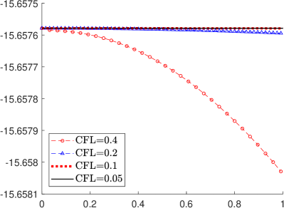
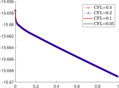
Figure 6: Time evolution of discrete total entropy for EC6 (left) and ES5 (right) with fourth-order TVD Runge-Kutta time discretization and different CFL numbers.

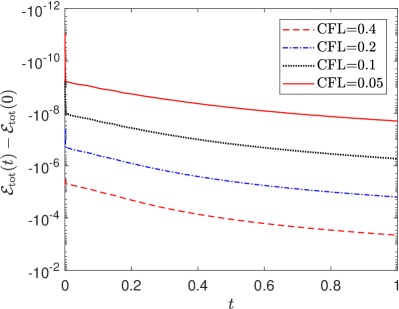
(a) Evolution of ${\mathcal{E}}_{\rm tot}(t)-{\mathcal{E}}_{\rm tot}(0)$

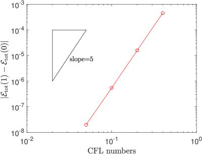
(b) Decrement $|{\mathcal{E}}_{\rm tot}(1)-{\mathcal{E}}_{\rm tot}(0)|$ at $t=1$

Figure 7: The decrement of total entropy for EC6 with fourth-order TVD Runge-Kutta time discretization and different CFL numbers.

[Blast problem]Blast problem is a benchmark test for RMHD numerical schemes. Our setup is the same as in [45, 67]. Initially, the computational domain $[-6,6]^{2}$ is filled with a homogeneous gas at rest with adiabatic index $\Gamma=4/3$. The explosion zone ($r<0.8$) has a density of $10^{-2}$ and a pressure of $1$, while the ambient medium ($r>1$) has a low density of $10^{-4}$ and a low pressure of $5\times 10^{-4}$, where $r=\sqrt{x^{2}+y^{2}}$. A linear taper is applied to the density and pressure for $r\in[0.8,1]$. The magnetic field is initialized in the $x$-direction as $0.1$.

Our numerical results at $t=4$, obtained by using ES5 on the mesh of $400\times 400$ uniform cells, are shown in Figure 8. We observe that the wave pattern of the configuration is composed by two main waves, an external fast and a reverse shock waves. The former is almost circular, while the latter is somewhat elliptic. The magnetic field is essentially confined between them, while the inner region is almost devoid of magnetization. Our numerical results agree quite well with those reported in [67, 66]. To validate the entropy stability of ES5, we compute the total entropy $\sum_{i,j}{\mathcal{E}}({\bf U}_{ij}(t))\Delta x\Delta y$, which should decrease with time if the scheme is entropy stable. The evolution of total entropy is displayed in the left of Figure 10 obtained by using ES5 at different gird resolutions. We clearly see a monotonic decay which indicates that the fully discrete scheme ES5 is entropy stable.

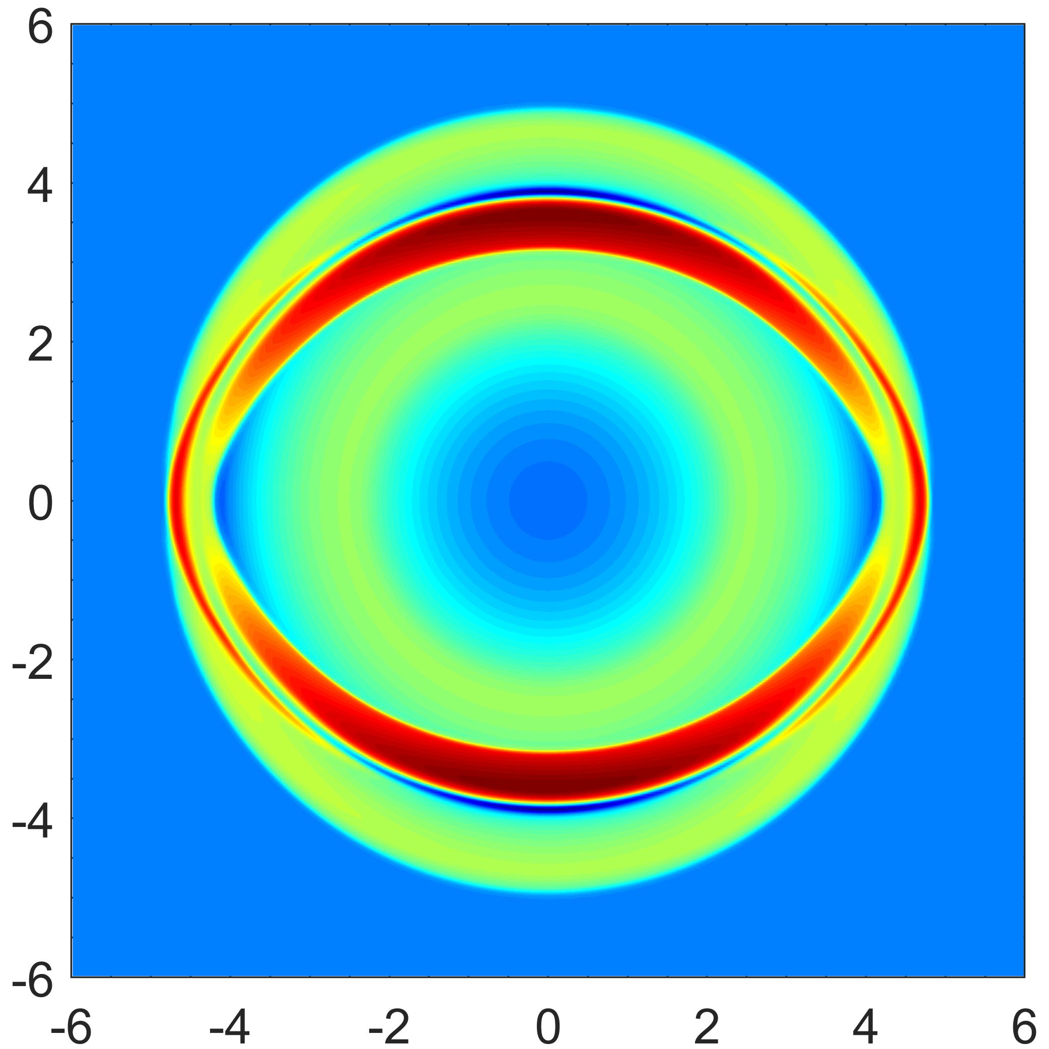
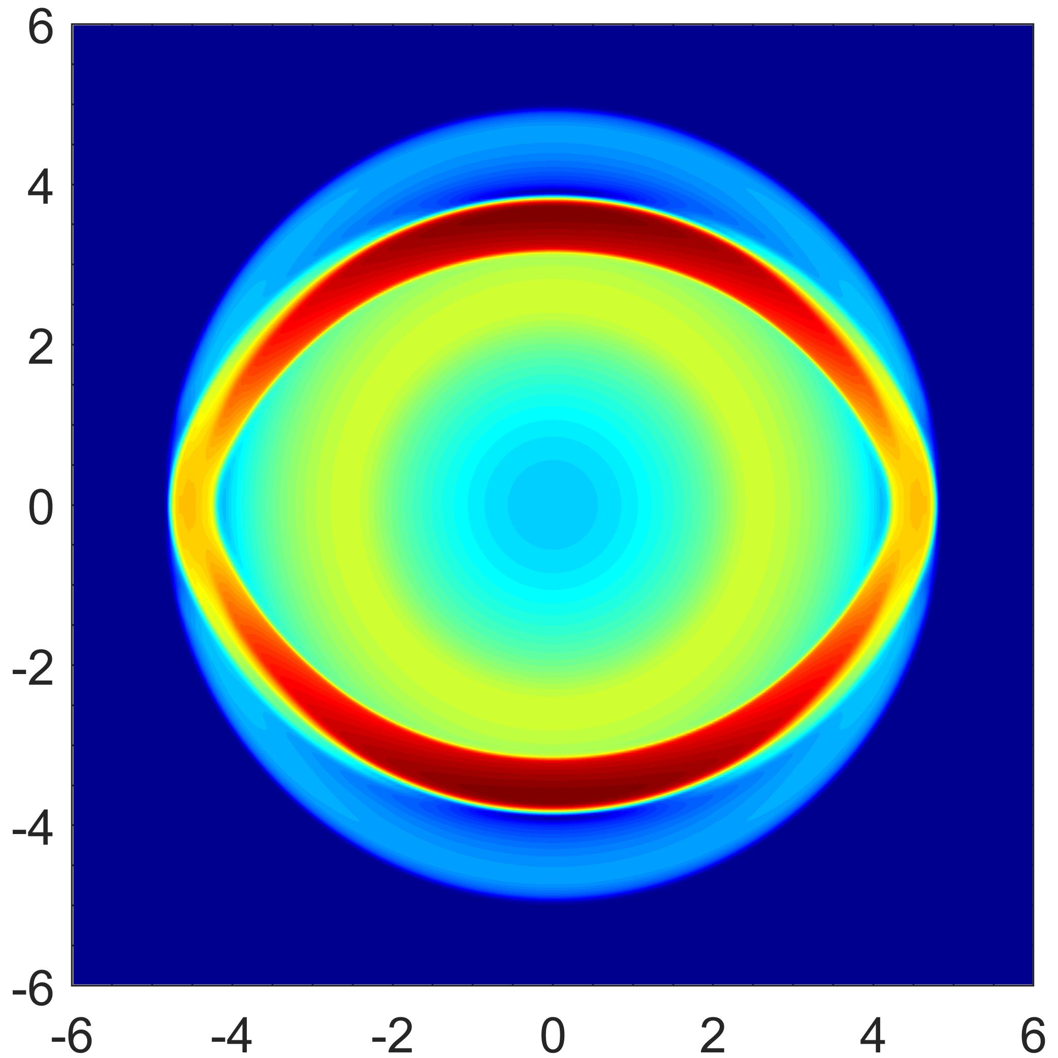
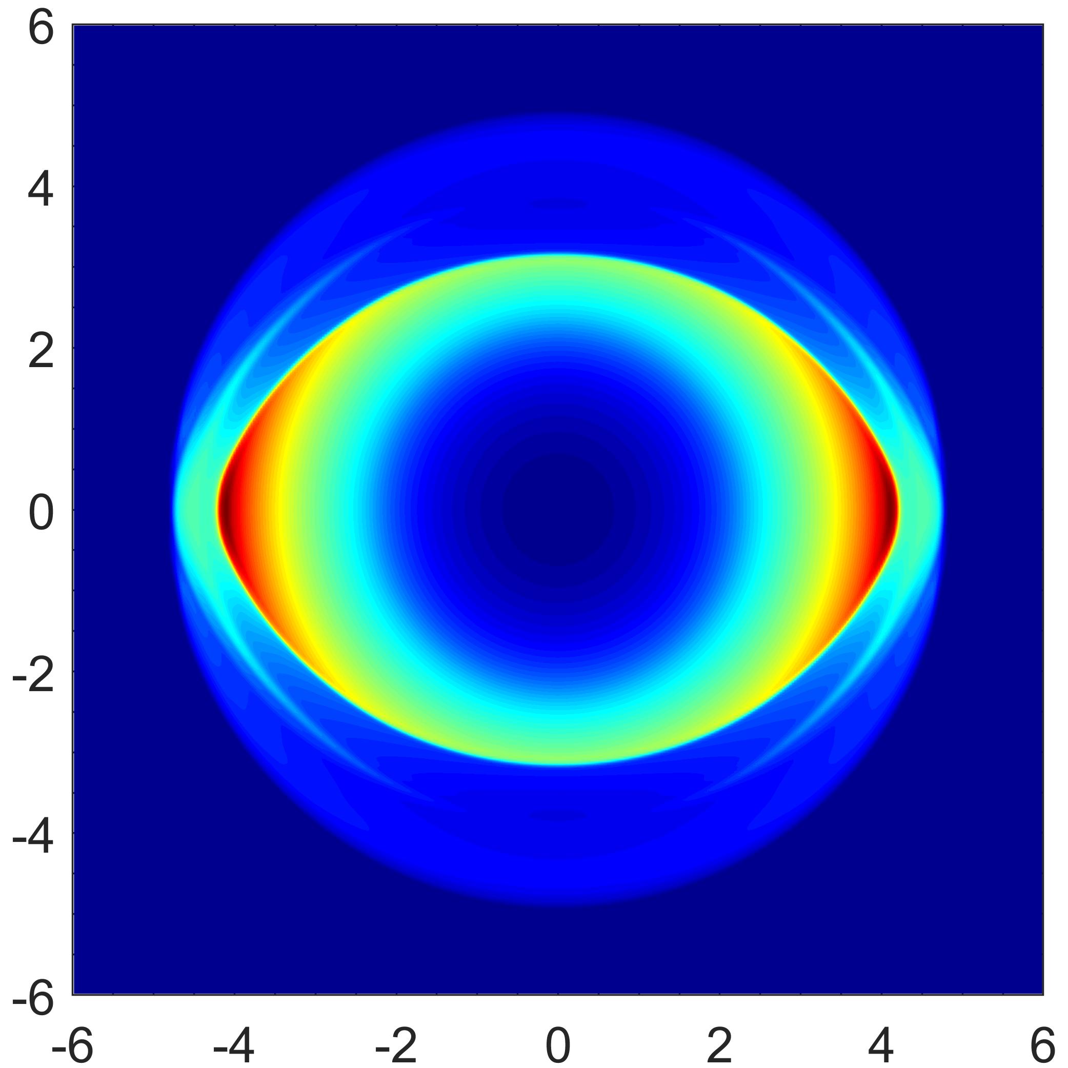
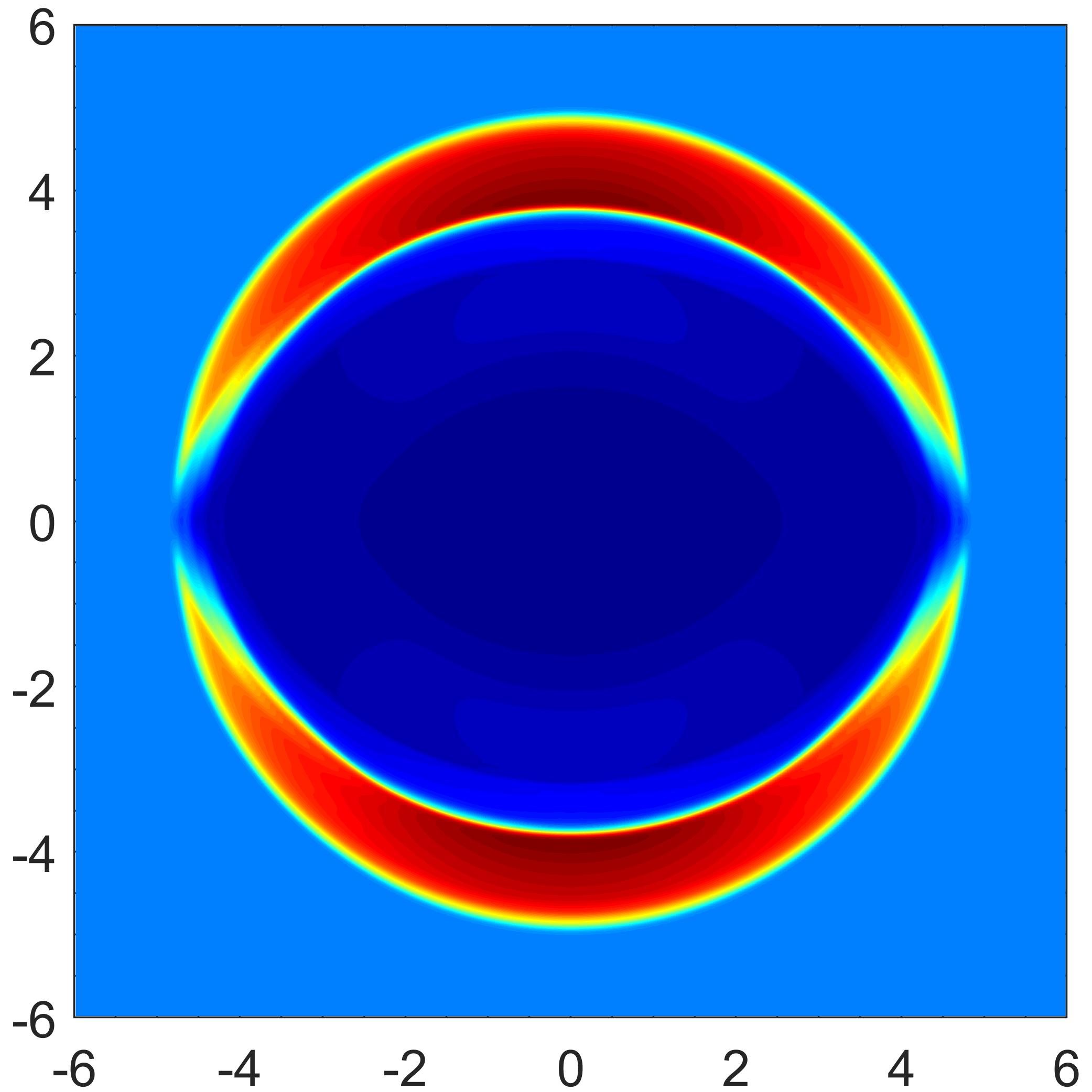
Figure 8: Example 7: the schlieren images of density logarithm (top-left), gas pressure (top-right), Lorentz factor (bottom-left) and magnetic field strength (bottom-right) at $t=4$.

[Orszag-Tang problem]This test simulates the relativistic version [58] of the classical Orszag-Tang problem [46]. Our setup is the same as in [58]. Initially, the computational domain $[0,2\pi]^{2}$ is filled with hot gas. We set the adiabatic index $\Gamma=4/3$, the initial pressure $p=10$, and the rest-mass density $\rho=1$. The initial velocity field of the fluid is given by ${\bf v}(x,y,0)=(-A\sin(y),A\sin(x),0)^{\top},$ where the parameter $A=0.99/\sqrt{2}$ so that the maximum velocity is $0.99$ (the corresponding Lorentz factor is about $7$). The magnetic field is initialized at ${\bf B}(x,y,0)=(-\sin y,\sin(2x),0)^{\top}$. Periodic conditions are specified at all the boundaries. Although the solution of this problem is smooth initially, complicated wave structures are formed as the time increases, and turbulence behavior will be produced eventually.

Figure 9 gives the numerical results obtained by using ES5 on $600\times 600$ uniform grids. In comparison with the results in [58], the complicated flow structures are well captured by ES5 with high resolution. To validate the entropy stability, the evolution of total entropy is shown in the right of Figure 10 obtained by using ES5 at different gird resolutions. We observe that the total entropy remains constant at initial times because initially the solution is smooth, and it starts to decrease at $t\approx 2$ when discontinuities start to form, as expected.

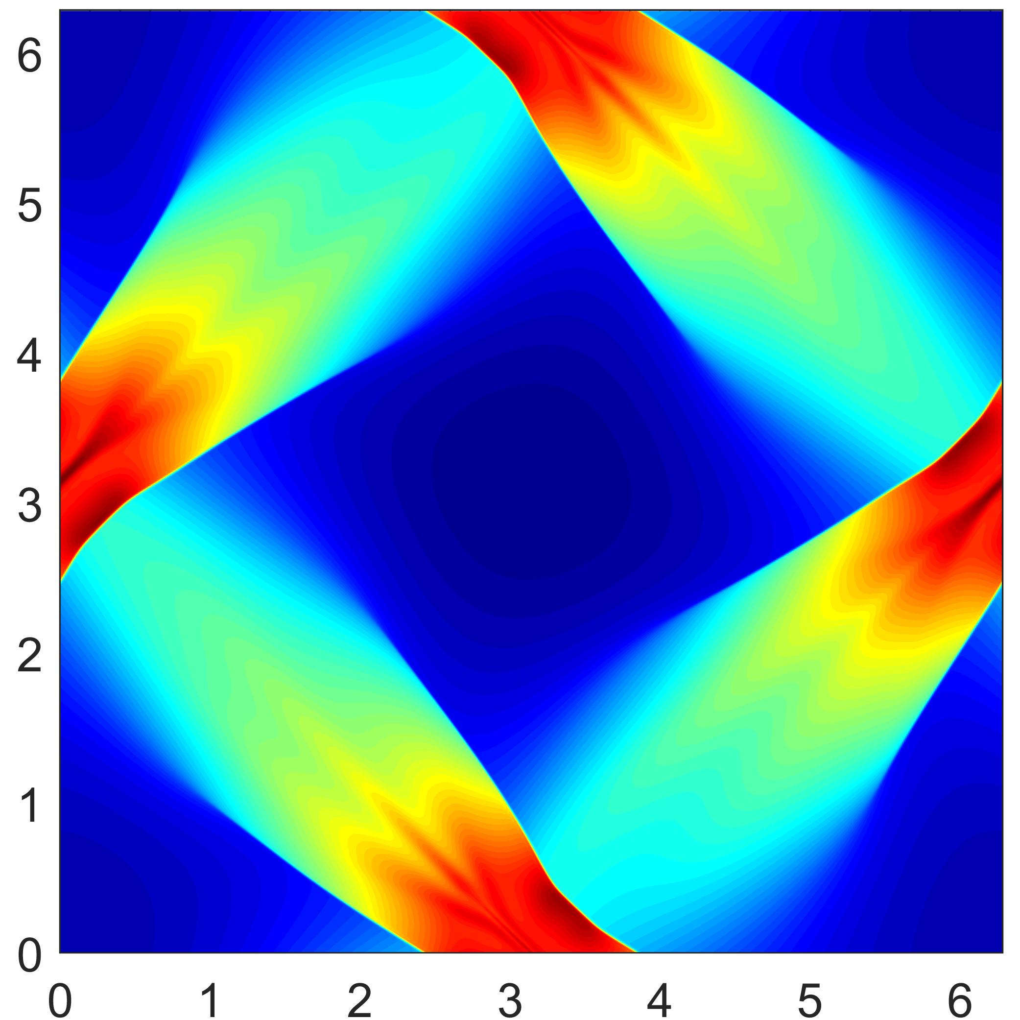
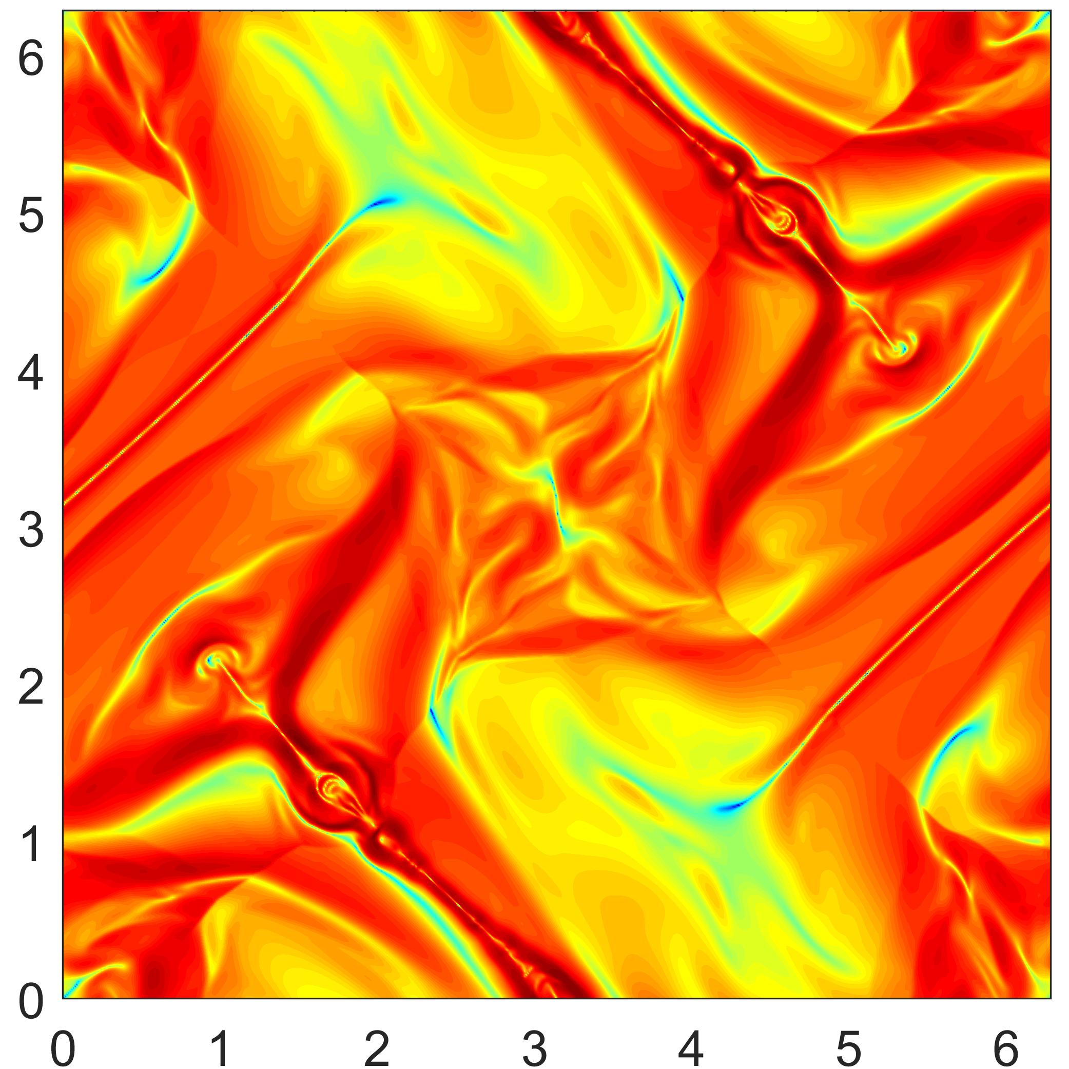
Figure 9: Example 8: the schlieren images of rest-mass density logarithm (left) and magnetic pressure logarithm (right). Top: $t=2.818127$; bottom: $t=6.8558$.

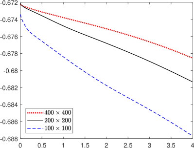
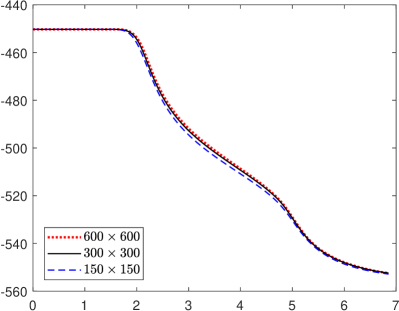
Figure 10: Evolution of total entropy for the blast problem (left) and the Orszag-Tang problem (right), obtained by using ${\tt ES5}$ at different grid resolutions.

[Shock cloud interaction problem]This problem describes the disruption of a high density cloud by a strong shock wave. Our setup is the same as in [35]. The computational domain is $[-0.2,1.2]\times[0,1]$, with the left boundary specified as inflow condition and the others as outflow conditions. Initially, a shock wave moves to the right from $x=0.05$, with the left and right states

$${{\bf V}}_{L}=(3.86859,0.68,0,0,0,0.84981,-0.84981,1.25115)^{\top},$$

$${{\bf V}}_{R}=(1,0,0,0,0,0.16106,0.16106,0.05)^{\top},$$

respectively. There exists a rest circular cloud centred at the point $(0.25,0.5)$ with radius 0.15. The cloud has the same states to the surrounding fluid except for a higher density of 30. Figure 11 displays the schlieren images of rest-mass density logarithm and magnetic pressure logarithm at $t=1.2$ obtained by using ES5 with $560\times 400$ uniform cells. One can see that the discontinuities are captured with high resolution, and the results agree well with those in [35, 68, 66].

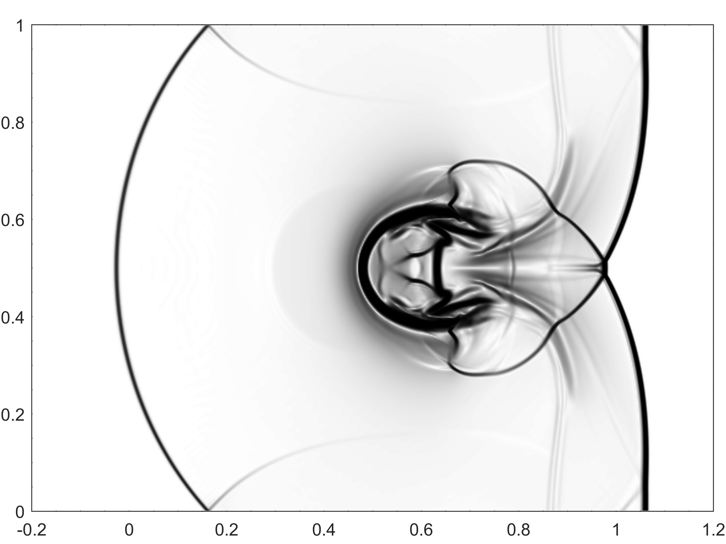
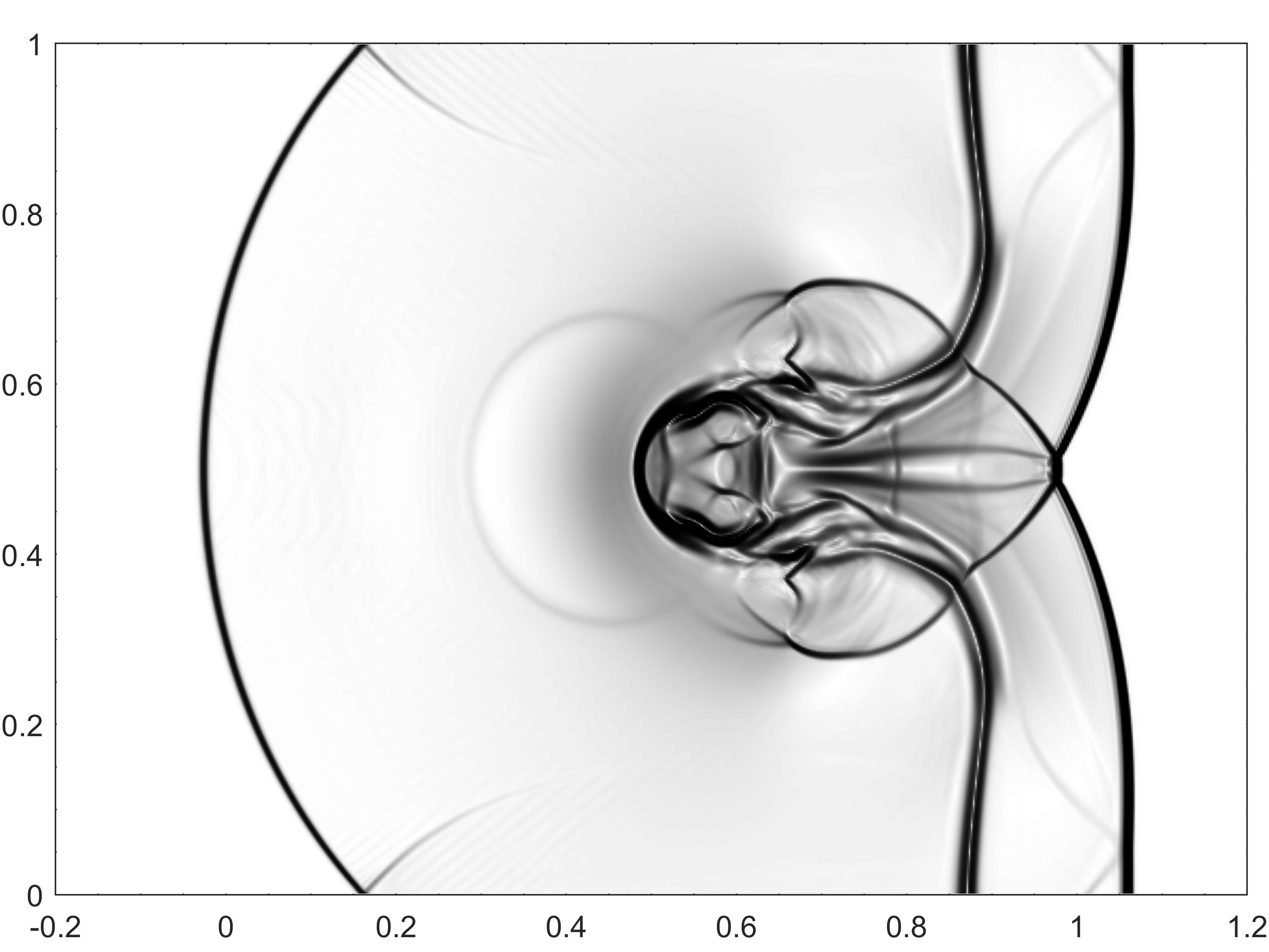
Figure 11: Example 10: the schlieren images of rest-mass density logarithm (left) and magnetic pressure logarithm (right) at time $t=1.2$.

7 Conclusions

In this paper, we presented rigorous entropy analysis and developed high-order accurate entropy stable schemes for the RMHD equations. We proved that the conservative RMHD equations (1) are not symmetrizable and thus do not admit an entropy pair. To address this issue, we first proposed a symmetrizable RMHD system (15) by building the divergence-free condition (2) into the RMHD equations through an additional source term. Based on the symmetrizable RMHD system, high-order accurate entropy stable finite difference schemes are developed on Cartesian meshes. These schemes are built on affordable explicit entropy conservative fluxes that are technically derived through carefully selected parameter variables, a special high-order discretization of the source term in the symmetrizable RMHD system, and suitable high-order dissipative operators based on (weighted) essentially non-oscillatory reconstruction to ensure the entropy stability. The accuracy and robustness of the proposed entropy stable schemes were demonstrated by benchmark numerical RMHD examples. The symmetrizable RMHD system is a relativistic analogue to the non-relativistic Godunov–Powell system [31, 49]. Its discovery would also enable one to generalize a large class of related numerical methods, including some other entropy stable schemes (e.g. [43]) and Powell’s eight-wave methods, to RMHDs.

References

- [1] A. Anile and S. Pennisi, On the mathematical structure of test relativistic magnetofluiddynamics, in Annales de l’IHP Physique théorique, vol. 46, 1987, pp. 27–44.
- [2] L. Antón, J. A. Miralles, J. M. Martí, J. M. Ibáñez, M. A. Aloy, and P. Mimica, Relativistic magnetohydrodynamics: renormalized eigenvectors and full wave decomposition Riemann solver, Astrophys. J. Suppl. Ser., 188 (2010), p. 1.
- [3] D. Balsara, Total variation diminishing scheme for relativistic magnetohydrodynamics, Astrophys. J. Suppl. Ser., 132 (2001), p. 83.
- [4] D. S. Balsara, Second-order-accurate schemes for magnetohydrodynamics with divergence-free reconstruction, Astrophys. J. Suppl. Ser., 151 (2004), pp. 149–184.
- [5] T. Barth, Numerical methods for gasdynamic systems on unstructured meshes, in An introduction to recent developments in theory and numerics for conservation laws, Springer, 1999, pp. 195–285.
- [6] T. Barth, On the role of involutions in the discontinuous Galerkin discretization of Maxwell and magnetohydrodynamic systems, in Compatible spatial discretizations, Springer, 2006, pp. 69–88.
- [7] B. Biswas and R. K. Dubey, Low dissipative entropy stable schemes using third order WENO and TVD reconstructions, Adv. Comput. Math., 44 (2018), pp. 1153–1181.
- [8] F. Bouchut, C. Bourdarias, and B. Perthame, A MUSCL method satisfying all the numerical entropy inequalities, Math. Comp., 65 (1996), pp. 1439–1461.
- [9] J. U. Brackbill and D. C. Barnes, The effect of nonzero on the numerical solution of the magnetodydrodynamic equations, J. Comput. Phys., 35 (1980), pp. 426–430.
- [10] M. H. Carpenter, T. C. Fisher, E. J. Nielsen, and S. H. Frankel, Entropy stable spectral collocation schemes for the Navier–Stokes equations: Discontinuous interfaces, SIAM J. Sci. Comput., 36 (2014), pp. B835–B867.
- [11] P. Chandrashekar, Kinetic energy preserving and entropy stable finite volume schemes for compressible Euler and Navier-Stokes equations, Commun. Comput. Phys., 14 (2013), pp. 1252–1286.
- [12] P. Chandrashekar and C. Klingenberg, Entropy stable finite volume scheme for ideal compressible MHD on 2-D Cartesian meshes, SIAM J. Numer. Anal., 54 (2016), pp. 1313–1340.
- [13] T. Chen and C.-W. Shu, Entropy stable high order discontinuous Galerkin methods with suitable quadrature rules for hyperbolic conservation laws, J. Comput. Phys., 345 (2017), pp. 427–461.
- [14] M. G. Crandall and A. Majda, Monotone difference approximations for scalar conservation laws, Math. Comp., 34 (1980), pp. 1–21.
- [15] C. M. Dafermos, Hyperbolic Conservation Laws in Continuum Physics, vol. 325, Springer, 4th ed., 2010.
- [16] A. Dedner, F. Kemm, D. Kröner, C.-D. Munz, T. Schnitzer, and M. Wesenberg, Hyperbolic divergence cleaning for the MHD equations, J. Comput. Phys., 175 (2002), pp. 645–673.
- [17] D. Derigs, A. R. Winters, G. J. Gassner, and S. Walch, A novel high-order, entropy stable, 3D AMR MHD solver with guaranteed positive pressure, J. Comput. Phys., 317 (2016), pp. 223–256.
- [18] D. Derigs, A. R. Winters, G. J. Gassner, S. Walch, and M. Bohm, Ideal GLM-MHD: About the entropy consistent nine-wave magnetic field divergence diminishing ideal magnetohydrodynamics equations, J. Comput. Phys., 364 (2018), pp. 420–467.
- [19] J. Duan and H. Tang, High-order accurate entropy stable finite difference schemes for one-and two-dimensional special relativistic hydrodynamics, arXiv:1905.06092, (2019).
- [20] C. R. Evans and J. F. Hawley, Simulation of magnetohydrodynamic flows: a constrained transport method, Astrophys. J., 332 (1988), pp. 659–677.
- [21] T. C. Fisher and M. H. Carpenter, High-order entropy stable finite difference schemes for nonlinear conservation laws: Finite domains, J. Comput. Phys., 252 (2013), pp. 518–557.
- [22] U. S. Fjordholm, S. Mishra, and E. Tadmor, Energy preserving and energy stable schemes for the shallow water equations, in Foundations of Computational Mathematics, Hong Kong 2008, vol. 363 of London Math. Soc. Lecture Notes Series, 2009, pp. 93–139.
- [23] U. S. Fjordholm, S. Mishra, and E. Tadmor, Arbitrarily high-order accurate entropy stable essentially nonoscillatory schemes for systems of conservation laws, SIAM J. Numer. Anal., 50 (2012), pp. 544–573.
- [24] U. S. Fjordholm, S. Mishra, and E. Tadmor, ENO reconstruction and ENO interpolation are stable, Found. Comput. Math., 13 (2013), pp. 139–159.
- [25] U. S. Fjordholm and D. Ray, A sign preserving WENO reconstruction method, J. Sci. Comput., 68 (2016), pp. 42–63.
- [26] J. A. Font, Numerical hydrodynamics and magnetohydrodynamics in general relativity, Living Rev. Relativ., 11 (2008), p. 7.
- [27] H. Freistühler and Y. Trakhinin, Symmetrizations of RMHD equations and stability of relativistic current–vortex sheets, Classical and Quantum Gravity, 30 (2013), p. 085012.
- [28] G. J. Gassner, A skew-symmetric discontinuous Galerkin spectral element discretization and its relation to SBP-SAT finite difference methods, SIAM J. Sci. Comput., 35 (2013), pp. A1233–A1253.
- [29] G. J. Gassner, A. R. Winters, and D. A. Kopriva, A well balanced and entropy conservative discontinuous Galerkin spectral element method for the shallow water equations, Appl. Math. Comput., 272 (2016), pp. 291–308.
- [30] E. Godlewski and P.-A. Raviart, Numerical approximation of hyperbolic systems of conservation laws, vol. 118, Springer Science & Business Media, 2013.
- [31] S. K. Godunov, Symmetric form of the equations of magnetohydrodynamics, Numerical Methods for Mechanics of Continuum Medium, 1 (1972), pp. 26–34.
- [32] F. Guercilena, D. Radice, and L. Rezzolla, Entropy-limited hydrodynamics: a novel approach to relativistic hydrodynamics, Comput. Astrophys. Cosmol., 4 (2017), p. 3.
- [33] F. Guercilena and L. Rezzolla, The exact solution of the Riemann problem in relativistic magnetohydrodynamics, J. Fluid Mech., 562 (2006), pp. 223–259.
- [34] A. Harten, J. M. Hyman, P. D. Lax, and B. Keyfitz, On finite-difference approximations and entropy conditions for shocks, Commun. Pure Appl. Math., 29 (1976), pp. 297–322.
- [35] P. He and H. Tang, An adaptive moving mesh method for two-dimensional relativistic magnetohydrodynamics, Comput. Fluids, 60 (2012), pp. 1–20.
- [36] J. S. Hesthaven and F. Mönkeberg, Entropy stable essentially nonoscillatory methods based on RBF reconstruction, ESAIM. Math. Model Numer. Anal., 53 (2019), pp. 925–958.
- [37] A. Hiltebrand and S. Mishra, Entropy stable shock capturing space–time discontinuous galerkin schemes for systems of conservation laws, Numer. Math., 126 (2014), pp. 103–151.
- [38] F. Ismail and P. L. Roe, Affordable, entropy-consistent Euler flux functions II: Entropy production at shocks, J. Comput. Phys., 228 (2009), pp. 5410–5436.
- [39] S. S. Komissarov, A Godunov-type scheme for relativistic magnetohydrodynamics, Mon. Not. R. Astron. Soc., 303 (1999), pp. 343–366.
- [40] P. G. Lefloch, J.-M. Mercier, and C. Rohde, Fully discrete, entropy conservative schemes of arbitrary order, SIAM J. Numer. Anal., 40 (2002), pp. 1968–1992.
- [41] F. Li and C.-W. Shu, Locally divergence-free discontinuous Galerkin methods for MHD equations, J. Sci. Comput., 22 (2005), pp. 413–442.
- [42] F. Li, L. Xu, and S. Yakovlev, Central discontinuous Galerkin methods for ideal MHD equations with the exactly divergence-free magnetic field, J. Comput. Phys., 230 (2011), pp. 4828–4847.
- [43] Y. Liu, C.-W. Shu, and M. Zhang, Entropy stable high order discontinuous Galerkin methods for ideal compressible MHD on structured meshes, J. Comput. Phys., 354 (2018), pp. 163–178.
- [44] J. M. Martí and E. Müller, Grid-based methods in relativistic hydrodynamics and magnetohydrodynamics, Living Rev. Comput. Astrophys., 1 (2015), p. 3.
- [45] A. Mignone and G. Bodo, An HLLC riemann solver for relativistic flows–II. magnetohydrodynamics, Mon. Not. R. Astron. Soc., 368 (2006), pp. 1040–1054.
- [46] S. A. Orszag and C.-M. Tang, Small-scale structure of two-dimensional magnetohydrodynamic turbulence, J. Fluid Mech., 90 (1979), pp. 129–143.
- [47] S. Osher, Riemann solvers, the entropy condition, and difference, SIAM J. Numer. Anal., 21 (1984), pp. 217–235.
- [48] S. Osher and E. Tadmor, On the convergence of difference approximations to scalar conservation laws, Math. Comp., 50 (1988), pp. 19–51.
- [49] K. G. Powell, An approximate Riemann solver for magnetohydrodynamics (that works in more than one dimension), Tech. Report ICASE Report No. 94-24, NASA Langley, VA, 1994.
- [50] K. G. Powell, P. Roe, R. Myong, and T. Gombosi, An upwind scheme for magnetohydrodynamics, in 12th Computational Fluid Dynamics Conference, 1995, p. 1704.
- [51] H. Ranocha, Comparison of some entropy conservative numerical fluxes for the euler equations, J. Sci. Comput., 76 (2018), pp. 216–242.
- [52] T. Ruggeri and A. Strumia, Convex covariant entropy density, symmetric conservative form, and shock waves in relativistic magnetohydrodynamics, J. Math. Phys., 22 (1981), pp. 1824–1827.
- [53] E. Tadmor, The numerical viscosity of entropy stable schemes for systems of conservation laws. I, Math. Comp., 49 (1987), pp. 91–103.
- [54] E. Tadmor, Entropy stability theory for difference approximations of nonlinear conservation laws and related time-dependent problems, Acta Numer., 12 (2003), pp. 451–512.
- [55] E. Tadmor and W. Zhong, Entropy stable approximations of Navier–Stokes equations with no artificial numerical viscosity, J. Hyperbolic Differ. Equ., 03 (2006), pp. 529–559.
- [56] G. Tóth, The constraint in shock-capturing magnetohydrodynamics codes, J. Comput. Phys., 161 (2000), pp. 605–652.
- [57] Y. L. Trakhinin, On stability of shock waves in relativistic magnetohydrodynamics, Quarterly of Applied Mathematics, 59 (2001), pp. 25–45.
- [58] B. van der Holst, R. Keppens, and Z. Meliani, A multidimensional grid-adaptive relativistic magnetofluid code, Comput. Phys. Commun., 179 (2008), pp. 617–627.
- [59] M. H. van Putten, Maxwell’s equations in divergence form for general media with applications to MHD, Commun. Math. Phys., 141 (1991), pp. 63–77.
- [60] M. H. van Putten, A two-dimensional numerical implementation of magnetohydrodynamics in divergence form, SIAM J. Numer. Anal., 32 (1995), pp. 1504–1518.
- [61] M. H. van Putten, Knots in simulations of magnetized relativistic jets, Astrophys. J. Lett., 467 (1996), p. L57.
- [62] A. R. Winters and G. J. Gassner, Affordable, entropy conserving and entropy stable flux functions for the ideal MHD equations, J. Comput. Phys., 304 (2016), pp. 72–108.
- [63] K. Wu, Positivity-preserving analysis of numerical schemes for ideal magnetohydrodynamics, SIAM J. Numer. Anal., 56 (2018), pp. 2124–2147.
- [64] K. Wu and C.-W. Shu, A provably positive discontinuous Galerkin method for multidimensional ideal magnetohydrodynamics, SIAM J. Sci. Comput., 40 (2018), pp. B1302–B1329.
- [65] K. Wu and C.-W. Shu, Provably positive high-order schemes for ideal magnetohydrodynamics: analysis on general meshes, Numer. Math., 142 (2019), pp. 995–1047.
- [66] K. Wu and H. Tang, Admissible states and physical-constraints-preserving schemes for relativistic magnetohydrodynamic equations, Math. Models Methods Appl. Sci., 27 (2017), pp. 1871–1928.
- [67] O. Zanotti, F. Fambri, and M. Dumbser, Solving the relativistic magnetohydrodynamics equations with ADER discontinuous Galerkin methods, a posteriori subcell limiting and adaptive mesh refinement, Mon. Not. R. Astron. Soc., 452 (2015), pp. 3010–3029.
- [68] J. Zhao and H. Tang, Runge-Kutta discontinuous Galerkin methods for the special relativistic magnetohydrodynamics, J. Comput. Phys., 343 (2017), pp. 33–72.