Adapting the Teubner reciprocal relations for stokeslet objects

Abstract

Self-propelled colloidal swimmers move by pushing the adjacent fluid backwards. The resulting motion of an asymmetric body depends on the profile of pushing velocity over its surface. We describe a method of predicting the motion arising from arbitrary velocity profiles over a given body shape, using a discrete-source “stokeslet” representation. The net velocity and angular velocity is a sum of contributions from each point on the surface. The contributions from a given point depend only on the shape. We give a numerical method to find these contributions in terms of the stokeslet positions defining the shape. Each contribution is determined by linear operations on the Oseen interaction matrix between pairs of stokeslets. We first adapt the Lorentz Reciprocal Theorem to discrete sources. We then use the theorem to implement the method of TeubnerTeubner (1982) to determine electrophoretic mobilities of nonuniformly charged bodies.

I Introduction

Many forms of propulsion of microscopic objects through fluids work via phoresis: the surface of the object pushes the adjacent fluid to create a thin slip layer of nonzero relative velocityMoran and Posner (2017). Electrophoresis in an ionic fluid is a prime example; thermophoresis and chemophoresis behave analogouslyAnderson (1989); Stone and Samuel (1996); Eslahian et al. (2014); Moyses et al. (2016). In active propulsion chemical reactions at the surface create the propulsive surface flowWalther and Müller (2013); Maass et al. (2016). Similarly many living organisms propel themselves via a layer of beating cilia on the surfaceMarchetti et al. (2013). Even when the profile of the slip velocity is known, determining the resulting motion is challenging, especially when the object has an asymmetric shape. Here we describe a general method of determining motion of an asymmetric self-propelling object.

We describe this method in the important context of electrophoretic motion of a body of given shape and charge distributionAnderson (1989, 1985); Fair and Anderson (1989); Long and Ajdari (1998); Chae and Lenhoff (1995); Allison (2001); Delgado et al. (2007). On one level these motions amount to a mere linear response. Yet the motions can be complex and unintuitive. The body may rotate steadily with no electrophoretic translation; it may translate perpendicular to the applied fieldLong and Ajdari (1998). The body may move with an intrinsic chirality even though its shape is not chiral. Analogous sedimentary motions were shown to enable coherent control over a dispersion of like objectsMoths and Witten (2013).

In recent times the experimental importance of such objects has steadily risen. Increasingly experiments study dispersions of colloidal particles of a common, asymmetric shapeHan et al. (2016); Sacanna et al. (2011); Meng et al. (2010). These bodies may be unevenly charged. The ability to manipulate such bodies by harnessing their asymmetry is increasingly desirable. Accordingly, there is an increasing need to predict the distinctive motions for a given shape and charge distribution. Current methods of making such predictions are ungainly or limited in scopeTeubner (1982); Delgado et al. (2007).

In 1982 TeubnerTeubner (1982); Burelbach and Stark (2019) made an insightful simplification of this problem. He showed that the influence of charge distribution on a given body could be distilled into a set of six functions defined over its surface. Each function amounted to the distribution of hydrodynamic shear stress over that surface when certain specified motions were imposed. Using these six functions one may find the motion of the given body with arbitrary charge distributions. His findings exploited the long-known Lorentz Reciprocal relations for stokes flow Happel and Brenner (1983). However, finding these functions requires solving the Stokes equations for the fluid around the body in arbitrary motion. Predicting the motion also required determining the applied electric field over the surface.

One may avoid dealing with these equations by approximating the body as a “stokeslet object”. A stokeslet object is defined by a set of $N$ point sources or stokeslets $i$ applied at fixed relative positions $\vec{r}_{i}$ in a fluid. Any force $\vec{f}_{i}$ on a stokeslet causes a proportional flow around $\vec{r}_{i}$ given by a $3\times 3$ response tensor $\mathsf{L\kern-4.0ptL}$ discussed below. A solid body can be approximated as a stokeslet object by replacing the body with a large number of stokeslets distributed over its surfaceMowitz and Witten (2017). By giving the stokeslets electric charge as well as hydrodynamic forcing, this approximation was shown to predict electrophoretic mobility successfully in simple casesMowitz and Witten (2017); Braverman et al. .

This stokeslet approach raises a question: What is the analog of Teubner’s insight for stokeslet objects? That is, what is the analog of the six functions that allow treatment of arbitrary charge distributions on the object? Here we answer this question and determine the analogous functions. This approach provides a simple complement to the differential equations of the Teubner theory.

The stokeslet approach also allows a simple understanding of the Lorentz Reciprocal Theorem Happel and Brenner (1983). This theorem applies to flow fields in a region confined by defined boundaries of some given shape and differing in the stresses at these boundaries. It follows from the multilinearity of the flow to the stress and the equality of external work and viscous dissipation. These same features dictate the linear response of the velocity field to a point source of force, or stokeslet. As in the Lorentz Reciprocal Theorem, the linear relation between the stokeslet forces and their velocity fields shows how two different velocity fields interact.

First, we recall how stokeslets create velocity fields. Next, we formulate the analog of the Lorentz Reciprocal relationHappel and Brenner (1983) for stokeslet objects. Finally, we apply this reciprocal relation to derive expressions for the force, torque and motion of an arbitrarily charged stokeslet object in an electric field.

II superposition of stokeslet responses

In the Stokes regime Happel and Brenner (1983) of weak flow in a fluid at rest at infinity, the velocity field of the fluid $\vec{v}(\vec{r})$ is a linear function of the external forces acting on it. A point force $\vec{f}_{j}$ acting at a position $\vec{r}_{j}$ produces a velocity field $\vec{v}_{j}(\vec{r})$ proportional to $\vec{f}_{j}$. That is,

$$\vec{v}_{j}(\vec{r})=\mathsf{L\kern-4.0ptL}(\vec{\Delta}r)\cdot\vec{f}_{j},$$ (1)

where $\mathsf{L\kern-4.0ptL}(\vec{\Delta}r)$ is a $3\times 3$ linear response tensor that depends on the displacement $\vec{r}-\vec{r}_{j}\equiv\vec{\Delta}r$ and the fluid’s viscosity. We note that this $\vec{v}_{j}(\vec{r})$ does not depend on any assumed motion of the forcing point $\vec{r}_{j}$ itself. Sec. VI.3 discusses the physical motion leading to the $\vec{f}_{j}$.

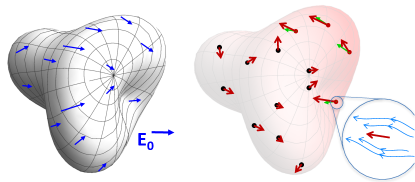
Figure 1: Electrophoresis of a partially charged stokeslet object. Left: object in an external field $\vec{E}_{0}$ pointing to the right. Colored arrows show tangential surface field $\vec{E}{\scriptscriptstyle\mathbf{S}}$, depending only on shape. Right: stokeslet representation of the object. Large dots show the stokeslet positions. Colored dots represent charged regions. Green, light arrows show slip velocity at the colored dots, proportional to $\vec{E}{\scriptscriptstyle\mathbf{S}}$ and to the local zeta potential $\zeta_{i}$. Red, heavy arrows show stokeslet forces that together produce matching velocities at the colored dots and zero velocity at the black dots. They also generally create flow in the interior. This flow is not relevant for electrophoretic motion. Inset at right: colored streamlines indicate the Oseen velocity field $\mathsf{L\kern-4.0ptL}(r)\cdot\vec{f}_{i}$ around one stokeslet.

We consider a given set of $N$ stokeslets at positions $\vec{r}_{1},\vec{r}_{2},...,\vec{r}_{N}=\{\vec{r}_{i}\}$. If forces $\{\vec{f}_{i}\}$ are applied to these stokeslets, a velocity field $\vec{v}(\vec{r})$ results, as shown in Fig.1. In particular, the velocity of the fluid at stokeslet $i$ is the sum of contributions $\vec{v}_{ij}$ due to the $\vec{f}_{j}$ via Eq. (1).

$$\vec{v}_{ij}=\mathsf{L\kern-4.0ptL}_{ij}\cdot\vec{f}_{j},$$ (2)

where $\mathsf{L\kern-4.0ptL}_{ij}\equiv\mathsf{L\kern-4.0ptL}(\vec{r}_{i}-\vec{r}_{j})$. The $\{\vec{v}_{i}\}$ are then determined by superposition:

$$\vec{v}_{i}=\sum_{j=1}^{N}\vec{v}_{ij}=\sum_{j=1}^{N}\mathsf{L\kern-4.0ptL}_{ij}\cdot\vec{f}_{j}$$ (3)

One may determine the $\{\vec{f}_{i}\}$ that generate a desired $\{\vec{v}_{i}\}$ by solving the $N$ simultaneous linear equations of Eq. (3) .

Together, the $\{\vec{v}_{i}\}$ and $\{\vec{f}_{i}\}$ determine the rate $\dot{W}$ at which the stokeslet forces do work on the fluid. This work is necessarily quadratic in the $\{\vec{f}_{i}\}$ When the stokeslets are placed together in the fluid, extra work is required for each stokeslet $i$ due to the velocity $v_{i}$ there due to the other stokeslets. The power $\dot{w}_{ij}$ associated with $\vec{f}_{i}$ and $\vec{f}_{j}$ is $\vec{f}_{i}\cdot\vec{v}_{ji}+\vec{f}_{j}\cdot\vec{v}_{ij}$ or

$$\vec{f}_{i}\cdot\mathsf{L\kern-4.0ptL}_{ij}\cdot\vec{f}_{j}+\vec{f}_{j}\cdot\mathsf{L\kern-4.0ptL}_{ji}\cdot\vec{f}_{i}=\vec{f}_{i}\cdot(\mathsf{L\kern-4.0ptL}_{ij}+\mathsf{L\kern-4.0ptL}_{ji}^{T})\cdot\vec{f}_{j}.$$ (4)

Here $\mathsf{L\kern-4.0ptL}_{ij}^{T}$ denotes the transpose of the 3$\times$3 matrix $\mathsf{L\kern-4.0ptL}_{ij}$.

This expression implies that the response tensor $\mathsf{L\kern-4.0ptL}$ itself is symmetric; that is, $\mathsf{L\kern-4.0ptL}_{ji}^{T}=\mathsf{L\kern-4.0ptL}_{ij}$. To verify this, we write $\mathsf{L\kern-4.0ptL}_{ij}$ as the sum of its symmetric and antisymmetric parts, $\mathsf{L\kern-4.0ptL}_{ij}^{S}\equiv\frac{1}{2}(\mathsf{L\kern-4.0ptL}_{ij}+\mathsf{L\kern-4.0ptL}_{ji}^{T})$ and $\mathsf{L\kern-4.0ptL}_{ij}^{A}\equiv\frac{1}{2}(\mathsf{L\kern-4.0ptL}_{ij}-\mathsf{L\kern-4.0ptL}_{ji}^{T})$. Eq. (4) shows that the $\dot{w}_{ij}$ depend on only the symmetric part $\mathsf{L\kern-4.0ptL}^{S}$, while the velocities $\vec{v}_{ij}$ are the sum of contributions from both $\mathsf{L\kern-4.0ptL}^{S}$ and $\mathsf{L\kern-4.0ptL}^{A}$. Thus if $\mathsf{L\kern-4.0ptL}^{A}$ were nonzero, it would give rise to a nonzero $\{\vec{v}_{i}\}$ whose $\dot{w}_{ij}=0$. Now, no such flow can exist, since every flow that vanishes at infinity necessarily has a nonzero shear rate and thence a positive $\dot{W}$ from viscous dissipation. Thus $\mathsf{L\kern-4.0ptL}^{A}$ vanishes and $\mathsf{L\kern-4.0ptL}$ is symmetric, as claimed.

III reciprocity

The symmetry of the response matrix $\mathsf{L\kern-4.0ptL}$ entails a reciprocal relation between different forces $\{\vec{f}_{i}\}$ and the velocities $\{\vec{v}_{i}\}$ they generate. This is the stokeslet analog of the Lorentz Reciprocal RelationHappel and Brenner (1983).

We now suppose that a given set of stokeslets experiences two sets of forces: $\{\vec{f}_{i}\}$ and $\{\vec{g}_{i}\}$. The $\{\vec{f}_{i}\}$ generate a set of velocities $\{\vec{v}_{i}\}$ as told above. Likewise, the $\{\vec{g}_{i}\}$ generate a different set of velocities denoted $\{\vec{u}_{i}\}$. Evidently part of the power $\dot{W}$ is the contribution from the forces $\{\vec{g}_{i}\}$ acting on the velocities $\{\vec{v}_{i}\}$: i.e. $\sum_{i}\vec{g}_{i}\cdot\vec{v}_{i}$. Another part is the contribution from the $\{\vec{f}_{i}\}$’s acting on the $\{\vec{u}_{i}\}$’s. Owing to the symmetry of $\mathsf{L\kern-4.0ptL}$, these two works can be readily seen to be equal: both are equal to a symmetric sum over $\{\vec{f}_{i}\}$ and $\{\vec{g}_{i}\}$:

$$\sum_{i=1}^{N}\vec{g}_{i}\cdot\vec{v}_{i}= \sum_{i,j=1}^{N}\vec{g}_{i}\cdot\mathsf{L\kern-4.0ptL}_{ij}\cdot\vec{f}_{j}=\sum_{i,j=1}^{N}\vec{f}_{j}\cdot\mathsf{L\kern-4.0ptL}^{T}_{ij}\cdot\vec{g}_{i}$$

$$= \sum_{i,j=1}^{N}\vec{f}_{j}\cdot\mathsf{L\kern-4.0ptL}_{ji}\cdot\vec{g}_{i}=\sum_{j=1}^{N}\vec{f}_{j}\cdot\vec{u}_{j}.$$ (5)

Thus the work done by $\{\vec{f}_{i}\}$ on the $\{\vec{g}_{i}\}$ velocities is equal to the work done by $\{\vec{g}_{i}\}$ on the $\{\vec{f}_{i}\}$ velocities.

IV electrophoretic forces

We may use this reciprocal relationship to determine the forces on a charged colloidal body in a static electric field $\vec{E}_{0}$. A body that is held stationary experiences a constraint force $\vec{F}$ and torque $\vec{\tau}$ proportional to $\vec{E}_{0}$. To lowest order in $E_{0}$ the force and torque are given by two tensors $\mathsf{K\kern-6.0ptK}_{F}$ and $\mathsf{K\kern-6.0ptK}_{\tau}$ defined by

$$\vec{F}=\mathsf{K\kern-6.0ptK}_{F}\cdot\vec{E}_{0}\quad\hbox{and}\quad\vec{\tau}=\mathsf{K\kern-6.0ptK}_{\tau}\cdot\vec{E}_{0}.$$ (6)

We consider the typical case in which ions in the solvent strongly screen any electric field due to the body charges $q_{i}$. Thus the field from the body charge is confined to a screening layer much thinner than the body’s sizeAnderson (1985). When the external field $\vec{E}_{0}$ is applied, the field near the insulating object is distorted, leaving a tangential surface field $\vec{E}{\scriptscriptstyle\mathbf{S}}(\vec{r})$ at the surface induced by $\vec{E}_{0}$. This $\vec{E}{\scriptscriptstyle\mathbf{S}}$ is caused by $\vec{E}_{0}$ alone, and it depends only on the body shape and the $\vec{E}_{0}$. The force and torque arise from a thin sheathAnderson (1985) of moving screening charge around the charged portions of the object. This sheath flow amounts to a local slip velocity field $\vec{v}_{s}(\vec{r})$ proportional to the local charge density and to the surface electric field there. The charge density is generally expressed in terms of the “zeta potential” $\zeta(\vec{r})$Anderson (1985); Delgado et al. (2007). In the corresponding stokeslet object, the slip velocity $\vec{v}_{i}$ at stokeslet $i$ may be expressed as $\kappa~{}\zeta_{i}$ times the surface electric field at stokeslet $i$, where $\kappa$ is a material constant of the solvent.Anderson (1985). Thus the surface velocities $\vec{v}_{i}=\kappa~{}\vec{E}{\scriptscriptstyle\mathbf{S}}_{i}~{}\zeta_{i}$ may be considered known.

However, the quantities needed to determine the object’s eventual motion are not these $\{\vec{v}_{i}\}$ but the force and torque $\vec{F}$ and $\vec{\tau}$. These are necessarily some linear function of the $\{\vec{v}_{i}\}$, which in turn depend on the $\{\zeta_{i}\}$. Thus e.g. the total force $\vec{F}$ in the 1 direction, $F^{\scriptscriptstyle(1)}$, must be of the form $\sum_{i=1}^{N}\vec{h}{\scriptscriptstyle\mathbf{F}1}_{i}\cdot\vec{v}_{i}$ for some set of coefficients $\vec{h}{\scriptscriptstyle\mathbf{F}1}_{i}$. This $\vec{h}{\scriptscriptstyle\mathbf{F}1}_{i}$ is evidently the green’s function giving the $F^{\scriptscriptstyle(1)}$ response to the velocity $\vec{v}_{i}$. Using the reciprocity property of $\dot{W}$, we can determine this green’s function, as we now show.

The force component in the 1 direction $F^{\scriptscriptstyle(1)}$ is evidently the sum of its stokeslet contributions: $F^{\scriptscriptstyle(1)}=\sum_{i=1}^{N}f^{\scriptscriptstyle(1)}_{i}$. We wish to express this quantity in terms of the known $\{\vec{v}_{i}\}$. The reciprocity relation (III) states that for any other set of forces $\vec{g}_{i}$ and their corresponding velocities $\{\vec{u}_{i}\}$, the sum $\sum_{i=1}^{N}\vec{f}_{i}\cdot\vec{u}_{i}=\sum_{i=1}^{N}\vec{g}_{i}\cdot\vec{v}_{i}$ . In order to make the summand on the left become $f^{\scriptscriptstyle(1)}_{i}$, it suffices for $\vec{u}_{i}$ to be $(1,0,0)$ for all $i$. The forces $\{\vec{g}_{i}\}$ corresponding to these $\{\vec{u}_{i}\}$ by definition satisfy

$$(1,0,0)=\sum_{j=1}^{N}\mathsf{L\kern-4.0ptL}_{ij}\cdot\vec{g}_{j}$$ (7)

for all stokeslets $i$. These $\{\vec{g}_{i}\}$ depend only on the positions of the stokeslets; they are unrelated to the charges $\{\vec{q}_{i}\}$ or their potentials $\{\vec{\zeta}_{i}\}$. Using these $\{\vec{g}_{i}\}$, we conclude that

$$F^{\scriptscriptstyle(1)}=\sum_{i=1}^{N}\vec{g}_{i}\cdot\vec{v}_{i}$$ (8)

The $\{\vec{g}_{i}\}$ obtained by solving Eq. (7) are thus the desired green’s function $\{\vec{h}{\scriptscriptstyle\mathbf{F}1}_{i}\}$. The other green’s functions $\{\vec{h}{\scriptscriptstyle\mathbf{F}2}_{i}\}$ and $\{\vec{h}{\scriptscriptstyle\mathbf{F}3}_{i}\}$ are found analogously by changing $(1,0,0)$ in Eq. (7) to $(0,1,0)$ and $(0,0,1)$. Combining these results, the vector $\vec{F}$ may be be written in matrix form

$$\vec{F}=\sum_{i=1}^{N}\mathsf{h\kern-4.0pth}{\scriptscriptstyle\mathbf{F}}_{i}\cdot\vec{v}_{i},$$ (9)

where e.g. the $1,2$ matrix element of the $3\times 3$ matrix $\mathsf{h\kern-4.0pth}{\scriptscriptstyle\mathbf{F}}_{i}$ is $h{\scriptscriptstyle\mathbf{F}1}_{i}^{\scriptscriptstyle(2)}$. We denote $\mathsf{h\kern-4.0pth}{\scriptscriptstyle\mathbf{F}}$ as the force green’s function.

In the same way we may find the 1-component of the total torque, $\tau^{\scriptscriptstyle(1)}$. As before we use Eq. (III): we must find a set of velocities $\{\vec{u}_{i}\}$ such that $\tau^{\scriptscriptstyle(1)}=\sum_{i=1}^{N}\vec{f}_{i}\cdot\vec{u}_{i}$. Indeed, $\vec{\tau}$ is the sum of contributions $\vec{\tau}_{i}$ from individual stokeslets, where $\vec{\tau}_{i}=\vec{r}_{i}\times\vec{f}_{i}$. In particular $\tau^{\scriptscriptstyle(1)}_{i}=f^{\scriptscriptstyle(3)}_{i}r^{\scriptscriptstyle(2)}_{i}-f^{\scriptscriptstyle(2)}_{i}r^{\scriptscriptstyle(3)}_{i}=\vec{f}_{i}\cdot(0,-r^{\scriptscriptstyle(3)}_{i},r^{\scriptscriptstyle(2)}_{i})$.Thus the needed velocities $\vec{u}_{i}$ are $\vec{u}_{i}=(0,-r^{\scriptscriptstyle(3)}_{i},r^{\scriptscriptstyle(2)}_{i})$. Their corresponding forces $\vec{h}{\scriptscriptstyle\mathbf{\tau}1}$ are the solutions to the $3N$ equations

$$(0,-r^{\scriptscriptstyle(3)}_{i},r^{\scriptscriptstyle(2)}_{i})=\sum_{j=1}^{N}\mathsf{L\kern-4.0ptL}_{ij}\cdot\vec{h}{\scriptscriptstyle\mathbf{\tau}1}_{j}$$ (10)

analogous to Eq. (7). Then using the reciprocal equation (III),

$$\tau^{\scriptscriptstyle(1)}=\sum_{i=1}^{N}\vec{h}{\scriptscriptstyle\mathbf{\tau}1}_{i}\cdot\vec{v}_{i}$$ (11)

Analogous procedures give the coefficients $\{\vec{h}{\scriptscriptstyle\mathbf{\tau}2}_{i}\}$ for $\tau^{\scriptscriptstyle(2)}$ and $\{\vec{h}{\scriptscriptstyle\mathbf{\tau}3}_{i}\}$ for $\tau^{\scriptscriptstyle(3)}$. Combining these into matrix form, we write the vector $\vec{\tau}$ in the form

$$\vec{\tau}=\sum_{i=1}^{N}\mathsf{h\kern-4.0pth}{\scriptscriptstyle\mathbf{\tau}}_{i}\cdot\vec{v}_{i}$$ (12)

where the matrix element $[\mathsf{h\kern-4.0pth}{\scriptscriptstyle\mathbf{\tau}}_{i}]_{\alpha\beta}$ is the contribution of $v_{i}^{\scriptscriptstyle(\beta)}$ to $\tau^{\scriptscriptstyle(\alpha)}$. This $\mathsf{h\kern-4.0pth}{\scriptscriptstyle\mathbf{\tau}}$ is the torque green’s function analogous to $\mathsf{h\kern-4.0pth}{\scriptscriptstyle\mathbf{F}}$ for force.

The two green’s functions $\mathsf{h\kern-4.0pth}{\scriptscriptstyle\mathbf{F}}$ and $\mathsf{h\kern-4.0pth}{\scriptscriptstyle\mathbf{\tau}}$ allow us to find the response matrices $\mathsf{K\kern-6.0ptK}_{F}$ and $\mathsf{K\kern-6.0ptK}_{\tau}$ of Eq. (6). To this end we must determine the slip velocities $\{\vec{v}_{i}\}$ in Eqs. (12) and (9) for given surface fields $\{\vec{E}{\scriptscriptstyle\mathbf{S}}_{i}\}$. Each field $\vec{E}{\scriptscriptstyle\mathbf{S}}_{i}$ is in turn proportional to the external field $\vec{E}_{0}$. In matrix notation the surface field at stokeslet $i$, is given by

$$\vec{E}{\scriptscriptstyle\mathbf{S}}_{i}=\mathsf{E\kern-5.0ptE}_{i}\cdot\vec{E}_{0},$$ (13)

where e.g. the 3x3 matrix element $[\mathsf{E\kern-5.0ptE}{\scriptscriptstyle\mathbf{s}}_{i}]_{1,2}$ is the contribution to $E{\scriptscriptstyle\mathbf{S}}_{i}^{\scriptscriptstyle(1)}$ from $\vec{E}_{0}^{\scriptscriptstyle(2)}$. As explained above, each $\vec{E}{\scriptscriptstyle\mathbf{S}}_{i}$ produces a velocity $\vec{v}_{i}=\kappa\zeta_{i}~{}\vec{E}{\scriptscriptstyle\mathbf{S}}_{i}$. Using this expression for $\vec{v}_{i}$ in Eq. (7) we obtain for e.g. $F^{\scriptscriptstyle(1)}$ when $E_{0}=(0,1,0)$

$$F^{\scriptscriptstyle(1)}=\kappa\sum_{i=1}^{N}\vec{h}{\scriptscriptstyle\mathbf{F}1}_{i}\cdot\mathsf{E\kern-5.0ptE}_{i}\cdot(0,1,0)~{}\zeta_{i}.$$ (14)

The full vector $\vec{F}$ then has the same form with $\vec{h}$ replaced by $\mathsf{h\kern-4.0pth}$:

$$\vec{F}=\left(\kappa\sum_{i=1}^{N}\zeta_{i}~{}\mathsf{h\kern-4.0pth}{\scriptscriptstyle\mathbf{F}}_{i}\cdot\mathsf{E\kern-5.0ptE}_{i}\right)\cdot\vec{E}_{0}$$ (15)

The expression in $(...)$ is evidently the $\mathsf{K\kern-6.0ptK}_{F}$ response matrix of Eq. (6). The analogous equations for $\vec{\tau}$ give the $\mathsf{K\kern-6.0ptK}_{\tau}$ response matrix.

V electrophoretic motion

The above procedure gives the force and torque exerted on the fluid by the immobilized object with a particular orientation in the $\vec{E}_{0}$ field. The same force and torque must be externally applied to the object in order to hold it in place. If the object is now freed from its constraints, it will translate and rotate. This translation and rotation do not alter the electrophoretic force and torque calculated above; these are determined by the viscous drag across the slip layer, and they depend only on the relative velocity between the local surface and the adjacent screening charge. Without constraint forces, these electric forces are balanced by drag forces due to the motion. These drag forces themselves are related to the $6\times 6$ Stokes mobility tensor ${\mathbf{M}}$ relating the velocity $\vec{V}$ and angular velocity $\vec{\Omega}$ to $\vec{F}$ and $\vec{\tau}$Happel and Brenner (1983) via

$$(\vec{V},\vec{\Omega})\equiv{\mathbf{M}}\cdot(\vec{F},\vec{\tau})$$ (16)

Calculation of the stokes drag tensor ${\mathbf{M}}$ implicitly gives the set of stokeslet forces $\{\vec{\ell}_{i}\}$Mowitz and Witten (2017) for a given velocity and angular velocity, e.g. $\vec{V}=(1,0,0)$ and $\vec{\Omega}=0$.

VI discussion

Here we discuss several questions about the relation of our approach to prior approaches and the generalization of our methods to other forms of driven motion.

VI.1 Flow and dissipation

In the electrophoresis of a solid object, the motion produces a shear flow outside the object. In addition there is a strong shear flow across the thin electrostatic slip layer. This latter flow generates arbitrarily more dissipation than does the exterior flow. Reducing the thickness of this layer by a factor $\lambda$ while increasing the charge density by the same factor has no effect on the zeta potential or the motion but increases the viscous dissipation by a factor $\lambda$Anderson (1989).

One may ask how these dissipations are related to the power $\dot{W}$ discussed above. There the surface velocity was generated by a single layer of stokeslets, not by a thin shear layer. This means that the boundary condition that the fluid within the surface remain stationary was not imposed. As we have seen above, this solid-surface boundary condition, though physical, is not relevant for the electrophoretic force (as is implicit in Anderson’s workAnderson (1989)). Without this boundary condition, the interior is free to flow. In our forthcoming explicit calculationsBraverman et al. , the $\{\vec{f}_{i}\}$ generate a circulating flow inside the object surface as well as an exterior flow. Still, the force and torque agree well with known electrophoresis results. Since there is no thin shear layer, the dissipation $\dot{W}$ is far smaller than that generated in a real solid object.

Exterior flow from electrophoresis is well known to be qualitatively weaker than from sedimentation at the same velocity. Sedimentation generates a force-monopole flow at infinity falling off inversely with distance, while electrophoretic flow falls off inversely with distance squared or faster. In our formulation the object is held fixed; the electrically produced force and torque are balanced by a constraining force and torque. The resulting flow has a force monopole, as with sedimentation. However, when the constraint is released, Stokes drag generated by the motion compensates exactly for this constraint force. There is then no external force and the force monopole part of the external flow vanishes. The external torque also vanishes; this further constrains the long-distance falloff of the velocity field. We note that calculating the Stokes drag for a given motion does require the boundary condition of a solid surface. This creates a major difference between the stokeslet forces $\{\vec{\ell}_{i}\}$ defined below Eq. (16) for sedimentation and the forces $\{\vec{h}_{i}\}$ of Eqs. (9) and (11) for electrophoresis.

VI.2 Sufficiency of the green’s functions $\mathsf{h\kern-4.0pth}$

Teubner’s method adapted here provides the complete information to determine the motion of the object with an arbitrary surface velocity field $\{\vec{v}_{i}\}$, using the two green’s function matrices $\mathsf{h\kern-4.0pth}{\scriptscriptstyle\mathbf{F}}$ and $\mathsf{h\kern-4.0pth}{\scriptscriptstyle\mathbf{\tau}}$. Thus in general there are many possible $\{\vec{v}_{i}\}$’s on the object that produce the same motion $\vec{V}$ and $\vec{\Omega}$. In particular, there is a sedimentation force and torque that produces this $\vec{V}$ and $\vec{\Omega}$. One may ask whether the many $\{\vec{v}_{i}\}$ that give the same $\vec{V}$ and $\vec{\Omega}$ behave equivalently or have a common set of stokeslet forces $\{\vec{f}_{i}\}$. In fact they are not equivalent. Each has a distinctive flow in its vicinity, though the $\vec{V}$ and $\vec{\Omega}$ depend only on particular moments of this flow. However, other hydrodynamic behaviors in general depend on different features of $\{\vec{v}_{i}\}$. For example, the hydrodynamic interaction of two such objects is sensitive to these other featuresGoldfriend et al. (2016, 2015).

VI.3 Motion of the stokeslets

In the foregoing we have discussed how stokeslet forces create a desired set of surface velocities. It may seem odd that the motion of the stokeslets themselves did not appear. The actual source of this force is the layer of screening ions near the surface. However, when we represent this force by stokeslets, we need not consider this motion explicitly. If we consider the forces to be coming from small spheres exerting drag forces on the adjacent fluid, their motion for given $\{\vec{f}_{i}\}$ depends on their drag coefficients, which in turn depends on their size. If one were to choose very small stokeslets, their speed would be arbitrarily large, even with fixed surface velocities $\vec{v}_{s}(\vec{r})$. Their size influences the total work done on the fluid, but not the continuum motion of the fluid of importance here. The situation is different when stokeslet objects are used to determine sedimentation forces. Then the stokeslets move with the objectKirkwood and Riseman (1948), and their drag coefficients are important.

VI.4 Driven and active colloids

Though our discussion has been framed in terms of charged objects in an electric field, it is applicable more broadly. The essential mechanism of electrophoresis is motion driven by an imposed slip velocity field $\vec{v}_{i}$ over a given surface. As noted above, an imposed slip velocity can be driven by many sources other than ion flow. Indeed, any nonuniform potential that affects the energy of the surface can drive similar phoretic slip velocities. Important examples are chemical potentials from concentration or temperature gradientsAnderson (1989); Stone and Samuel (1996); Eslahian et al. (2014); Moyses et al. (2016). Moreover, these gradients can be generated by chemical reactions in the colloidal object itself, resulting in active particle motionWalther and Müller (2013); Maass et al. (2016). Finally, the slip velocities may be generated by mechanically driven actuators on the surface. Many living organisms move by generating a beating motion of cilia on their surfaceMarchetti et al. (2013).

In many of these active systems the origin of the slip velocity field is different than in electrophoresis. On the one hand, the velocity field $\vec{v}_{s}(\vec{r})$ may be fixed with respect to the body, with no dependence on an external vector such as $\vec{E}_{0}$. On the other hand $\vec{v}_{s}(\vec{r})$ may not be determined by the structure of the object. The slip velocity may for example require triggering by some symmetry-breaking initial motionZottl and Stark (2014). The methods above do not address the cause of the slip velocity; they only predict its consequences in generating force and motion. Still, these methods appear useful in understanding an important aspect of these active motions.

VII conclusion

Here we have extended the Teubner methodology from continuum shapes to simplified discrete objects called stokeslet objects. We have shown its formal validity, but not its practical utility. This will only be established when the method uncovers novel behavior of driven colloids that can be demonstrated experimentally. Our paper in preparationBraverman et al. gives strong evidence that stokeslet objects are useful for predicting electrophoresis for a wide range of shapes and charge distributions. Thus there is reason for optimism that the reciprocal procedure developed here will prove useful in practice. Meanwhile, the reasoning used here may shed light on the conceptual basis of the Lorentz Reciprocity Theorem.