The Gaia-ESO survey: Calibrating a relationship between Age and the [C/N] abundance ratio with open clusters

Abstract

Context. In the era of large high-resolution spectroscopic surveys, like Gaia-ESO and APOGEE, high-quality spectra can contribute to our understanding of the Galactic chemical evolution, providing abundances of elements belonging to the different nucleosynthesis channels, and also providing constraints to one of the most elusive astrophysical quantities, i.e. stellar age.

Aims. Some abundance ratios, such as [C/N], have been proven to be excellent indicators of stellar ages. We aim at providing an empirical relationship between stellar ages and [C/N] using, as calibrators, open star clusters observed by both the Gaia-ESO and APOGEE surveys.

Methods. We use stellar parameters and abundances from the Gaia-ESO Survey and APOGEE Survey of the Galactic field and open cluster stars. Ages of star clusters are retrieved from the literature sources and validated using a common set of isochrones. We use the same isochrones to determine, for each age and metallicity, the surface gravity at which the first dredge-up and red giant branch bump occur. We study the effect of extra-mixing processes in our sample of giant stars, and we derive the mean [C/N] in evolved stars, including only stars without evidence of extra-mixing. Combining the Gaia-ESO and APOGEE samples of open clusters, we derive a linear relationship between [C/N] and (logarithmic) cluster ages.

Results. We apply our relationship to selected giant field stars in both Gaia-ESO and APOGEE surveys. We find an age separation between thin and thick disc stars and age trends within their populations, with an increasing age towards lower metallicity populations.

Conclusions. With such empirical relationship, we are able to provide an age estimate for giant stars in which C and N abundances are measured. For giant stars, the isochrone fitting method is indeed less sensitive than for dwarf stars at the turn off. The present method can be thus considered as an additional tool to give an independent estimate of the age of giant stars, with uncertainties in their ages comparable to those obtained using isochrone fitting for dwarf stars.

1 Introduction

High-resolution spectroscopic surveys, like, e.g., Gaia-ESO (Gilmore et al. 2012; Randich et al. 2013), APOGEE (Holtzman et al. 2015), GALAH (De Silva et al. 2015; Bland-Hawthorn et al. 2018) are providing us an extraordinary data-set of radial velocities, stellar parameters and elemental abundances for large samples of stars belonging to different Galactic components: from the thin and thick discs to the halo and bulge, including also many globular and open star clusters. Line-of-sight distances and proper motions obtained with the Gaia satellite (e.g. Bailer-Jones et al. 2018a; Lindegren et al. 2018; Gaia Collaboration et al. 2018), coupled with the information from spectroscopic surveys, are improving our knowledge of the spatial distribution of stellar populations, constraining their properties through our Galaxy (e.g. Monari et al. 2017; Randich et al. 2018; Li et al. 2018; Bland-Hawthorn et al. 2018), as well as resolving multiple populations in young clusters (e.g. in Gamma Velorum and Chameleon I in Franciosini et al. 2018; Roccatagliata et al. 2018, respectively).

An important step forward to study how our Galaxy formed and evolved to its present-day structure is the determination of ages of individual stars to disentangle time-scales of the formation within the different Galactic components. However, the ages of stars are elusive and they cannot be directly measured. Measuring stellar ages is indeed one of the most difficult tasks of astrophysics (see, e.g. Soderblom et al. 2014; Randich et al. 2018, and references therein).

The most commonly used technique to compute stellar ages is the comparison of quantities related to observations with the results of stellar evolution models. This comparison can be done in several planes, i.e., using directly observed quantities, as magnitudes and colours, and with derived quantities, as surface gravities, log $g$, and effective temperatures, T_eff. This method provides better results in regions of the planes where isochrones have a good separation, mainly close to the turn-off of the main sequence. On the other hand, isochrones of different ages almost overlap on the red giant branch and on the lower main sequence. Therefore, small uncertainties on T_eff and log $g$, or on magnitude and colour, correspond to large uncertainties on the age. This method is more effective for stars belonging to clusters, for which we can observe several coeval member stars in different evolutionary stages, putting thus stronger constraints to the comparison with the isochrones. For instance, the combination of the Gaia-ESO survey and Gaia-DR1 data allowed a comparison of the observed sequences of open clusters with stellar evolutionary models, providing an accurate determination of their ages and paving the way to their exploitation as age calibrators to be adopted by other methods (Randich et al. 2018).

In addition to the above described classical procedure, there are several alternative methods to estimate stellar ages. For instance, the review of Soderblom et al. (2014) presented several ways to estimate the ages of young stars, among them the Lithium Depletion Boundary, kinematics ages, pulsation and astroseismology, rotation and activity. Moreover, in the last few years, several chemical indicators have been considered as possible age tracers. Among them there are elemental abundance ratios dependent on the Galactic chemical evolution, such as for instance [Y/Mg], [Ba/Fe] and [Y/Al] (e.g., Tucci Maia et al. 2016; Nissen et al. 2017; Feltzing et al. 2017; Slumstrup et al. 2017; Spina et al. 2018) and those related to stellar evolution, such as [C/N] (Salaris et al. 2015; Masseron & Gilmore 2015; Martig et al. 2016; Ness et al. 2016; Ho et al. 2017; Feuillet et al. 2018).

In the present paper, we focus on the use of [C/N] measured in red giant stars as an age indicator. Carbon and nitrogen are processed through the CNO-cycle in previous evolutionary phases and taken towards the surface by the penetration of the convective stellar interior. The phase in which the convection reaches its maximum penetration is called the first dredge-up (FDU, hereafter). As a result of that convective mixing, the atmosphere shows a variation in the chemical composition, changing in particular the abundance ratio [C/N]. Since the penetration of the convection in the inner regions, and therefore the abundances of C and N brought up to in the stellar surface, depends on the stellar mass and the mass is related to the age, then the [C/N] ratio can be used to estimate stellar ages (e.g., Salaris et al. 2015; Lagarde et al. 2017).

The aim of the present paper is to calibrate an empirical relation between the [C/N] ratio and stellar age using open clusters.. Starting from the ages determined with isochrone fitting for the open clusters observed by Gaia-ESO and by APOGEE, we calibrate a relationship between cluster age and the [C/N] ratio in their evolved stars, accurately selecting them among post-FDU stars and studying the occurrence of non-canonical mixing. In Sec. 2, we present our datasets, describing our pre-selection of the Gaia-ESO and APOGEE catalogues and the sample of open clusters observed in both surveys. In Sec. 3 we discuss the choice of the evolved stars to be used to compute [C/N], and in Sec. 4 we present the relationship between cluster ages and [C/N] abundances. In Sec. 5 we compare our relationship with theoretical predictions. The application of the relationship to the field stars of Gaia-ESO and APOGEE high-resolution samples is instead analysed in Sec. 6. Finally, in Sec. 7 we draw our summary and conclusions.

2 The data samples

2.1 The Gaia-ESO sample

The Gaia-ESO survey (Gilmore et al. 2012; Randich et al. 2013, hereafter GES) is a high-resolution spectroscopic survey observing about 10⁵ stars whose spectra were collected with FLAMES (Fiber Large Array Multi-Element Spectrograph) multi-fiber facility (Pasquini et al. 2002) at VLT (Very Large Telescope). It has two different observing modes, using GIRAFFE, the medium-resolution spectrograph (R$\sim$20000), and UVES, the high-resolution spectrograph (R$\sim$47000).
The data were reduced as described in Sacco et al. (2014) and Gilmore et al. (in preparation) for UVES and GIRAFFE, respectively. The stellar atmospheric parameters of the stars considered in the present work, UVES FGK stars, were determined as described in Smiljanic et al. (2014). The calibration and homogenisation of stellar parameters and abundances obtained by the different working groups were performed as described by Pancino et al. (2017) and Hourihane et al. (in preparation), respectively. All data used in the present work are included in the fourth and fifth internal GES data releases (idr4 and idr5). Since the C and N abundances of the stars in common to both releases were not re-derived in idr5, we adopt the C and N values present in idr4 for those stars. In particular, the method used for deriving the abundances discussed in the present paper, carbon and nitrogen, is described in Tautvaišienė et al. (2015). Here, we briefly recall the main step of the analysis. C and N abundances were derived from molecular lines of C₂ (Brooke et al. 2013) and CN respectively (Sneden et al. 2014). In the analysis of the optical stellar spectra, the ¹²C¹⁴N molecular bands in the spectral range 6470$-$6490 Å, the C₂ Swan (1,0) band head at 5135 Å, the C₂ Swan (0,1) band head at 5635.5 Å  are used. The selected C₂ bands do not suffer from non-local thermodynamical equilibrium (NLTE) deviations, and thus are better suited for abundance studies than [C I] lines. All molecular bands and atomic lines are analysed through spectral synthesis with the code BSYN (Tautvaišienė et al. 2015) and all synthetic spectra have been calibrated to the solar spectrum of Kurucz (2005).

The selected clusters are shown in Table 3, where we summarise their basic properties from the literature: coordinates, Galactocentric distances, heights above the plane, mean RV of cluster members, median metallicity, ages and the references for ages and distances.

We make a first quality check on the GES catalogue, excluding from our sample stars with highly uncertain stellar parameters (i.e., including only those stars with T${}_{\rm eff}>0$, $e$T${}_{\rm eff}<500$, log $g>-0.5$, $e$log $g<0.5$) and with signal-to-noise ratio (SNR)$<$20. We select giant stars in open clusters and in the Galactic field. We perform a membership analysis of stars in clusters with a Bayesian approach, taking into account both GES and Gaia information. Membership probabilities are estimated from the radial velocities RV (from GES) and proper motion velocities (from Gaia) of stars observed with GIRAFFE. A maximum likelihood method is used to determine the probability of cluster membership by fitting two quasi-Gaussian distributions to the velocity data. The basic supposition is that the set of stars that we observed as potential cluster members are draw from two populations. One distribution defines cluster members, whereas a second much broader distribution represents the background population. These two populations show different velocity distributions, the first one has velocities close to the average velocity of the cluster, the second one shows a much wider range of velocities. The mean value and standard deviation of the background population are fixed for the final calculation of cluster membership. If substructure is evident in the velocity distributions then the cluster is simultaneously fitted with two independent populations and targets are assigned a membership probability for each population. Most clusters, especially the older ones, present a single population. More details on the membership estimation are in Jackson et al. (in prep.). For our analysis, we select stars with a minimum membership probability of 0.8 giving an average probability P${}_{memb.}^{mean}$ for cluster members, shown in Table 6.

Table 1: Parameters of the open clusters in the GES sample

Open Clusters	R.A.a	Dec.a	RGC	z	RVb	[Fe/H]a	log(Age[yr])	Ref. Age & Distance
	(J2000)		(kpc)	(pc)	(km s-1)	(dex)
Berkeley 31	06:57:36	+08:16:00	15.16$\pm$0.40	+340$\pm$30	$+56.99\pm 0.14$	$-$0.27$\pm$0.06	$9.40_{-0.05}^{+0.05}$	Cignoni et al. (2011a)
Berkeley 36	07:16:06	$-$13:06:00	11.30$\pm$0.20	$-$40$\pm$10	$+62.70\pm 0.13$	$-$0.16$\pm$0.10	$9.84_{-0.03}^{+0.03}$	Cignoni et al. (2011b)
Berkeley 44	19:17:12	+19:33:00	6.91$\pm$0.12	+130$\pm$20	$-8.71\pm 0.19$	+0.27$\pm$0.06	$9.20_{-0.09}^{+0.07}$	Jacobson et al. (2016a)
Berkeley 81	19:01:36	$-$00:31:00	5.49$\pm$0.10	$-$126$\pm$7	$+48.14\pm 0.26$	+0.22$\pm$0.07	$8.93_{-0.05}^{+0.05}$	Magrini et al. (2015)
M67	08:51:18	+11:48:00	9.05$\pm$0.20	+405$\pm$40	$+34.7\pm 0.9^{a}$	$-$0.01$\pm$0.04	$9.63_{-0.05}^{+0.05}$	Salaris et al. (2004)
Melotte 71	07:37:30	$-$12:04:00	10.50$\pm$0.10	+210$\pm$20	$+50.8\pm 1.3^{a}$	$-$0.09$\pm$0.03	$8.92_{-0.11}^{+0.08}$	Salaris et al. (2004)
NGC 2243	06:29:34	$-$31:17:00	10.40$\pm$0.20	+1200$\pm$100	$+59.65\pm 0.05$	$-$0.38$\pm$0.04	$9.60_{-0.15}^{+0.11}$	Bragaglia & Tosi (2006)
NGC 6005	15:55:48	$-$57:26:12	5.97$\pm$0.34	$-$140$\pm$30	$-24.75\pm 0.35$	+0.19$\pm$0.02	$9.08_{-0.12}^{+0.10}$	Piatti et al. (1998)
NGC 6067	16:13:11	$-$54:13:06	6.81$\pm$0.12	$-$55$\pm$17	$-38.65\pm 0.28$	+0.20$\pm$0.08	$8.00_{-0.30}^{+0.18}$	Alonso-Santiago et al. (2017)
NGC 6259	17:00:45	$-$44:39:18	7.03$\pm$0.01	$-$27$\pm$13	$-32.98\pm 0.49$	+0.21$\pm$0.04	$8.32_{-0.07}^{+0.06}$	Mermilliod et al. (2001)
NGC 6705	18:51:05	$-$06:16:12	6.33$\pm$0.16	$-$95$\pm$10	$+35.67\pm 0.19$	+0.16$\pm$0.04	$8.48_{-0.05}^{+0.04}$	Cantat-Gaudin et al. (2014)
NGC 6802	19:30:35	+20:15:42	6.96$\pm$0.07	+36$\pm$3	$+13.44\pm 0.60$	+0.10$\pm$0.02	$9.00_{-0.10}^{+0.08}$	Jacobson et al. (2016b)
Rup 134	17:52:43	$-$29:33:00	4.60$\pm$0.10	$-$100$\pm$10	$-40.78\pm 0.15$	+0.26$\pm$0.06	$9.00_{-0.01}^{+0.01}$	Carraro et al. (2006)
Pismis 18	13:36:55	$-$62:05:36	6.85$\pm$0.17	+12$\pm$2	$-27.94\pm 0.29$	+0.22$\pm$0.04	$9.08_{-0.06}^{+0.05}$	Piatti et al. (1998)
Trumpler 23	16:00:50	$-$53:31:23	6.25$\pm$0.15	$-$18$\pm$2	$-60.74\pm 0.38$	+0.21$\pm$0.04	$8.90_{-0.06}^{+0.05}$	Jacobson et al. (2016b)
NGC 4815	12:57:59	$-$64:57:36	6.94$\pm$0.04	$-$95$\pm$6	$-29.53\pm 0.21$	+0.11$\pm$0.01	$9.18_{-0.04}^{+0.04}$	Friel et al. (2014)
Trumpler 20	12:39:32	$-$60:37:36	6.86$\pm$0.01	+134$\pm$4	$-39.82\pm 0.14$	+0.15$\pm$0.07	$8.48_{-0.08}^{+0.07}$	Donati et al. (2014)

2.2 The APOGEE sample

The Apache Point Observatory Galactic Evolution Experiment (APOGEE, Zasowski et al. 2013; Majewski et al. 2017) is a large-scale high-resolution and high-signal-to-noise spectroscopic survey in the near infrared (H-band) that observed over 10⁵ giant stars in the bulge, bar, discs, and halo of our Galaxy. The first set of observations of the APOGEE Survey was executed from September 2011 to July 2014 with a spectral resolution R$\sim$ 22500 on the Sloan Foundation 2.5m Telescope of Apache Point Observatory (APO). The second instalment will continue the data acquisition at APO until summer 2020. Other observations will be taken with the APOGEE-South spectrograph on the Irénée du Pont 2.5m Telescope of Las Campanas Observatory. In the present work, we use the dr14 release, which is the second data release of the fourth phase of the Sloan Digital Sky Survey (SDSS-IV York et al. 2000; Blanton et al. 2017). The APOGEE dr14 spectra were reduced with the pipeline ASPCAP (APOGEE Stellar Parameter and Chemical Abundances Pipeline, García Pérez et al. 2016). The dr14 release contains data for approximately 263,000 stars.
As for the GES sample, we select stars based on the quality of their measurements, according to the following criteria: T${}_{\rm eff}>0$, $e$T${}_{\rm eff}<500$, log $g>-0.5$, $e$log $g<0.5$ and SNR $>20$.

To identify the open clusters in the APOGEE catalogue, we start our search by defining a master list of known open clusters. We used the Kharchenko et al. (2013) catalogue, where coordinates and angular radii of clusters are listed. For most of the cluster in our list, a cluster membership has been recently published (Donor et al. 2018). For those clusters, we thus select the member stars of Donor et al. (2018), whereas for the four clusters that were not available, we compute the membership adopting a similar approach as in Donor et al. (2018). We perform the membership selection by retaining all stars within a circle with a radius three times the reference radius and centred on the cluster coordinates. We select as member stars those within $\pm 2\sigma$ from the mean metallicity and radial velocity RV. The open clusters selected for the present work are shown in Table  2, where we give the following parameters: coordinates, galactocentric distances, heights from the Galactic plane, distances from the Sun, mean RV, metallicities, and logarithmic ages.

The C and N abundances are computed within ASPCAP, which compares the observed spectra to a grid of synthetic spectra to determine stellar parameters. A $\chi^{2}$ minimisation finds the best fit spectrum, and the corresponding stellar parameters are assigned to the observed star. The abundances of carbon and nitrogen are measured from molecular lines of CO and CN (García Pérez et al. 2016).

Table 2: Open clusters in the APOGEE sample.

Open Clusters	R.A.f	Dec.f	RGC	z	RV	[Fe/H]b	log(Age[yr])	Ref. Age
	(J2000)	(J2000)	(kpc)	(pc)	(km s-1)	(dex)
Berkeley 17	05:20:37	+30:35:24	9.79	$-$114	$-$73.7$\pm$0.8a	$-0.11\pm 0.03$	$9.98_{-0.05}^{+0.05}$	Friel et al. (2005)
Berkeley 53	20:55:57	+51:03:36	8.66	216	7.5b	$+0.00\pm 0.02$	$9.09_{-0.02}^{+0.02}$	Maciejewski et al. (2009)
Berkeley 66	03:04:04	+58:44:24	14.07	22	$-$50.6$\pm$0.2c	$-0.13\pm 0.02$	$9.54_{-0.12}^{+0.12}$	Phelps & Janes (1996)
Berkeley 71	05:40:57	+32:15:58	11.25	51	$-$25.5$\pm$6.0d	$-0.20\pm 0.03$	$9.00_{-0.15}^{+0.15}$	Maciejewski & Niedzielski (2007a)
FSR0494	00:25:41	+63:45:00	11.43	91	$-$63.3$\pm$1.5b	$+0.01\pm 0.02$	$8.70_{-0.10}^{+0.08}$	This work
IC166	01:52:23	+61:51:54	11.68	$-$13	$-$40.5$\pm$1.5b	$-0.06\pm 0.02$	$9.00_{-0.10}^{+0.08}$	Schiappacasse-Ulloa et al. (2018)
King 5	03:14:46	+52:41:49	9.85	$-$164	$-$52.0$\pm$12.0e	$-0.11\pm 0.02$	$9.10_{-0.10}^{+0.10}$	Maciejewski & Niedzielski (2007b)
King 7	03:59:07	+51:46:55	10.35	$-$47	$-$11.9$\pm$2.0b	$-0.05\pm 0.02$	$8.82_{-0.07}^{+0.06}$	Dias et al. (2002)
NGC 188	00:47:24	+85:15:18	9.13	761	$-$42.4$\pm$0.1l	$0.14\pm 0.01$	$9.87_{-0.04}^{+0.04}$	Fornal et al. (2007)
NGC 1193	03:05:53	+44:22:48	13.30	$-$1264	$-$82.0$\pm$0.39f	$-0.22\pm 0.02^{g}$	$9.70_{-0.10}^{+0.10}$	Kyeong et al. (2008)
NGC 1245	03:14:48	+47:15:11	10.60	$-$464	$-$29.7$\pm$1.1h	$-0.06\pm 0.02$	$8.95_{-0.05}^{+0.05}$	Subramaniam (2003)
NGC 1798	05:11:38	+47:41:42	13.05	443	$-$2.0$\pm$10.0i	$-0.18\pm 0.02$	$9.15_{-0.09}^{+0.09}$	Park & Lee (1999)
NGC 2158	06:07:26	+24:05:31	12.75	148	26.9$\pm$1.9h	$-0.15\pm 0.02$	$9.28_{-0.11}^{+0.11}$	Salaris et al. (2004)
NGC 2420	07:38:23	+21:34:01	10.61	967	73.6$\pm$0.2m	$-0.12\pm 0.02$	$9.47_{-0.17}^{+0.17}$	Pancino et al. (2010)
NGC 2682 (M67)	08:51:23	+11:48:54	8.63	470	33.6$\pm$0.1n	$-0.05\pm 0.03$	$9.63_{-0.05}^{+0.05}$	Salaris et al. (2004)
NGC 6705	18:50:59	-06:16:48	6.50	$-$84	35.1$\pm$0.3m	$+0.16\pm 0.02$	$8.48_{-0.07}^{+0.07}$	Cantat-Gaudin et al. (2014)
NGC 6791	19:20:53	+37:46:48	7.80	932	$-$47.4$\pm$0.1o	$+0.42\pm 0.05$	$9.90_{-0.02}^{+0.02}$	Wu et al. (2014)
NGC 6811	19:37:22	+46:23:42	7.86	255	6.7$\pm$0.1p	$-0.01\pm 0.02$	$9.00_{-0.07}^{+0.07}$	Janes et al. (2013)
NGC 6819	19:41:17	+40:11:42	7.69	348	2.3$\pm$0.1q	$+0.11\pm 0.03$	$9.28_{-0.02}^{+0.02}$	Wu et al. (2014)
NGC 6866	20:03:57	+44:09:36	7.88	158	13.7$\pm$0.1m	$+0.07\pm 0.07^{r}$	$8.85_{-0.10}^{+0.10}$	Janes et al. (2014)
NGC 7789	23:57:25	+56:43:48	8.91	$-$168	$-$54.7$\pm$1.3h	$+0.05\pm 0.03$	$9.21_{-0.12}^{+0.12}$	Pancino et al. (2010)
Teutsch 51	05:53:50	+26:49:48	11.78	31	2.7b	$-0.28\pm 0.02$	$8.90_{-0.10}^{+0.10}$	Dias et al. (2002)
Trumpler 5	06:36:29	+09:28:12	10.59	49	$-$49.7$\pm$1.9s	$-0.40\pm 0.01^{s}$	$9.45_{-0.04}^{+0.04}$	Kim et al. (2009)

^aFriel et al. (2005), ^bDonor et al. (2018), ^cVillanova et al. (2005), ^dZhang et al. (2015), ^eFriel et al. (2002), ^fKharchenko et al. (2013), ^gNetopil et al. (2016), ^hJacobson et al. (2011), ⁱCarrera (2012), ^lGao (2014), ^mMermilliod et al. (2008), ⁿGeller et al. (2015), ^oTofflemire et al. (2014), ^pMolenda-Żakowicz et al. (2014), ^qDias et al. (2002), ^rFrasca et al. (2016), ^sDonati et al. (2015).

2.3 The age scale of open clusters

Star clusters offer the unique opportunity with respect to field stars since they have well-determined ages through isochrone fitting thanks to the many members observed across the cluster sequence. Thus they are powerful tools to calibrate relations between stellar ages and chemical properties of stars.

A large sample of clusters is observed in the GES and APOGEE surveys, covering sizable ranges in ages, distances and metallicities. The latest available GES data release, idr5, contains 38 Galactic open clusters, and in 15 of them red giant stars have been observed, while there are 23 clusters in APOGEE with red giant stars (see Tables 3 and 2).

In the present work, we adopt cluster ages from the recent literature. Since a reliable and homogeneous age determination of star clusters is important for our project, we check for consistency the literature ages against a common set of isochrones.

We compare the log $g$-T_eff diagrams of member stars of GES and APOGEE clusters with the PISA isochrones (for details see Dell’Omodarme et al. 2012; Tognelli et al. 2018), corresponding to ages and metallicities in Tables 3 and 2.

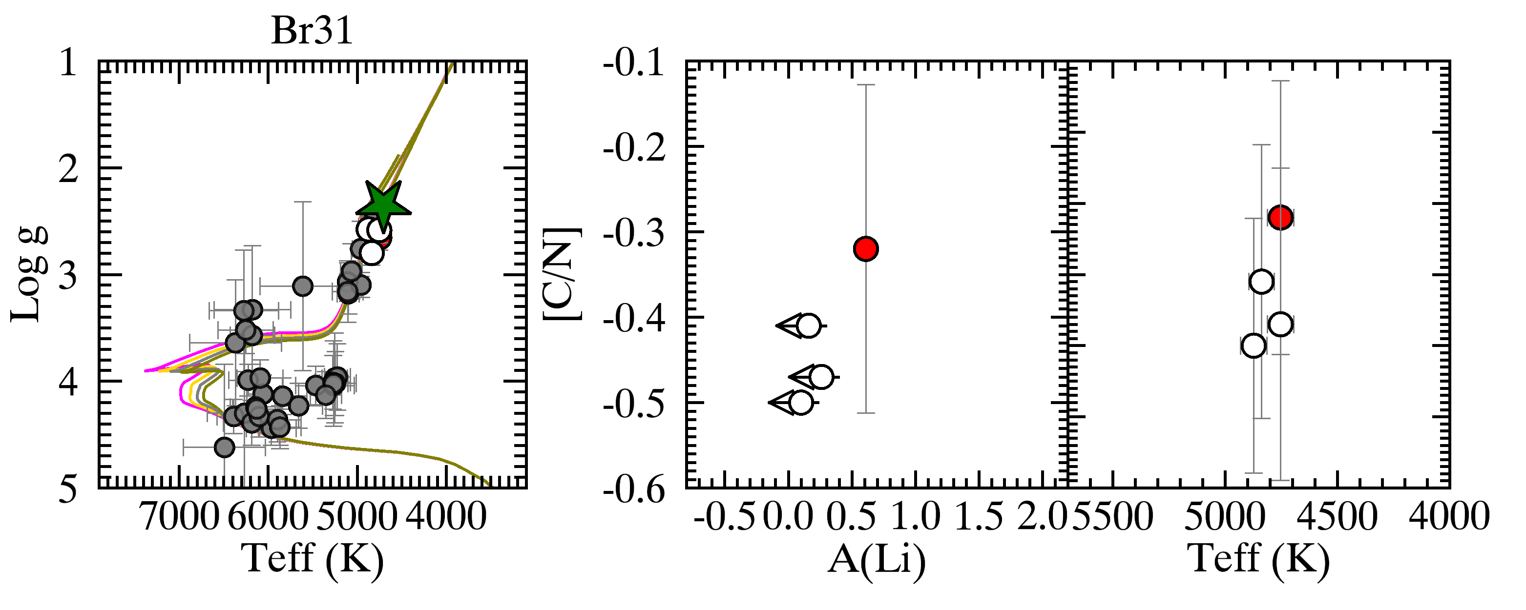
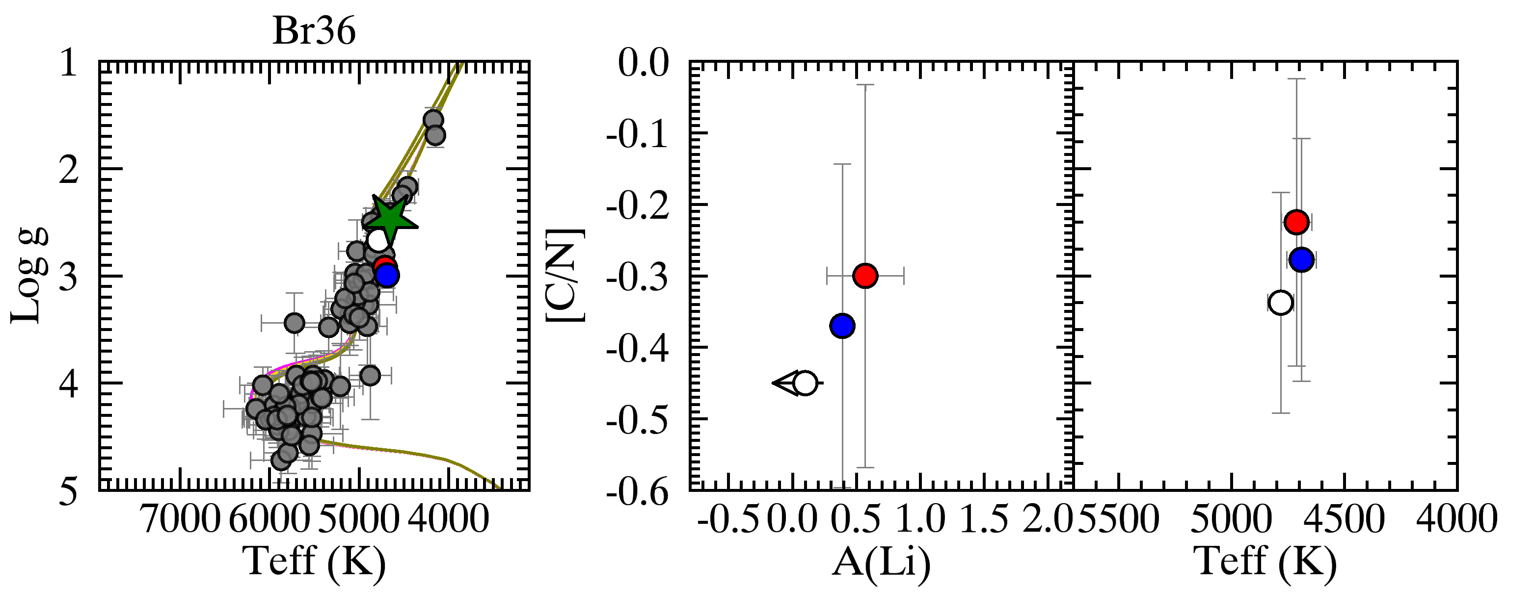
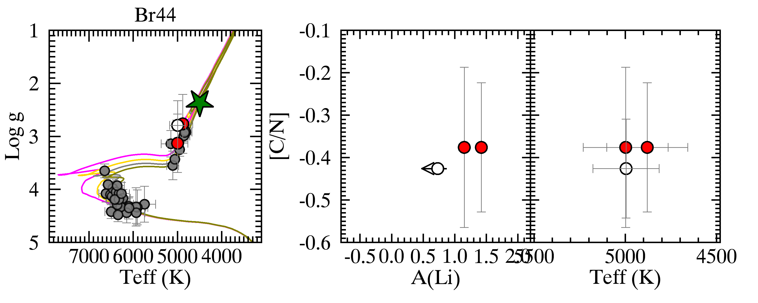
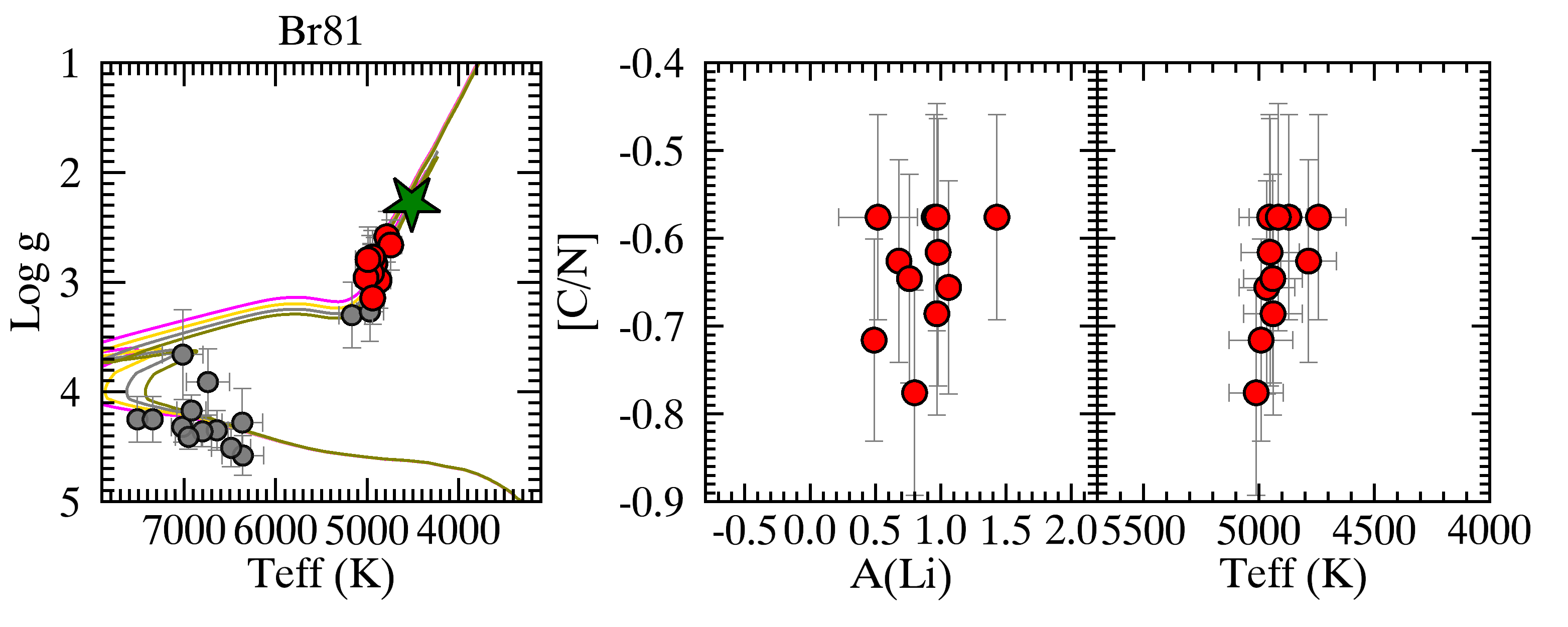
Figure 16: log $g$-T_eff diagram with PISA isochrones (left panel) and member stars beyond the FDU, A(Li) vs [C/N] (central panel), and [C/N] abundance vs T_eff (right panel) of the GES clusters. Symbols and colours as in Figure 3. The used isochrones are 2.1, 2.3, 2.5, 2.7 Gyr, 6.0, 6.5, 7.0, 7.5 Gyr, 1.1, 1.4, 1.7, 2.0 Gyr and 0.7, 0.8, 0.9, 1.0 Gyr, respectively.

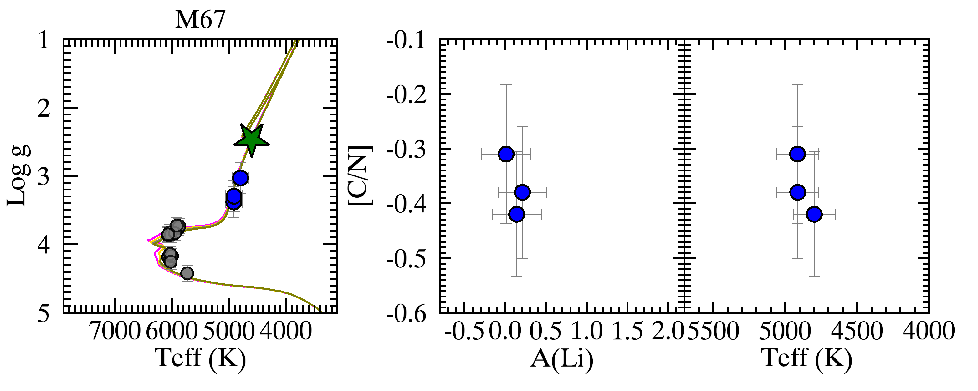
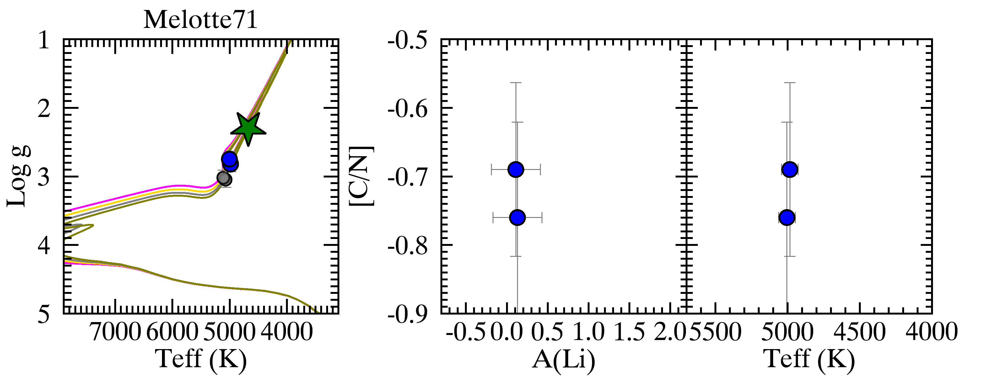
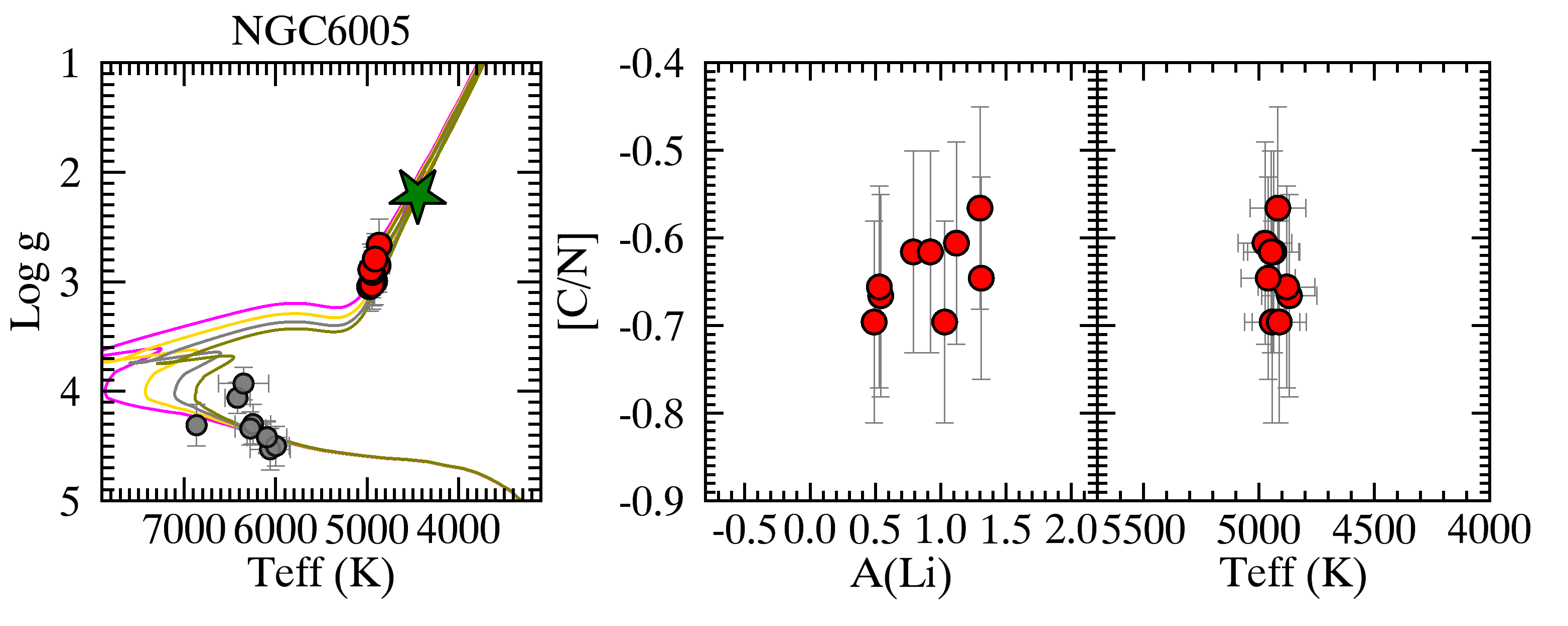
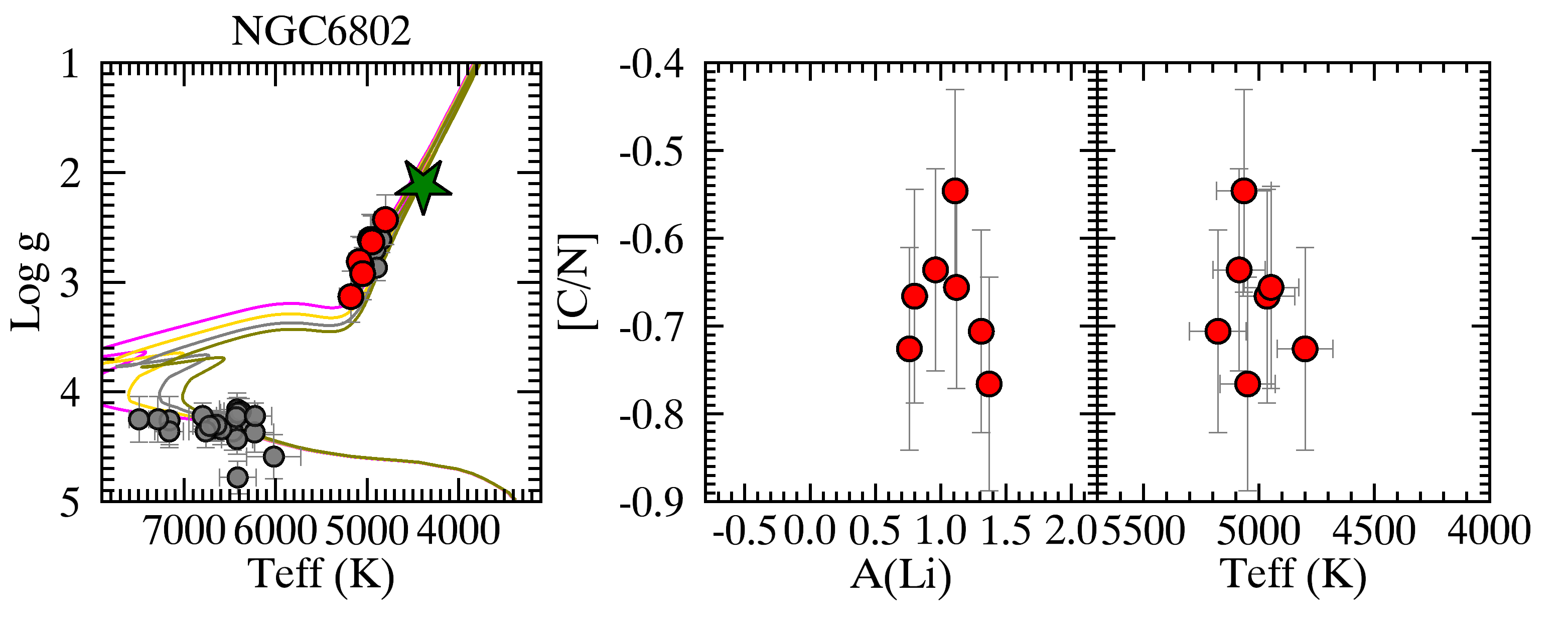
Figure 17: log $g$-T_eff diagram with PISA isochrones (left panel) and member stars beyond the FDU, A(Li) vs [C/N] (central panel), and [C/N] abundance vs T_eff (right panel) of the GES clusters. Symbols and colours as in Figure 3. The used isochrones are 3.7, 4.0, 4.3, 4.5 Gyr, 0.7, 0.8, 0.9, 1.0 Gyr, 0.8, 1.0, 1.2, 1.4 Gyr and 0.8, 1.0, 1.2, 1.4 Gyr, respectively.

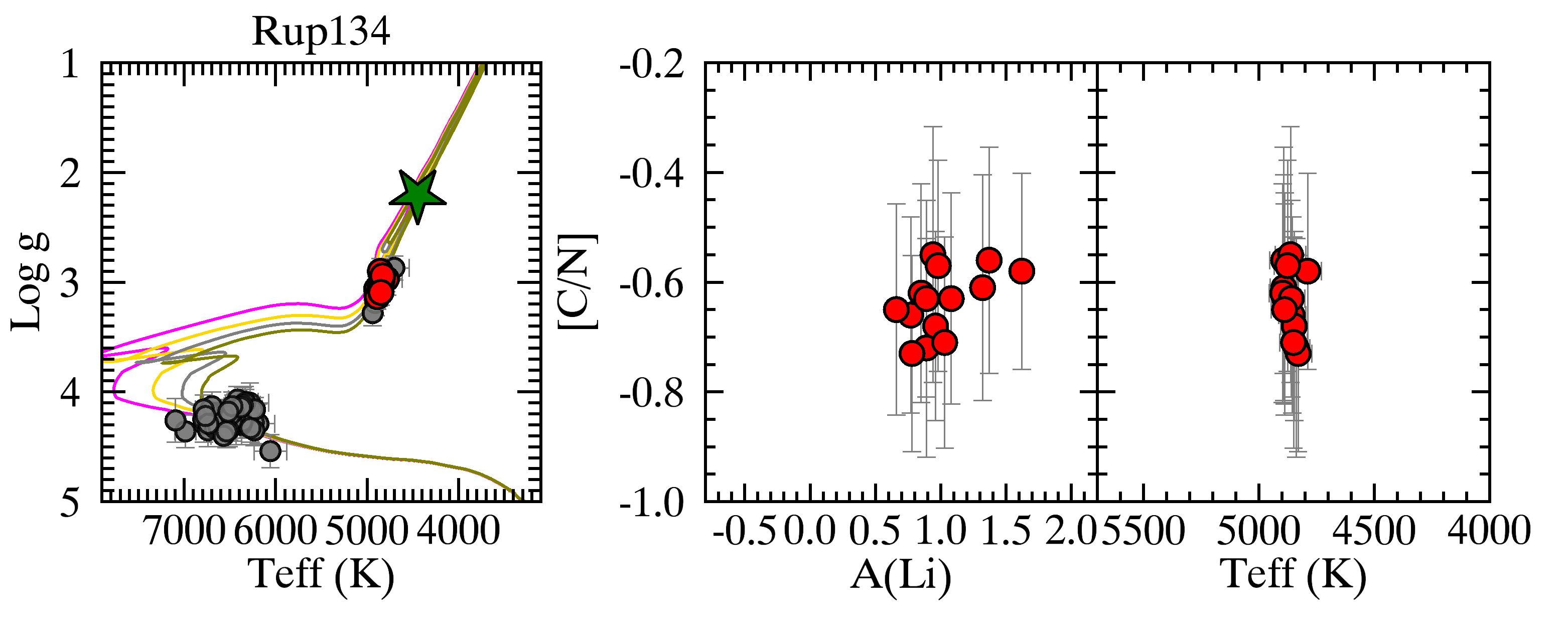
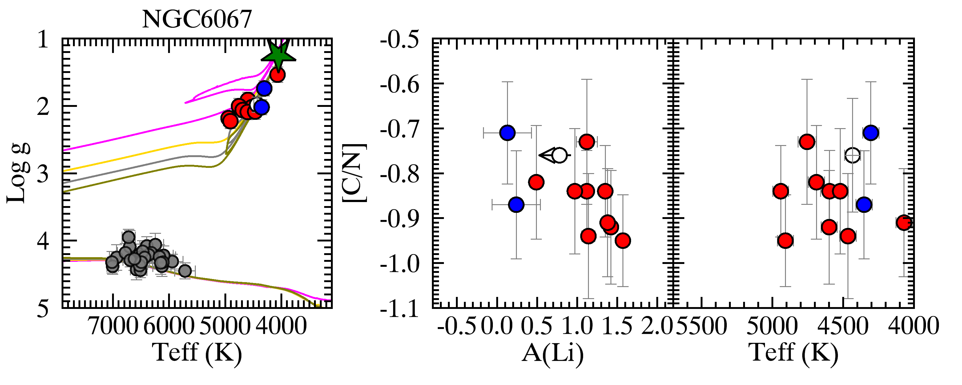
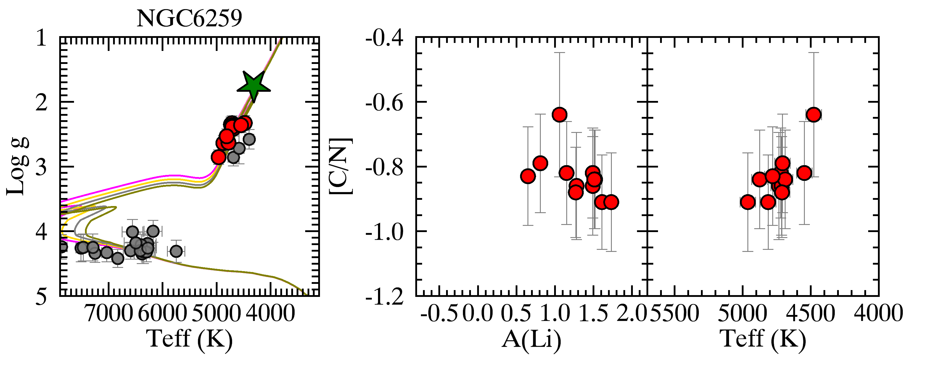
Figure 18: log $g$-T_eff diagram with PISA isochrones (left panel) and member stars beyond the FDU, A(Li) vs [C/N] (central panel), and [C/N] abundance vs T_eff (right panel) of the GES clusters. Symbols and colours as in Figure 3. The used isochrones are 0.8, 1.0, 1.2, 1.4 Gyr for the first two clusters, 0.05, 0.1, 0.2, 0.3 Gyr and 0.1, 0.2, 0.3, 0.4 Gyr, respectively.

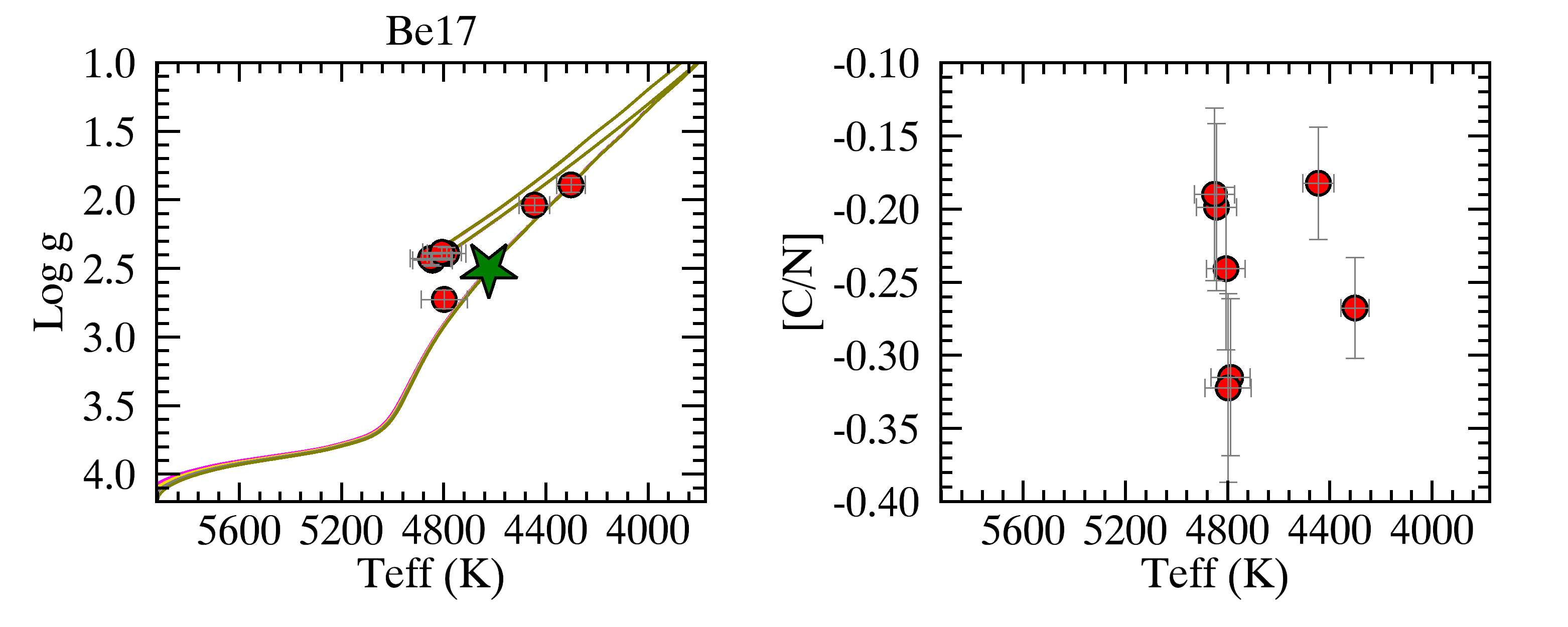
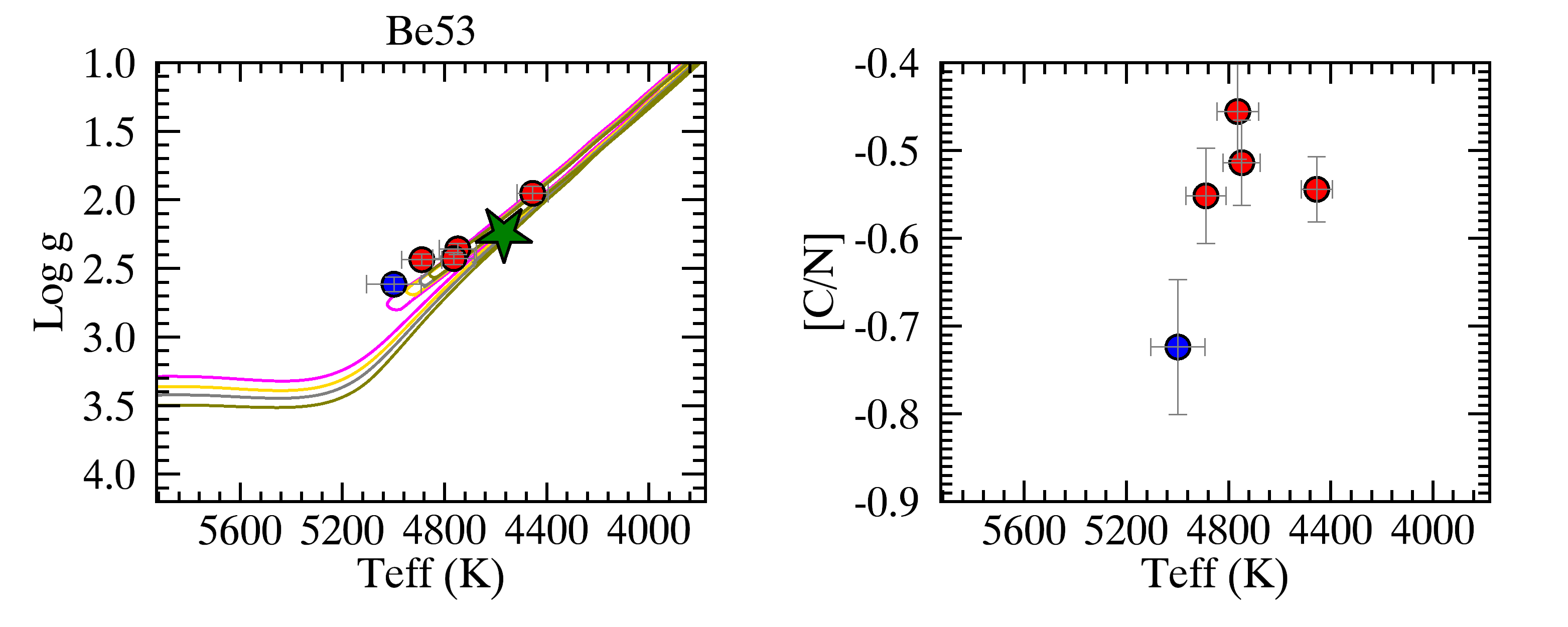
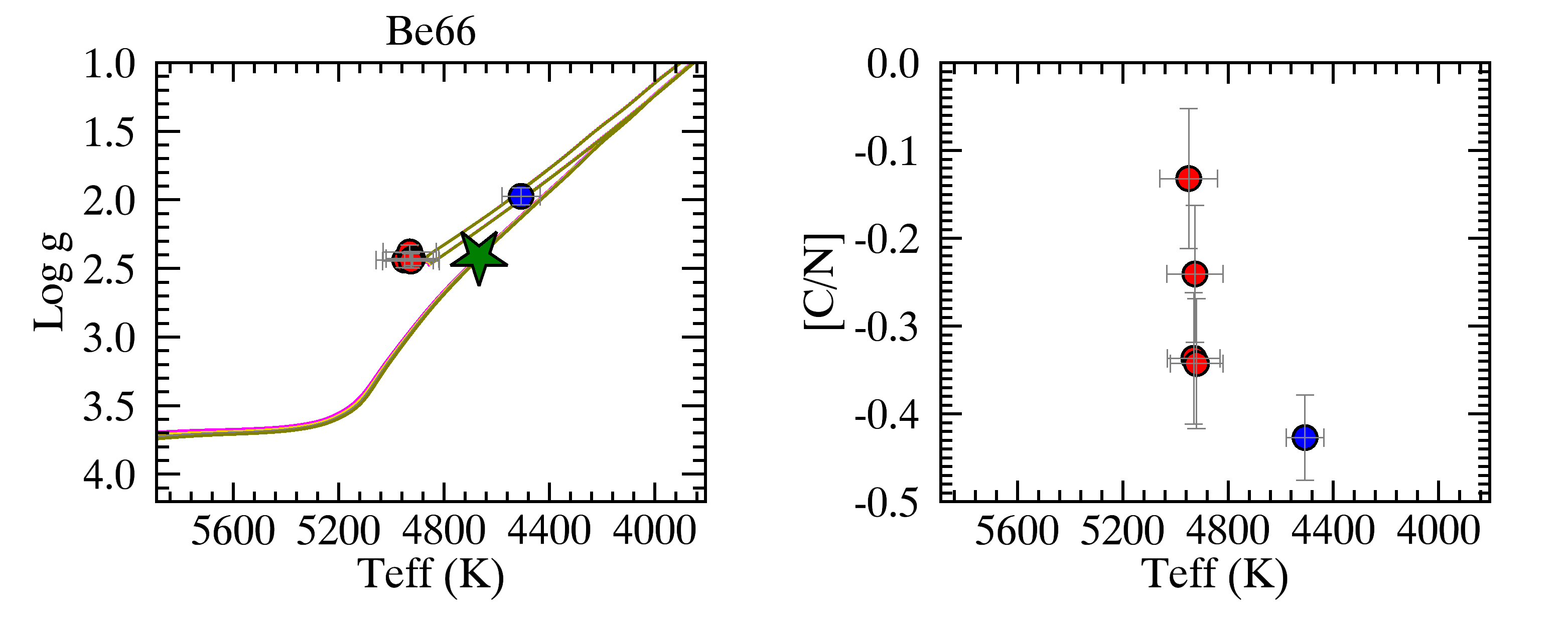
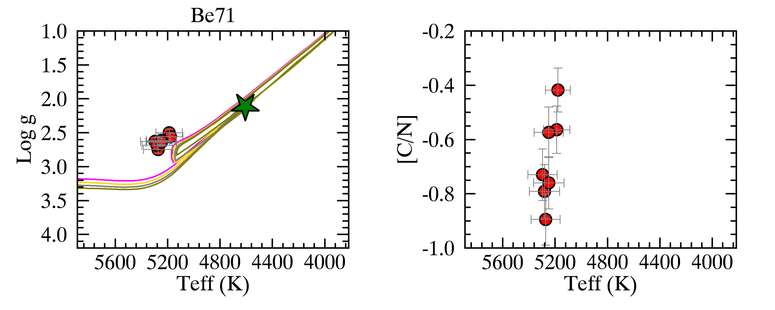
Figure 19: log $g$-T_eff diagram with PISA isochrones (left panel) and [C/N] abundance vs T_eff (right panel) of the APOGEE clusters. Symbols and colours as in Figure 4. The used isochrones are 8.8, 9.1, 9.4, 9.7 Gyr, 0.1, 1.2, 1.4, 1.7 Gyr, 3.2, 3.4, 3.6, 3.8 Gyr and 0.8, 0.9, 1.0, 1.1 Gyr, respectively.

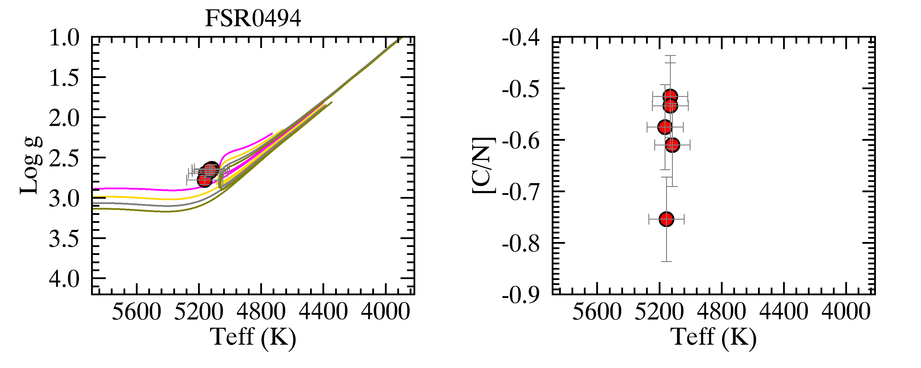
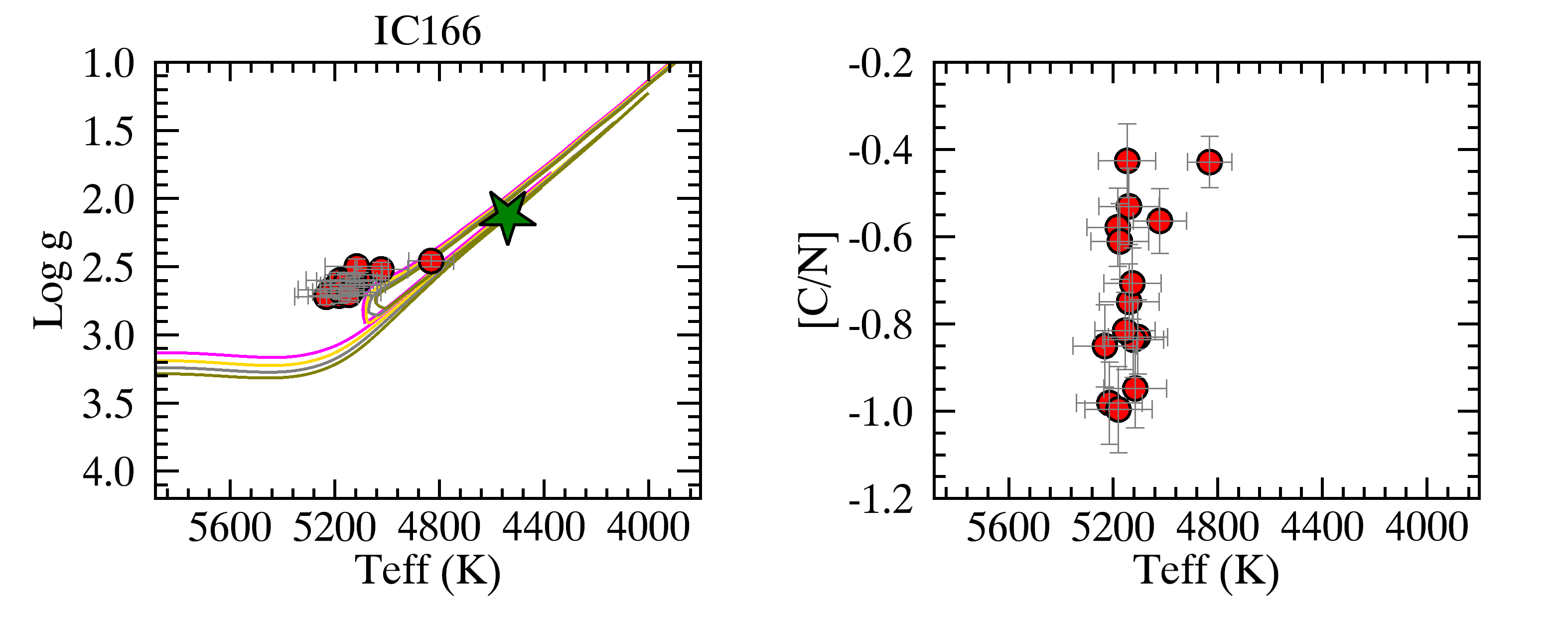
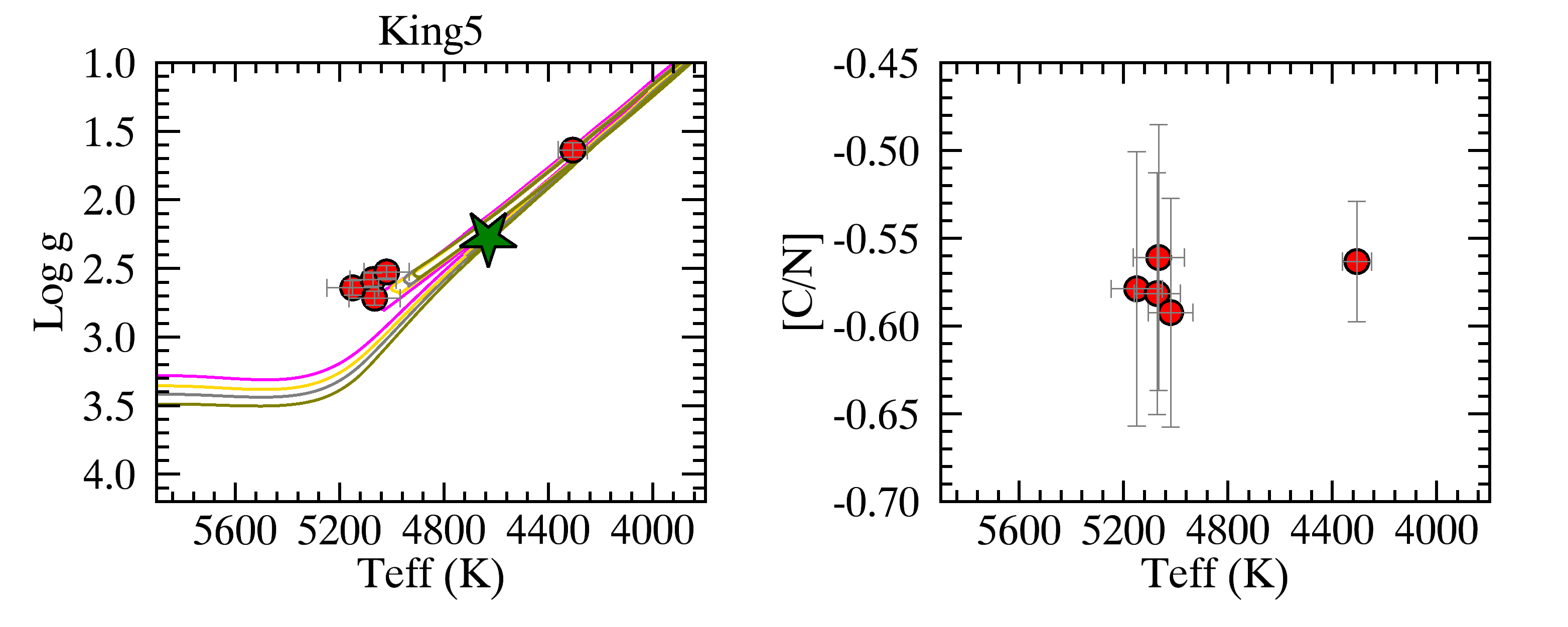
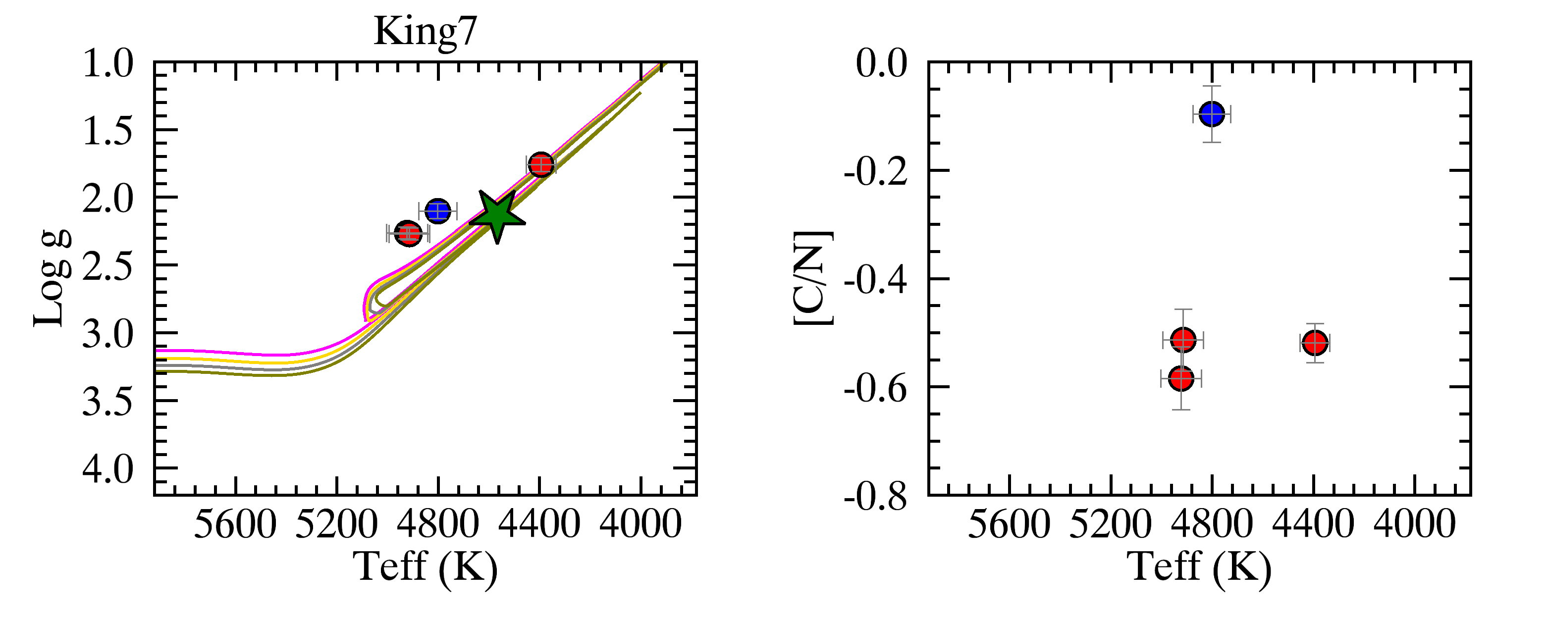
Figure 20: log $g$-T_eff diagram with PISA isochrones (left panel) and [C/N] abundance vs T_eff (right panel) of the APOGEE clusters. Symbols and colours as in Figure 4. The used isochrones are 0.4, 0.5, 0.6, 0.7 Gyr, 0.6, 0.8, 1.0, 1.2 Gyr, 1.0, 1.2, 1.4, 1.7 Gyr and 0.4, 0.5, 0.6, 0.7 Gyr, respectively.

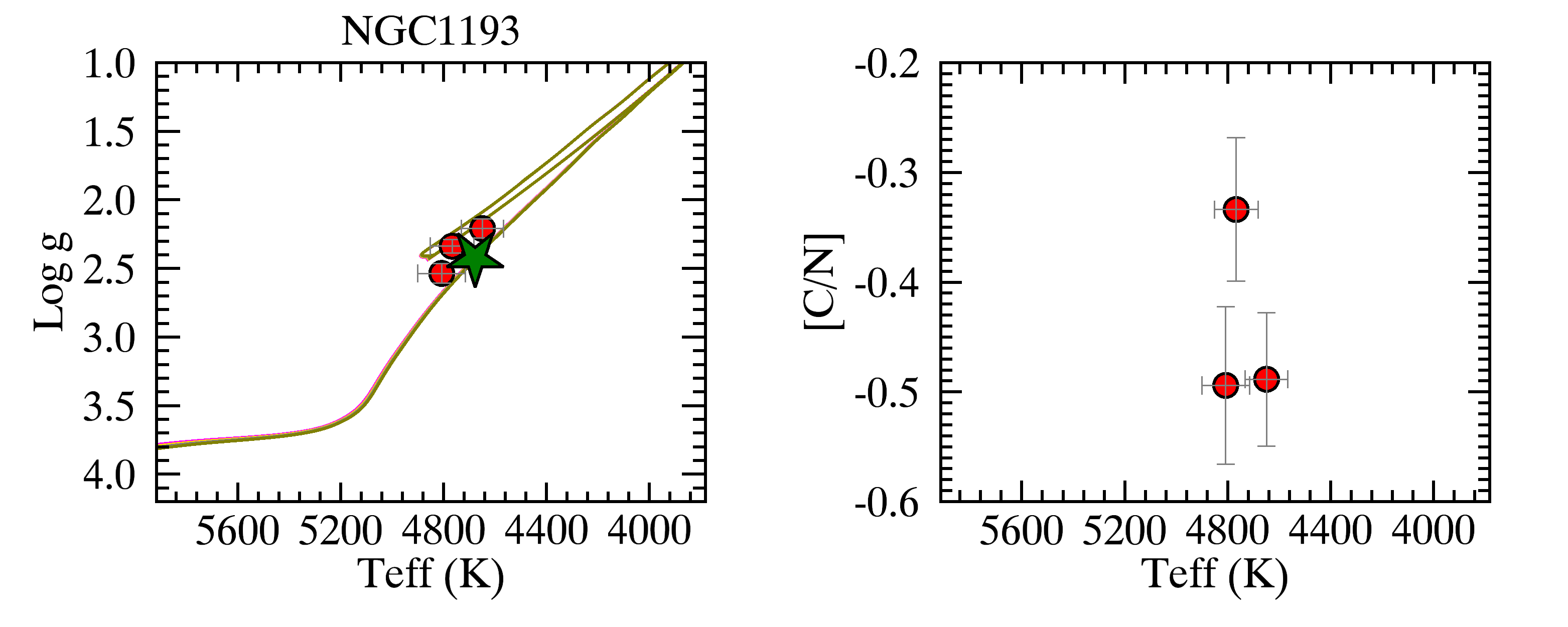
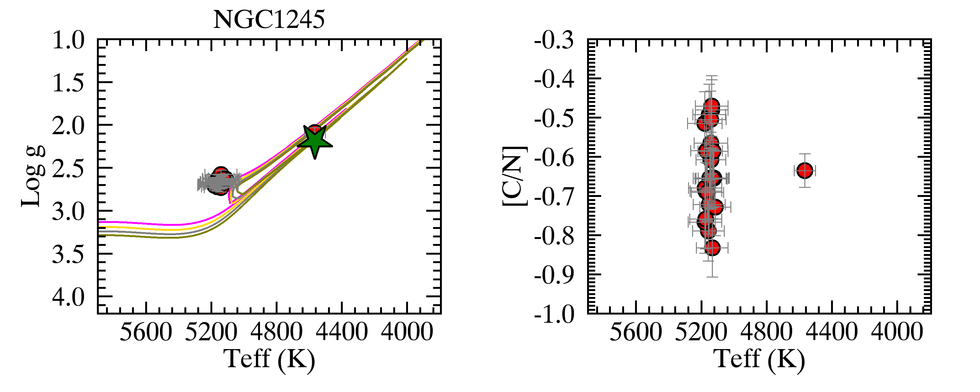
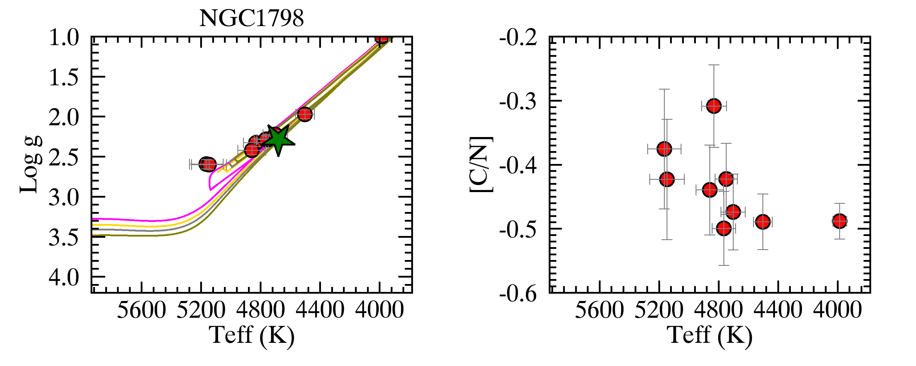
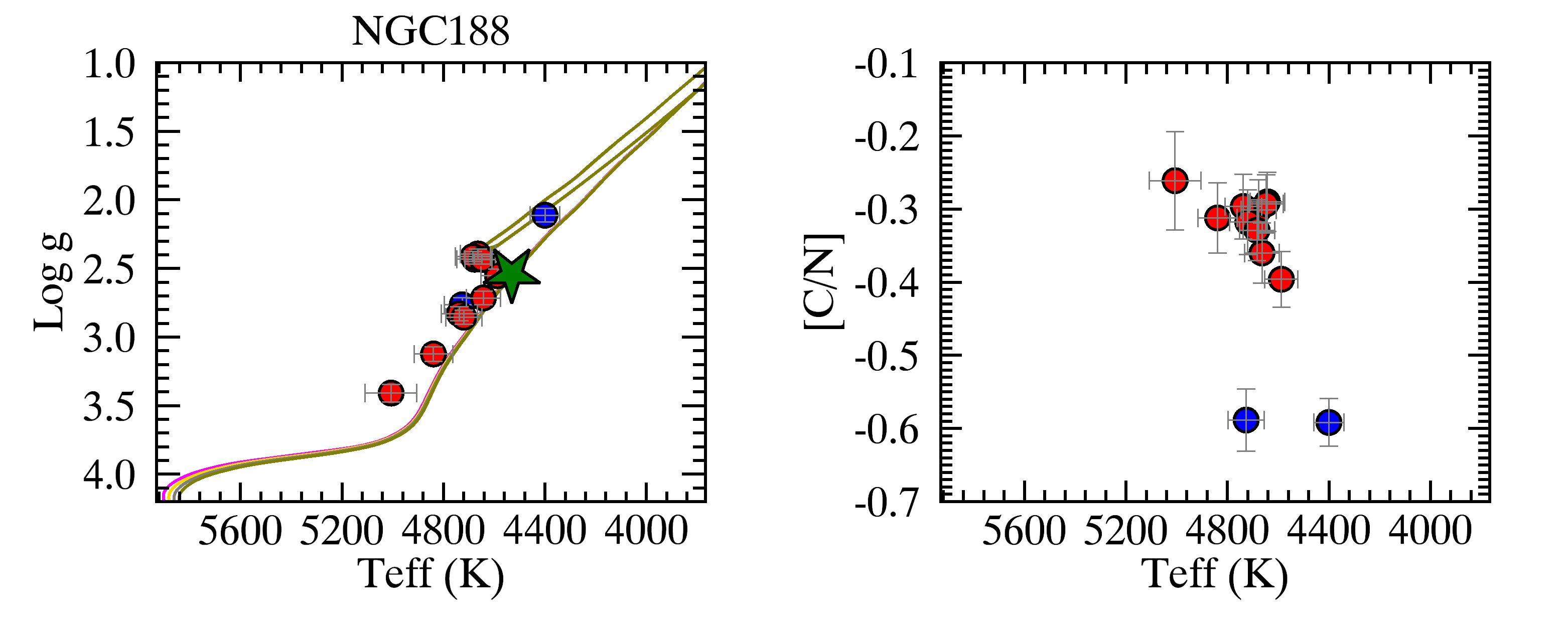
Figure 21: log $g$-T_eff diagram with PISA isochrones (left panel) and [C/N] abundance vs T_eff (right panel) of the APOGEE clusters. Symbols and colours as in Figure 4. The used isochrones are 4.6, 4.8, 5.0, 5.2 Gyr, 0.7, 0.8, 0.9, 1.0 Gyr, 1.0, 1.2, 1.4, 1.7 Gyr and 7.3, 7.6, 7.9, 8.2 Gyr, respectively.

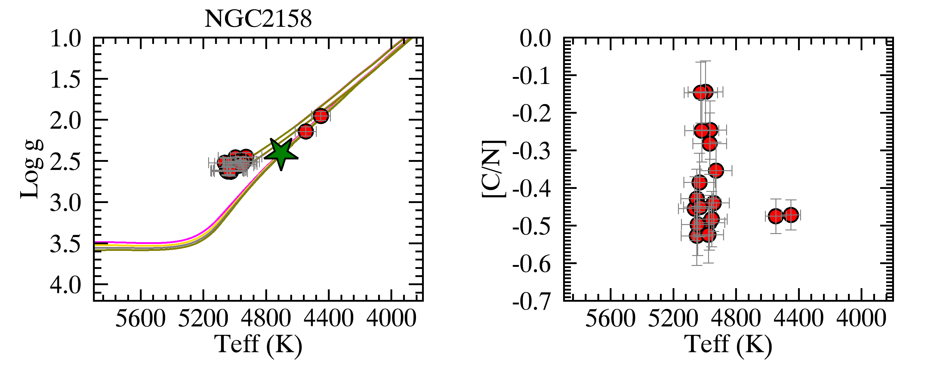
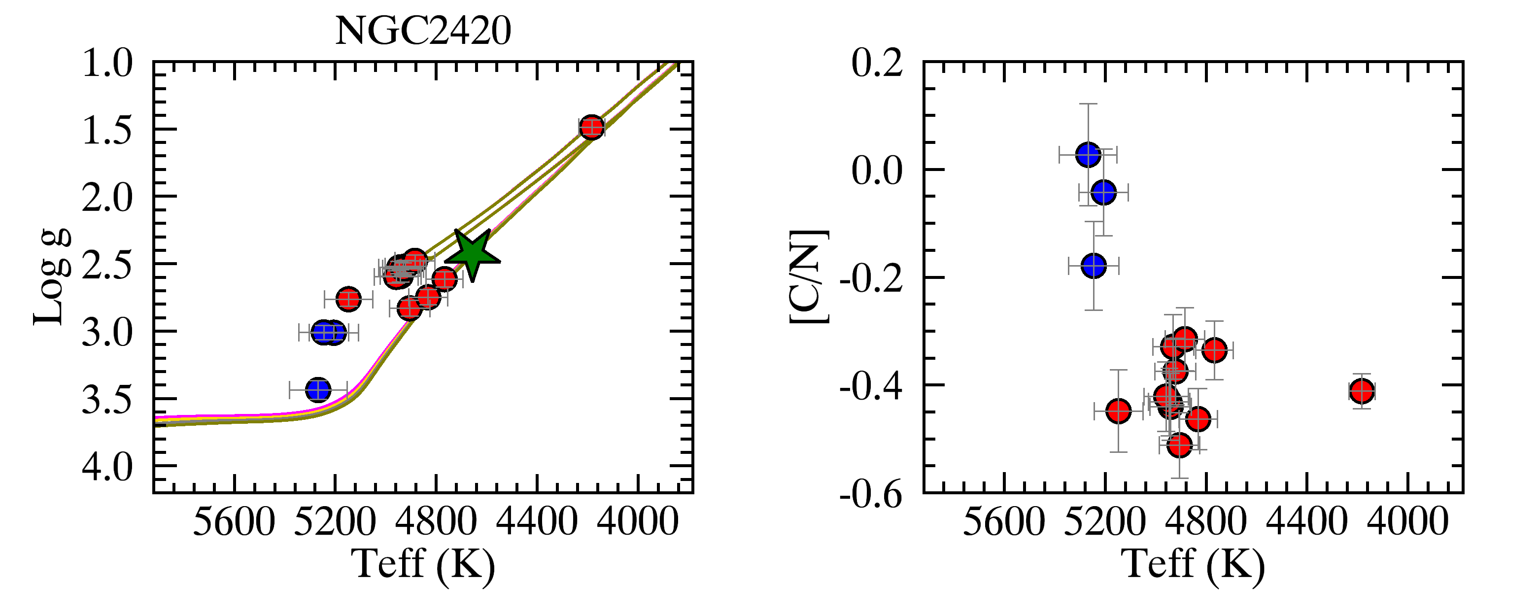
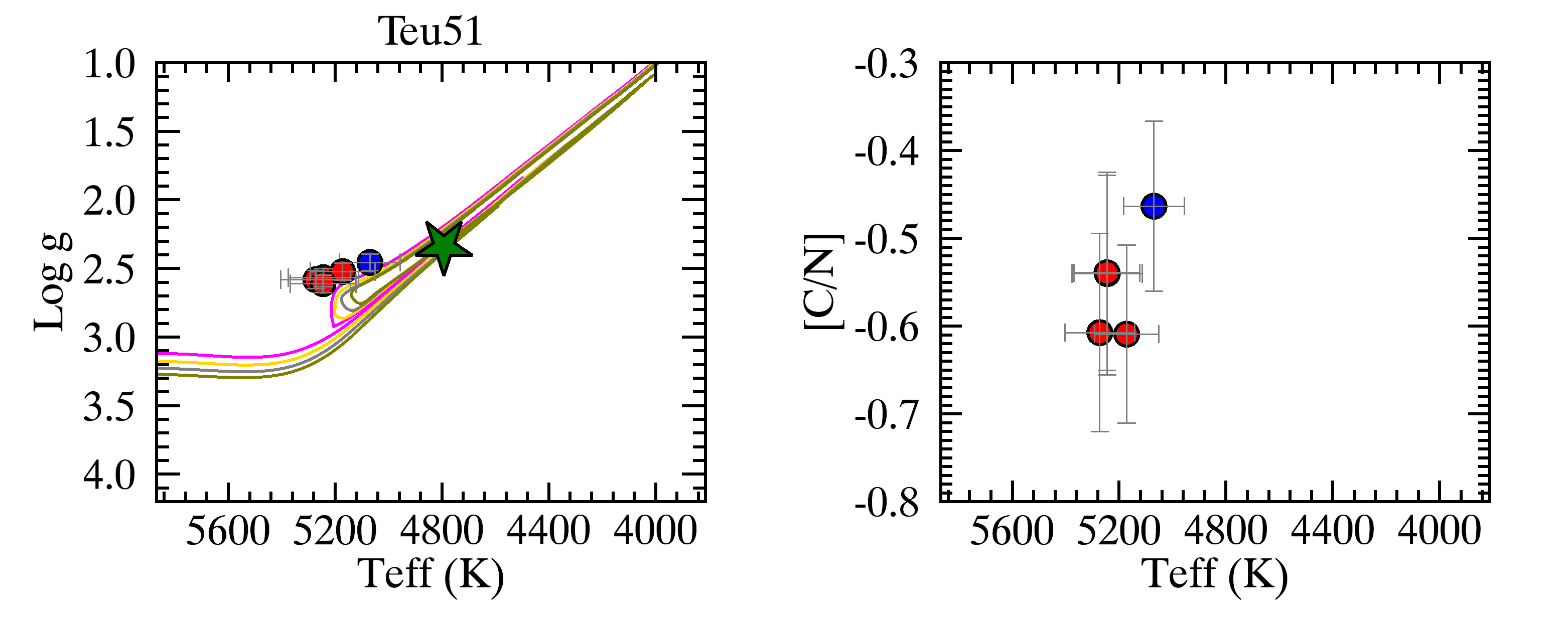
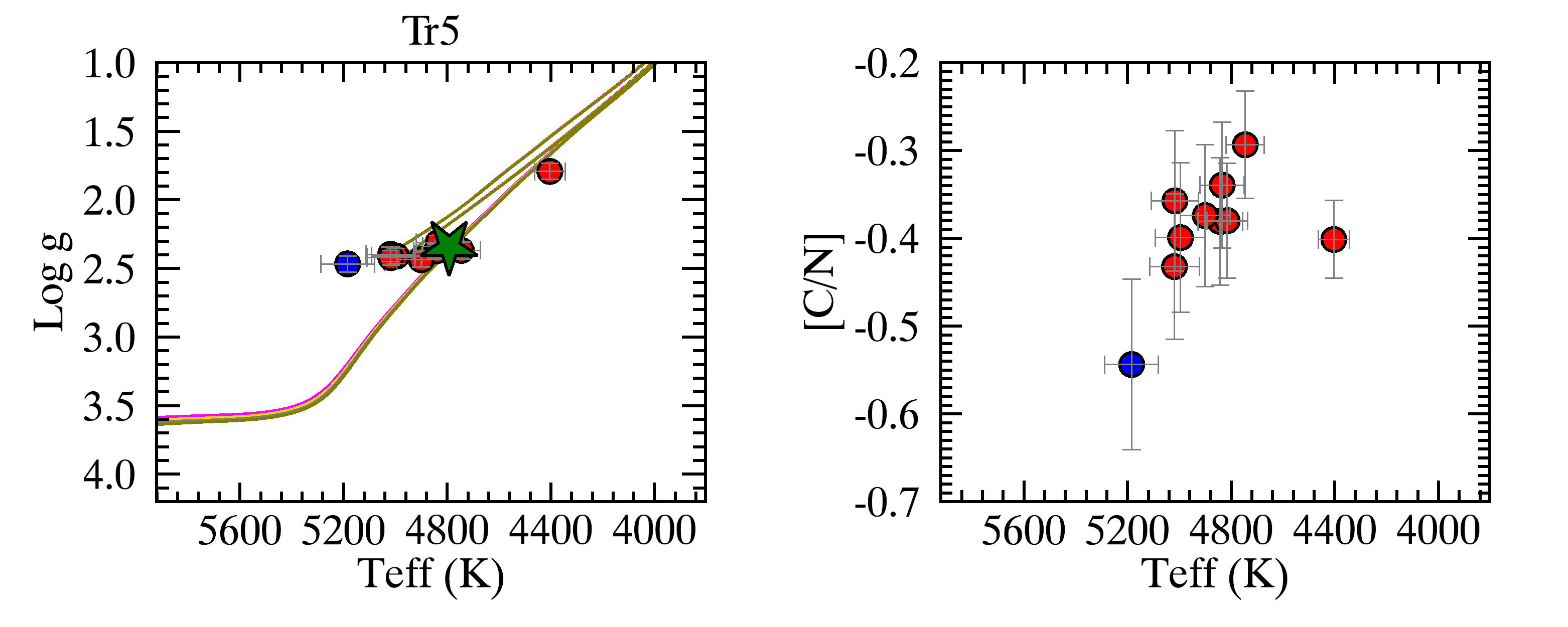
Figure 22: log $g$-T_eff diagram with PISA isochrones (left panel) and [C/N] abundance vs T_eff (right panel) of the APOGEE clusters. Symbols and colours as in Figure 4. The used isochrones are 1.7, 1.9, 2.1, 2.3 Gyr, 2.6, 2.8, 3.0, 3.2 Gyr, 0.7, 0.8, 0.9, 1.0 Gyr and 2.6, 2.8, 3.0, 3.2 Gyr, respectively.

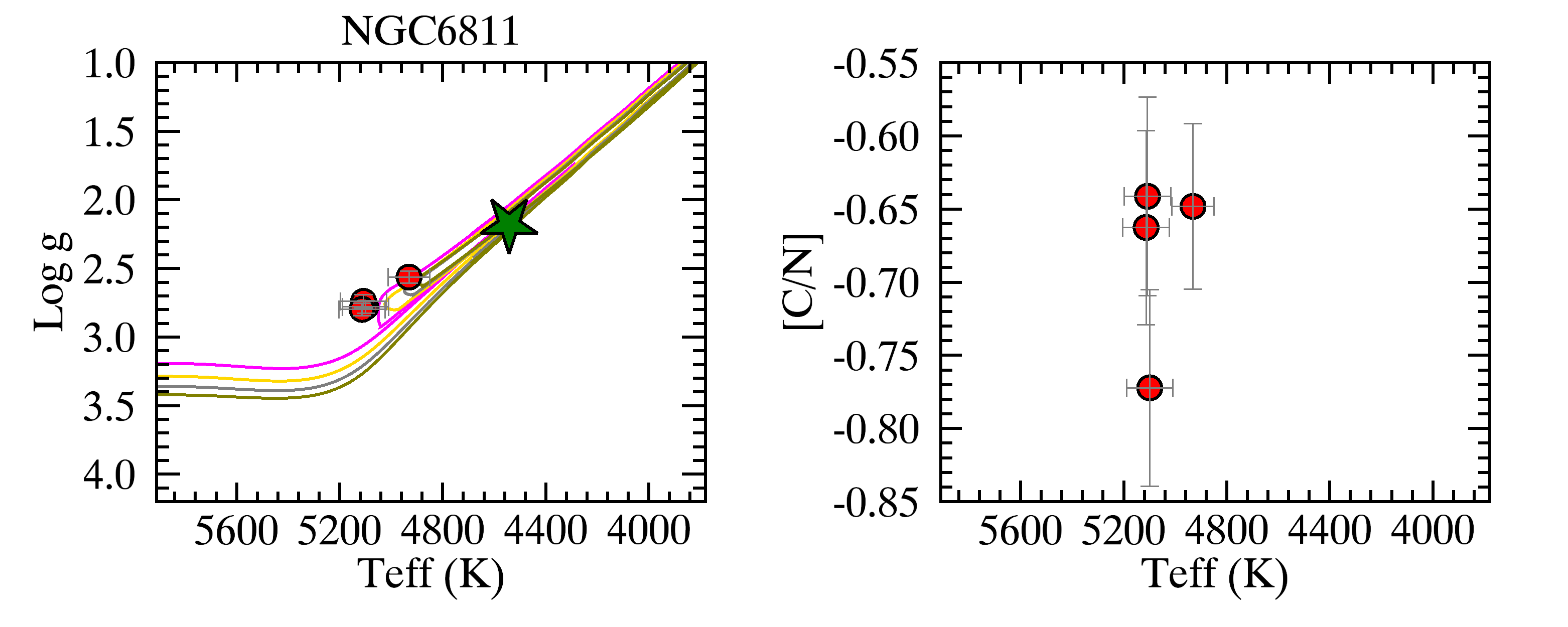
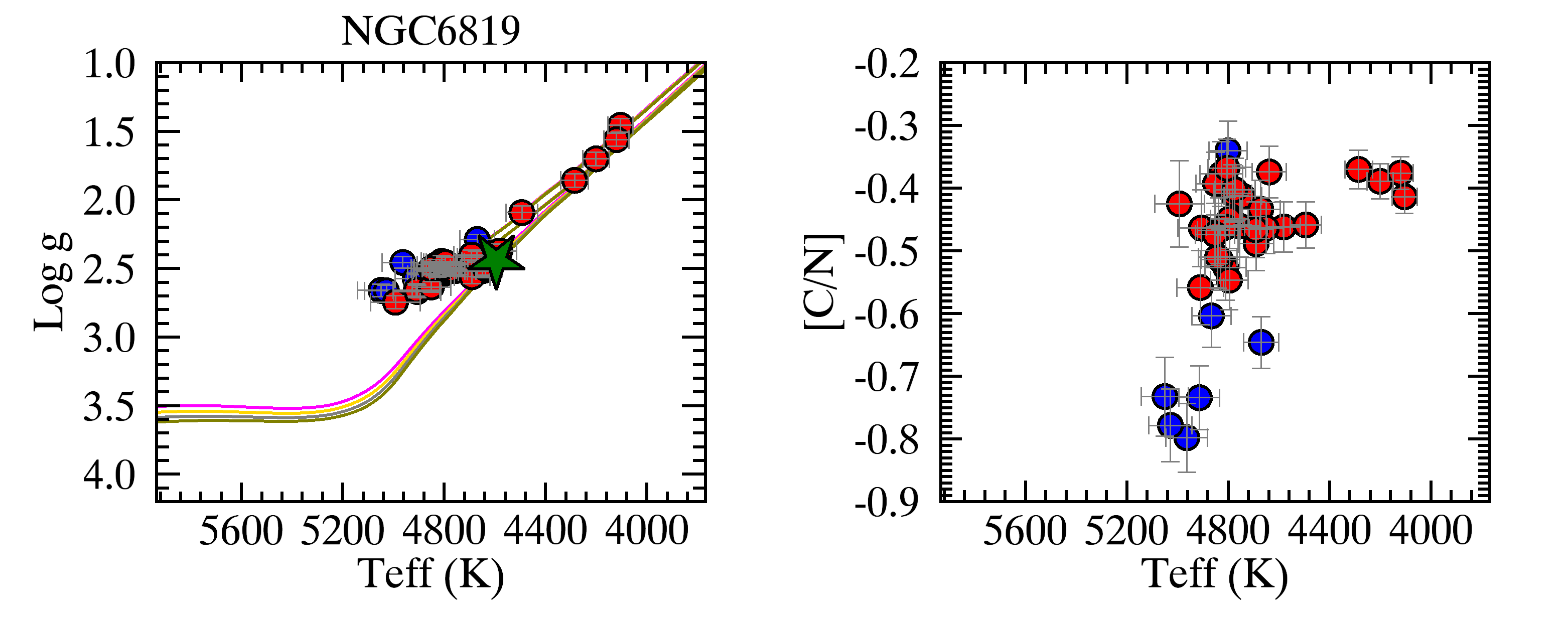
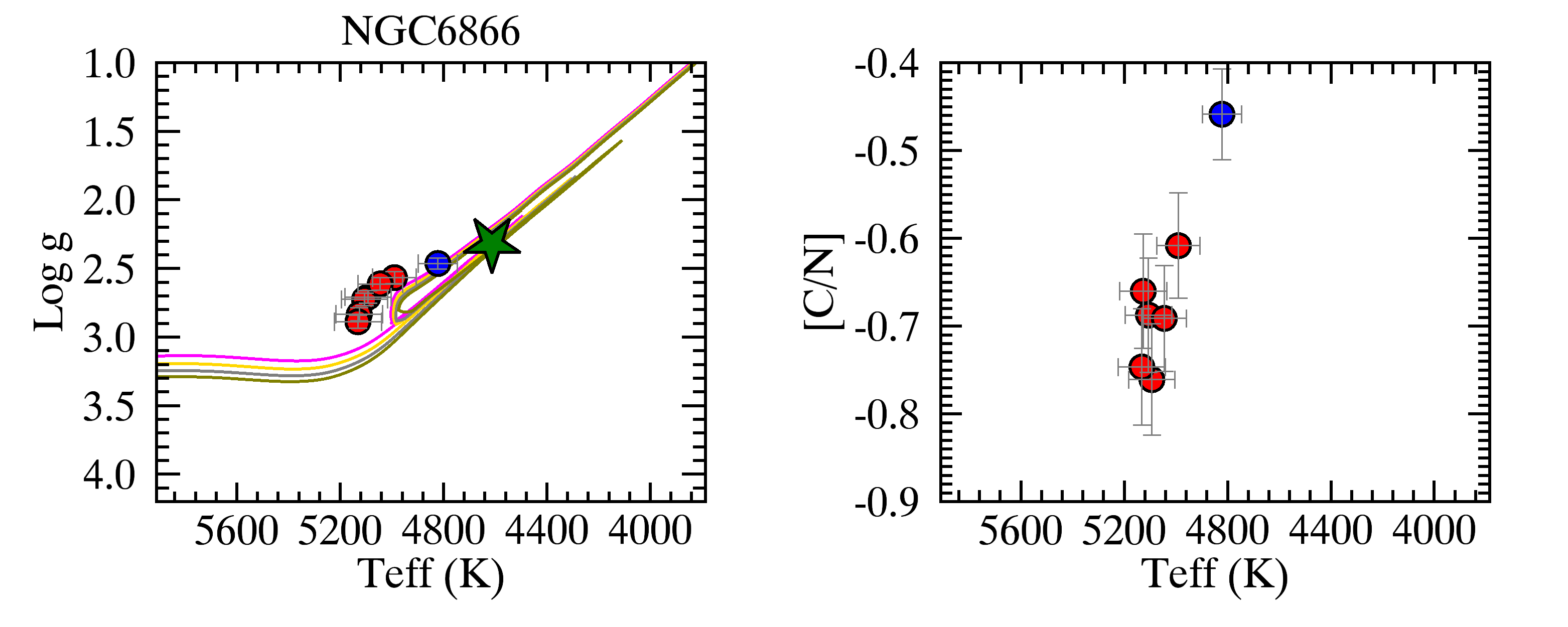
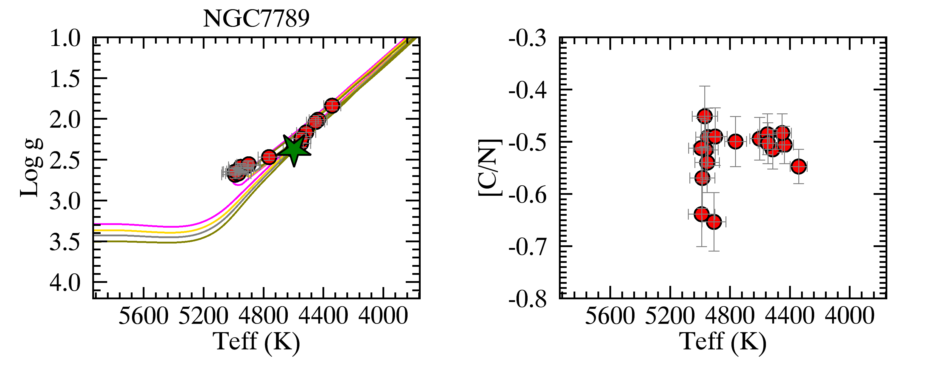
Figure 23: log $g$-T_eff diagram with PISA isochrones (left panel) and [C/N] abundance vs T_eff (right panel) of the APOGEE clusters. Symbols and colours as in Figure 4. The used isochrones are 0.8, 1.0, 1.2, 1.4 Gyr, 1.7, 1.9, 2.1, 2.3 Gyr, 0.7, 0.8, 0.9, 1.0 Gyr and 1.0, 1.2, 1.4, 1.7 Gyr, respectively.

For the open clusters in the GES sample we also add stars observed with GIRAFFE, mainly in the main sequence for a better characterisation of the cluster sequence. The agreement between the literature ages and metallicities and the corresponding isochrones is remarkably good, since most of them were recently re-determined by the Gaia-ESA consortium in a homogeneous way (see, e.g., Donati et al. 2014; Friel et al. 2014; Jacobson et al. 2016a; Magrini et al. 2017; Overbeek et al. 2017; Tang et al. 2017; Randich et al. 2018). For the APOGEE sample, most of the clusters are in agreement with the PISA isochrones computed with the literature ages and metallicities. We only redetermine the age of FSR0494, for which the PISA isochrone for the age given by Kharchenko et al. (2013) is inconsistent with the present data. The new age is listed in Table 2. In the left panels of Fig. 3 in Sec. 3 and in Figs. 16, 17, 18 in the Appendix, we show the log $g$-T_eff diagrams of member stars of each GES cluster with the corresponding PISA isochrones. Instead, the colour-magnitude diagrams of NGC 4815, NGC 6705 and Trumpler 20 are shown in Tautvaišienė et al. (2015). In Fig 4 and in Figs. 19, 20, 21, 22, 23, (left panels) the log $g$-T_eff diagrams of APOGEE member stars and the PISA isochrones are shown.

3 The selection criteria

To build-up a relationship between the cluster [C/N] abundance ratios and their ages, it is necessary to select member stars in the red-giant branch (RGB) that have already modified their carbon and nitrogen surface abundances, passing through the FDU event.

3.1 The selection of red giant stars beyond the FDU

We derive a quantitative criterion to select among the member stars of our sample open clusters those which have passed the FDU. To identify the location in the log $g$-T_eff diagram at which the FDU occurs for clusters of different ages and metallicities, in particularly the surface gravity log $g$, we use the same set of isochrones employed to check cluster ages. We consider isochrones in the age and metallicity ranges of our clusters, i.e., with [Fe/H] from $-0.4$ to $+0.4$ dex and with ages from 0.1 to 10 Gyr. For these isochrones, we obtain the surface abundances of N and C.

The surface gravity that corresponds to the FDU has been identified by selecting a proper value where the [C/N] starts to monotonically decrease. Indeed, during the FDU the surface [C/N] abundance progressively decreases as surface convection reaches deeper and deeper regions inside the star. We tried two different approaches: 1) the point where [C/N] starts to monotonically decrease or 2) the point where the derivative $d[C/N]/d\log g$ is maximum. We tested these two criteria on clusters with ages larger than 2 Gyr finding that the difference in the location of the FDU in the log $g$ plane is quite negligible for our purposes (about 0.1 dex).

On the other hand, the second method (the point where $d[C/N]/d\log g$ is maximum) is not suitable for clusters with ages below 500 Myr/1 Gyr. The reason is that for such ages, the extension of the convective envelope and consequently the surface [C/N] abundance changes slowly with log $g$, causing a significant difference between the $\log g$ at FDU estimated using the two methods.

Figure 1 shows, as an example, the variation of [C/N] vs $\log g$ for isochrones of 200 Myr and 2 Gyr (for solar metallicity). For the 2 Gyr case the interval of $\log g$ where [C/N] starts/stops decreasing is $\Delta\log g\approx 0.3$-0.4 dex, while for young clusters the interval is larger, of about 0.6-0.7 dex. The maximum of the derivative $d[C/N]/d\log g$ corresponds to about the median point of the interval. Given the large interval of $\log g$ during the giant branch in young clusters, the adoption of the maximum derivative underestimates $\log g$ at the FDU by about 0.3 dex with respect to the alternative criterion. For this reason, we decided to use the first approach and, therefore, identify the $\log g$ FDU as the point where [C/N] starts to monotonically decrease, in all the analyzed clusters.

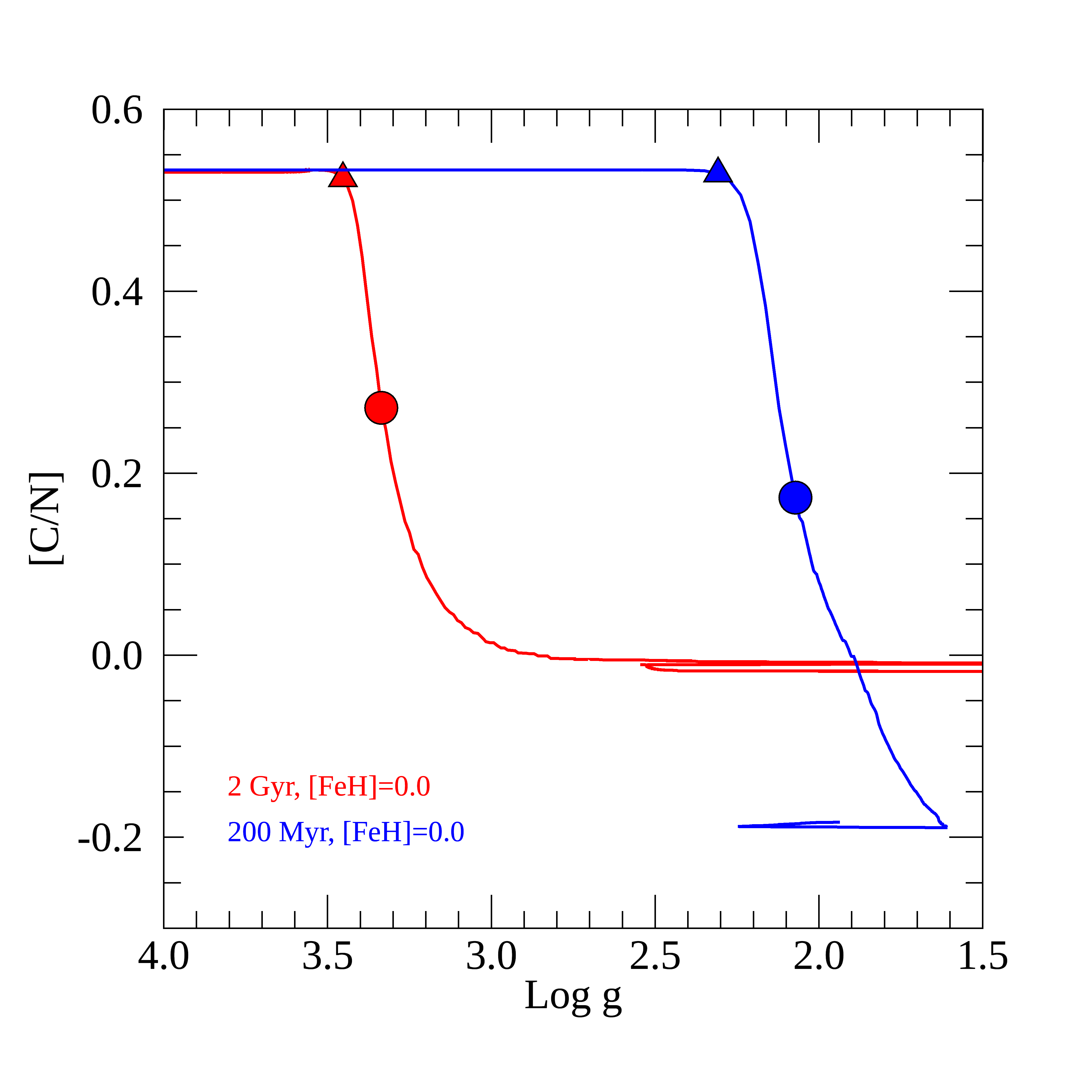
Figure 1: [C/N] vs log $g$ of 200 Myr (red line) and 2 Gyr (blue line) [Fe/H]=$0.0$ dex PISA isochrones. The triangle represents the point where [C/N] starts to monotonically decrease, while the circle represents the point where the derivative $d[C/N]/d\log g$ is maximum.

For each cluster in both GES and APOGEE samples, the values of log $g$ corresponding to the FDU are shown in Table  3. To estimate the uncertainties in log $g$ at which the FDU happens, we consider how the uncertainties on the age and metallicity reflect on the position of the FDU in the age vs. log $g$(FDU) plane, as shown in Figure 2. At younger ages, the uncertainty on the location of the FDU is mainly due to the uncertainties on the age. For the youngest clusters, with age $<$ 1 Gyr, the uncertainty in the determination of the log $g$ of the FDU can be very large, since the log $g$ range in which the FDU occurs is wide ($\sim$1 dex in log $g$). Typical uncertainties of clusters with ages of about 1 Gyr ranges from 0.1 to 0.3 Gyr (see Tables 1 and 2), thus implying an uncertainty in the determination of the log $g$ of the FDU of $\sim$0.05 dex. For the oldest clusters, the main variation in the FDU position is related to the uncertainty in metallicity: from 2 to 9 Gyr, a variation of [Fe/H] of $\pm$0.15 dex implies a change in the FDU log $g$ from 0.05 to 0.1 dex, respectively. To select stars which have passed the FDU, we take into account both the uncertainties on the estimation of the theoretical position of the FDU and on the derived spectroscopic gravities. These uncertainties are added to FDU log $g$ in order to have a lower limit in the selection of stars beyond the first dredge-up.

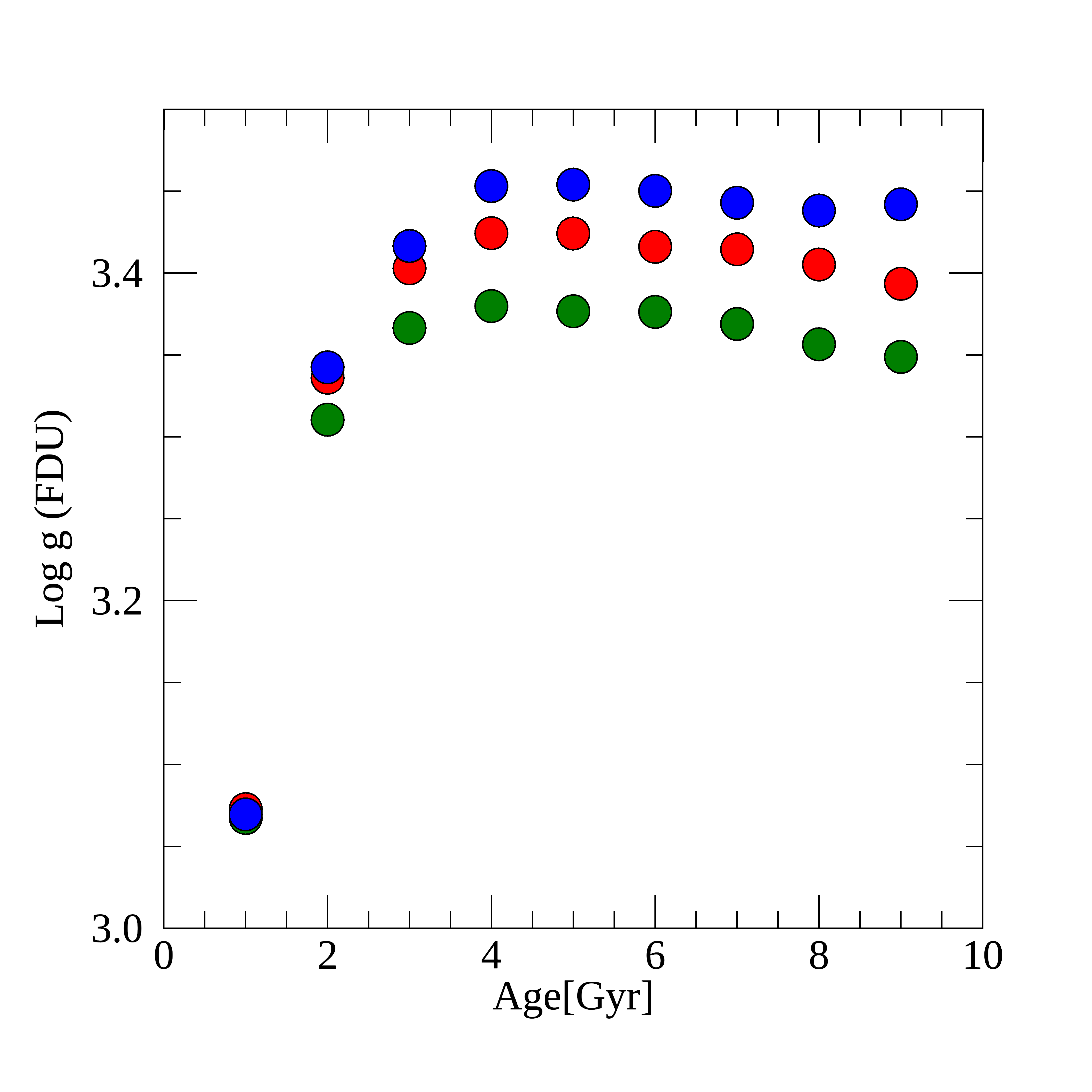
Figure 2: Theoretical log $g$ at the FDU as a function of age and metallicity. Three different colours indicate three different metallicities: [Fe/H]=0 (red), [Fe/H]=$-$0.15 (green) and [Fe/H]=+0.15 (blue).

Table 3: Surface gravity, log $g$, at FDU for the open clusters in the GES and APOGEE samples.

Open Clusters	log $g$ at FDU
	(dex)
GES clusters
Berkeley 31	3.5
Berkeley 36	3.5
Berkeley 44	3.4
Berkeley 81	3.1
Melotte 71	3.1
NGC 2243	3.5
NGC 6005	3.3
NGC 6067	2.1
NGC 6259	2.4
NGC 6802	3.2
Rup134	3.2
Pismis 18	3.3
Trumpler 23	3.1
APOGEE clusters
Berkeley 17	3.5
Berkeley 53	3.3
Berkeley 66	3.5
Berkeley 71	3.2
FSR0494	2.8
IC166	3.2
King 5	3.3
King 7	3.0
NGC 1193	3.5
NGC 1245	3.2
NGC 1798	3.3
NGC 188	3.6
NGC 2158	3.4
NGC 2420	3.5
NGC 6791	3.6
NGC 6811	3.2
NGC 6819	3.4
NGC 6866	3.1
Teutsch 51	3.1
Trumpler 5	3.4
NGC 7789	3.4
GES and APOGEE clusters
M67	3.4
NGC 6705	2.6

3.2 C and N variations beyond the FDU: the effect of extra-mixing

Selecting stars which have passed the FDU defines indeed a broad class of giant stars: lower-RGB stars, i.e. stars just after the phase of sub-giant, at the beginning of the RGB; stars in the red clump (RC), and stars in the upper-RGB. After the FDU, star evolves along the RGB where more mixing can occur, further decreasing the C/N ratio (see, for instance Gratton et al. 2000; Martell et al. 2008) due to non-canonical mixing possibly driven by thermohaline mechanisms (Lagarde et al. 2012). These effects are mainly expected along the upper-RGB, after the RGB bump phase, and they are more important at low metallicity and for low-mass stars (see the lower panel of Fig.1 of Masseron & Gilmore 2015; Shetrone et al. 2019). On the other hand, at solar metallicity and for massive stars, the effect is quite small and almost negligible compared to the precision of measured C/N, unless other non-canonical extra-mixing processes modified them in specific stars. Masseron et al. (2017) confirmed the universality of extra-mixing along the upper part of the RGB for low mass stars. They found a N depletion between the RGB tip and the He-burning phase/clump evolutionary stages, likely due to the mixing with the outer envelope during the He flash. This effect is particularly appreciable and strong at low metallicity, while at solar metallicity RGB and RC stars present similar N abundances (Shetrone et al. 2019).

Observational evidences of mixing processes happening during the RGB-bump phase have been the detection of a further depletion of Li abundance along the RGB in globular clusters (e.g., Lind et al. 2009; Mucciarelli et al. 2011). During the bump, indeed, the thermohaline convection is expected to be more efficient and to rapidly transport surface Li in the internal hotter regions where it is destroyed. The same mechanism can modify C and N abundances.

Open clusters usually do not reach very low metallicities and thus are not expected to show strong extra mixing. Nevertheless, thanks to the GES data, we can check cluster by cluster whether this extra mixing occur by looking at Li abundance, A(Li)=$\log$(Li/H), and [C/N]. Then we can safely exclude the stars with strong extra-mixing with lower [C/N] and which would affect our age determination. In our sample, the lowest metallicities are those of Br 31 ([Fe/H]=$-$0.27$\pm$0.06) and NGC 2243 ([Fe/H]=$-$0.38$\pm$0.04) in the GES sample and of Trumpler 5 ([Fe/H]=$-$0.40$\pm$0.01) and Teutsch 51 ([Fe/H]=$-$0.28$\pm$0.03) in the APOGEE sample. As shown in Fig.1 of Masseron & Gilmore (2015), [C/N] from lower RGB to RC should be unchanged at solar metallicity, while it is expected to be modified in the upper-RGB, but at lower metallicity. Although from a theoretical point of view, we do not expect strong extra-mixing effects in the metallicity range of open clusters, we can use Li abundance available in the GES sample to check for correlations between Li, [C/N] abundances and the evolutionary phase of member stars of the same clusters. We can thus identify possible extra-mixing processes in a metallicity range so far poorly investigated to this respect.

In stars belonging to the same cluster, we expect to have a large dispersion of lithium abundance even before the RGB bump. Such dispersion can be explained with several mechanisms: rotational mixing (Pinsonneault et al. 1992; Eggenberger et al. 2010), mass loss (Swenson & Faulkner 1992), diffusion (Michaud 1986), gravity waves (Montalbán & Schatzman 2000; Talon & Charbonnel 2005), and overshooting (Xiong & Deng 2009). For instance, stars having a range of rotation velocities might have depleted Li at different rate. Rotation velocity is, indeed, responsible for the transport of chemical species and a higher rotation allows a deeper dredge-up (e.g., Balachandran 1990; Lèbre et al. 2005), which modify the Li content on the main sequence (such as the Li dip). However, the efficiency of such rotation-induced mixing can explain the spread of A(Li), but its effect is too small to reproduce the drop of Li in some stars beyond the bump (see, e.g. Mucciarelli et al. 2011). A non-canonical mixing is, thus, necessary to explain Li depletion beyond the bump. Li depletion caused by thermohaline mixing is expected to be combined with a further decline of C and an enhancement of N, with a global decrease of [C/N] in lithium-depleted stars.

In Figure 3 (in the Appendix we present all clusters in Figs. 16, 17, 18) we show two examples of clusters in the GES survey. In these Figures, we present the log $g$-T_eff diagrams (left panels), A(Li) vs [C/N] (central panels), and [C/N] abundance vs T_eff (right panels) of giant stars that have passed the FDU. We consider a star to be Li-depleted if A(Li)$<$0.4 dex or if its A(Li) is an upper limit. For most clusters, Li-depletion happens in stars beyond the RGB bump (but not for all clusters, see, for instance, M67). In many cases, Li-depletion is associated with a variation of [C/N] with respect to the bulk of stars with A(Li)$>$0.4 dex. In the rightmost panel, we show also [C/N] as a function of T_eff. For our analysis, we conservatively remove stars with A(Li)$<$0.4 dex to maintain a sample of giant stars with homogeneous conditions and similar [C/N] abundances (with the exception of the stars of M67, for which we have only Li-depleted stars whose [C/N] is in good agreement with previous literature results Bertelli Motta et al. (2017)). However, we remind that the final A(Li) during the giant phase is strongly related to the initial Li abundance during the main sequence: a main sequence star with a strong rotational velocity might deplete its surface Li abundance more than a star rotating at a lower rate. For stars with low A(Li), but with normal [C/N] with respect to the bulk of stars of the cluster (see, e.g., Pismis 18, NGC6067), the origin of the Li under-abundance might be related to their condition during the main sequence.

We also consider the location of stars in the log $g$-T_eff diagram, excluding stars beyond the RGB-bump if their [C/N] differs more than 1-$\sigma$ from the average [C/N] of the stars located before the bump.

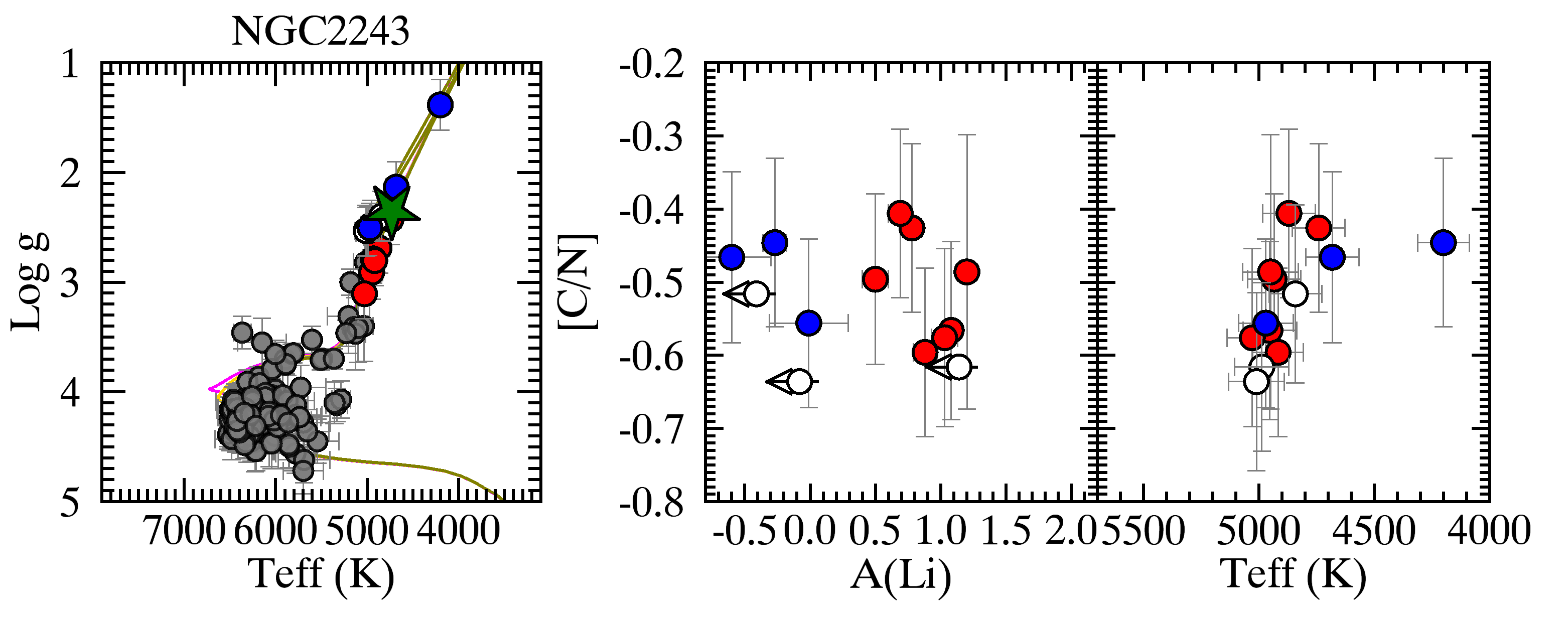
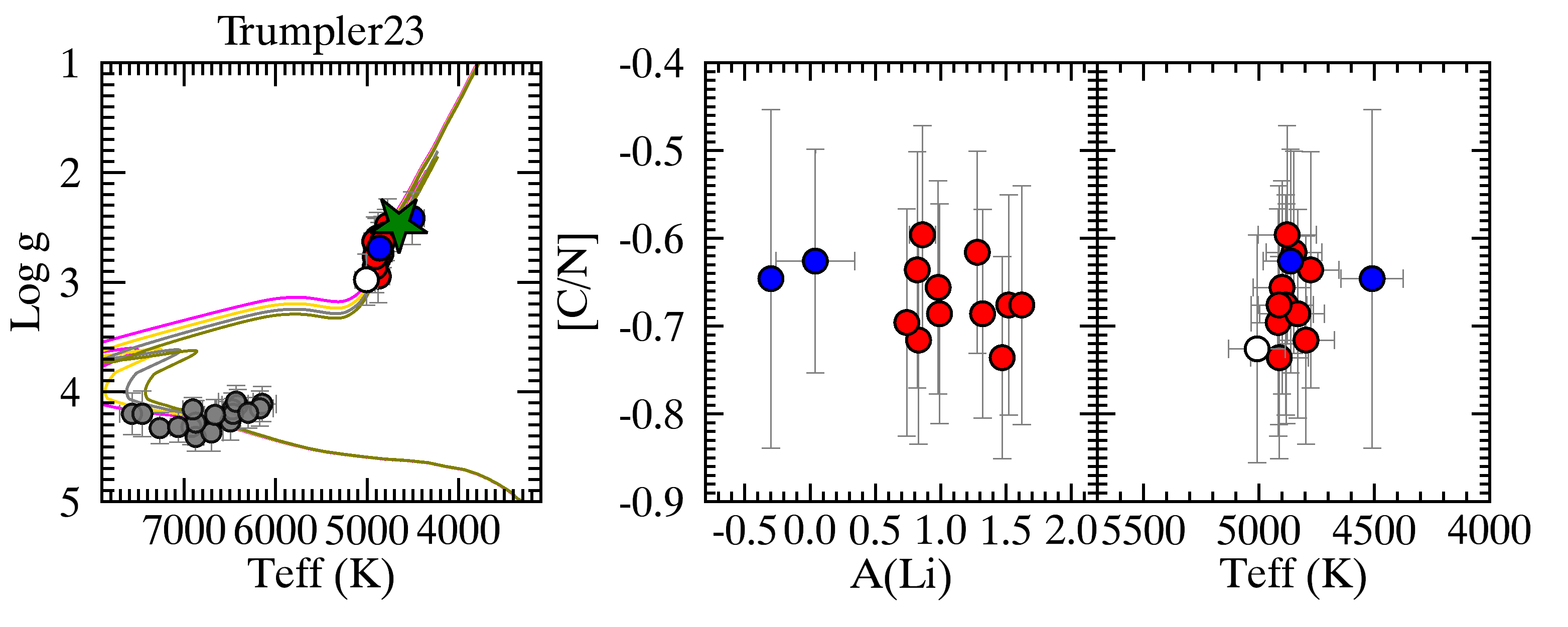
Figure 3: GES clusters NGC 2243 and Trumpler 23: log $g$-T_eff diagrams with PISA isochrones 3.7, 4.0, 4.3, 4.5 Gyr and 0.7, 0.8, 0.9, 1.0 Gyr, respectively (left panels), and member stars beyond the FDU, A(Li) vs [C/N] (central panel), and [C/N] abundance vs T_eff (right panel). Stars with A(Li)$>$0.4 are shown with red circles, stars with A(Li)$<$0.4 with blue circles, stars with upper limits measurements of A(Li) are indicated with empty circles and stars no-RGB or without C and N are shown with grey circles. The green star represents the position of the RGB bump.

In Figure 4 (in Figs. 19, 20, 21, 22, 23 in the Appendix we present all clusters) we show the log $g$-T_eff diagram (left panel) and [C/N] abundance vs T_eff (right panels) in giant stars of the APOGEE sample of open clusters for two example clusters. For these clusters, we do not have information on Li abundance. We thus use the information on the location on the log $g$-T_eff diagram and the variation of [C/N] to exclude stars for our final sample: basically we exclude stars beyond the RGB-bump but only if their [C/N] differs more than 1-$\sigma$ from the average [C/N] of the stars located before the bump.

From stellar evolution theory, we would expect that more evolved stars than the FDU to have lower [C/N] values if extramixing processes are in place (see, e.g. Lagarde et al. 2012). For some clusters we observe an opposite effect with at least one star more evolved along the isochrone having a higher [C/N] abundance (see, e.g., NGC6705, NGC6866) than the stars located at the clump. This unexpected result might be due to incorrect stellar parameters or abundances. These stars are not considered in the final average values. In addition, in many clusters (see, e.g. NGC 2420, Tr5, NGC 6819) we removed several stars (blue circles) which are probably non members, both for their location, quite far from the best fit isochrone, and for their discrepant [C/N]. They are not considered to compute the final average value.

Globally, the effect of the extramixing seems to be very limited in the metallicity range of open clusters: there is not a clear and systematic correlation between the location of a RGB star in the log $g$-T_eff diagram and the [C/N] value. There are some clusters for which this effect is appreciable, as for instance NGC 6791, in which many stars above the bump are observed and they have all systematically lower [C/N] abundances, while in other clusters, as, e.g., NGC 6819, the stars above the bump show similar [C/N] as the clump stars. In addition, where Li abundance is available, there is not a strong correlation of Li depletion with lower [C/N] values, as expected as a consequence of an extramixing episode. Only for the oldest clusters, we observe a [C/N] decrease for stars with A(Li)$<$0.4 dex, resulting from a more efficient dredge-up or thermohaline extra-mixing (see, e.g., Berkeley 31 and Berkeley 26). On the other hand, for younger clusters A(Li)$<$0.4 dex is often coupled with higher values of [C/N] with respect to stars with A(Li)$>$0.4 dex (see, for instance, NGC 6005, Rup 134, Pismis 18, Trumpler 23). This can be related to the higher mass of their evolved stars in which thermohaline instability does not occur (Lagarde et al. 2019). Thus, the mechanisms of Li-depletion can be uncorrelated to those that modify the C and N abundances. The latter can be related to rotation-induced mixing that has an impact on the internal chemical structure of main sequence stars, observable during the RGB phase (see. e.g. Charbonnel & Lagarde 2010). The anti-correlation in young clusters between A(Li) and [C/N] in Li-depleted stars cannot easily be explained by the current models and deserve further investigation and it is, perhaps, associated to the Li abundance owned in the main sequence and inherited during the following evolutionary phases.

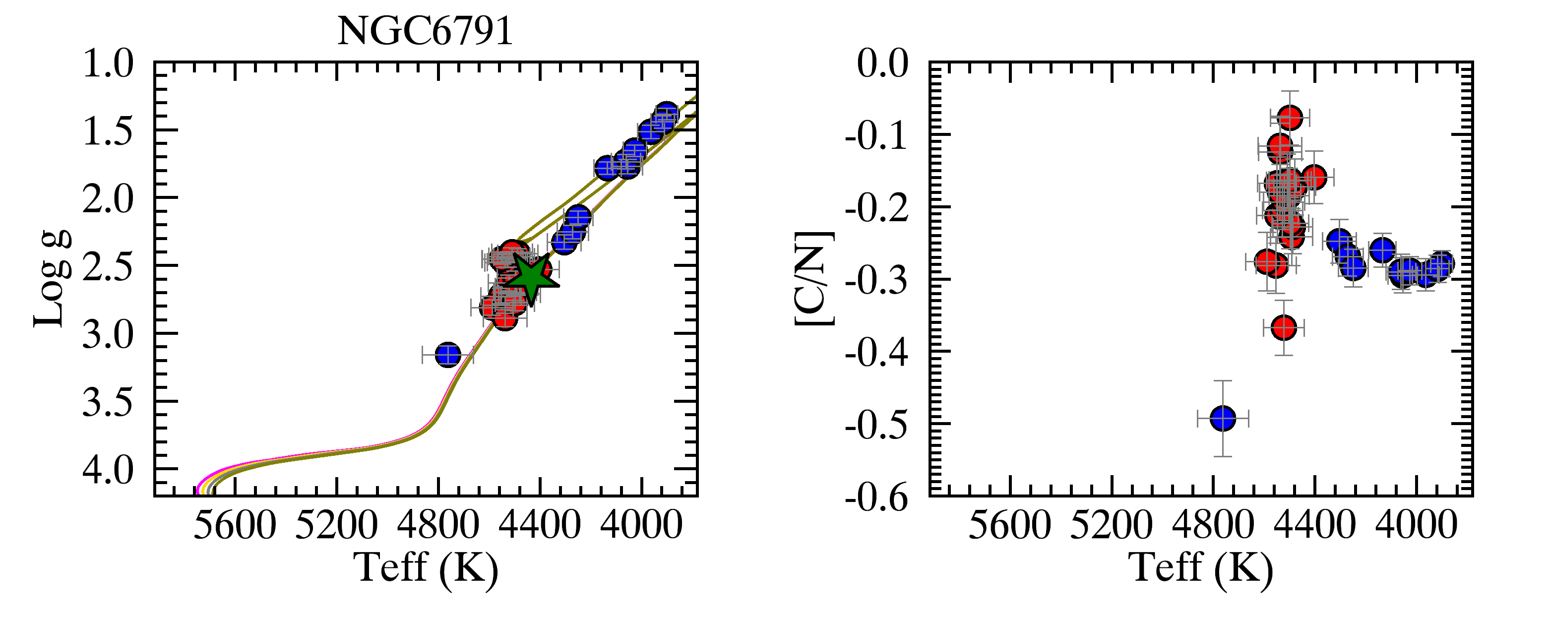
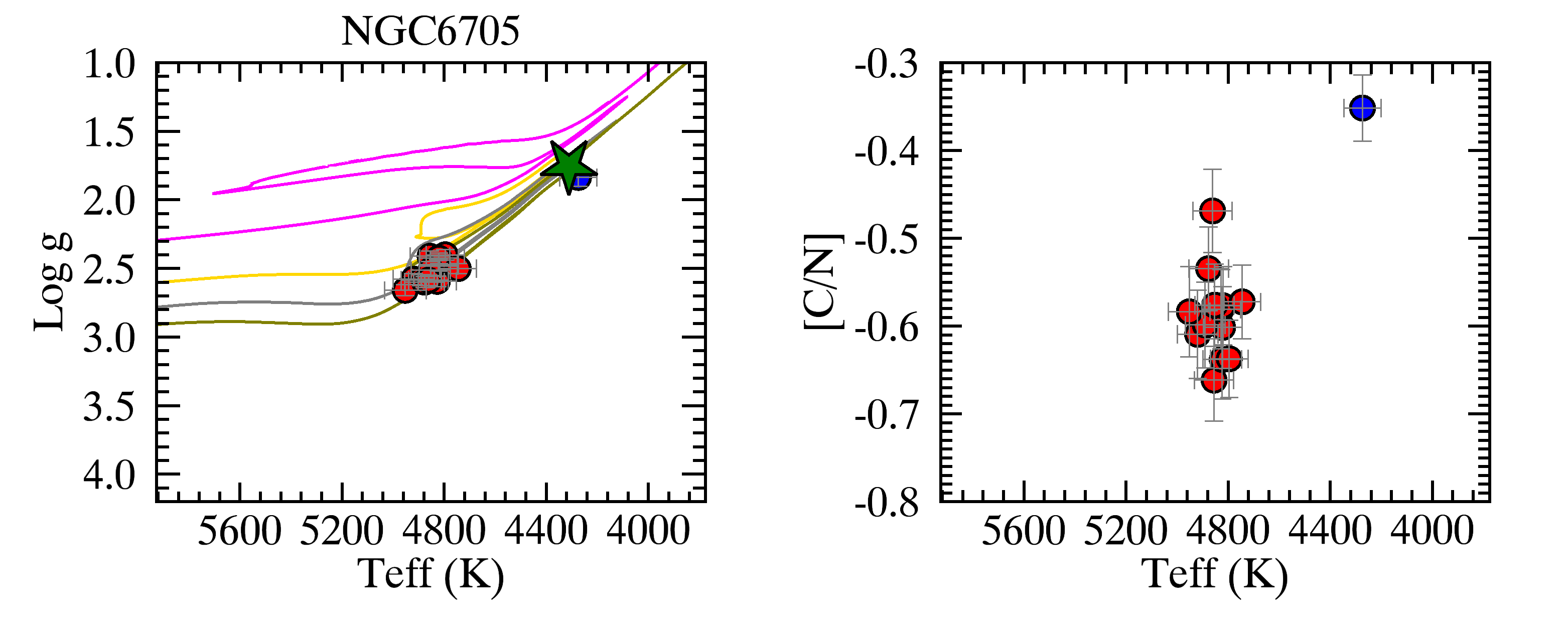
Figure 4: APOGEE clusters NGC 6791 and NGC 6705: log $g$-T_eff diagrams with PISA isochrones 7.3, 7.6, 7.9, 8.2 Gyr for NGC 67091 and 0.1, 0.2, 0.3, 0.4 Gyr for NGC 6705 (left panels) and [C/N] abundance vs T_eff (right panels). Symbols and colours as in Figure 3.

4 The Age-[C/N] relationship using open clusters

Table 4: Mean post-FDU [C/N] of the open clusters in the GES and APOGEE samples.

Open Clusters	[C/N]	# member stars	P${}_{memb.}^{mean}$
	(dex)
GES
Berkeley 31	$-0.32\pm 0.12$	1	0.87
Berkeley 36	$-0.30\pm 0.26$	1	0.89
Berkeley 44	$-0.38\pm 0.12$	2	1.00
Berkeley 81	$-0.64\pm 0.04$ (0.07)	11	0.99
Melotte71	$-0.65\pm 0.09$	2
NGC 2243	$-0.51\pm 0.05$ (0.08)	7	1.00
NGC 6005	$-0.64\pm 0.04$ (0.05)	9	0.97
NGC 4815a	$-0.70\pm 0.11$ (0.11)	5
NGC 6067	$-0.87\pm 0.04$ (0.08)	9	0.99
NGC 6259	$-0.84\pm 0.04$ (0.04)	12	0.99
NGC 6802	$-0.67\pm 0.04$ (0.08)	7	1.00
Rup134	$-0.63\pm 0.05$ (0.06)	16	0.98
Pismis18	$-0.74\pm 0.05$ (0.03)	5	0.99
Trumpler23	$-0.68\pm 0.04$ (0.04)	9	1.00
Trumpler20a	$-0.60\pm 0.12$ (0.12)	42
APOGEE
Berkeley 17	$-0.24\pm 0.02$ (0.06)	7
Berkeley 53	$-0.52\pm 0.03$ (0.05)	4
Berkeley 66	$-0.36\pm 0.03$ (0.08)	4
Berkeley 71	$-0.66\pm 0.04$ (0.18)	7
FSR0494	$-0.60\pm 0.04$ (0.09)	5
IC166	$-0.69\pm 0.02$ (0.20)	15
King 5	$-0.57\pm 0.03$ (0.01)	5
King 7	$-0.53\pm 0.03$ (0.04)	3
NGC 1193	$-0.44\pm 0.04$ (0.09)	3
NGC 1245	$-0.64\pm 0.02$ (0.11)	23
NGC 1798	$-0.44\pm 0.02$ (0.06)	8
NGC 188	$-0.32\pm 0.01$ (0.04)	10
NGC 2158	$-0.41\pm 0.02$ (0.13)	18
NGC 2420	$-0.40\pm 0.02$ (0.07)	11
NGC 6791	$-0.20\pm 0.01$ (0.06)	19
NGC 6811	$-0.68\pm 0.03$ (0.01)	4
NGC 6819	$-0.49\pm 0.01$ (0.03)	14
NGC 6866	$-0.69\pm 0.03$ (0.06)	6
Teutsch 51	$-0.58\pm 0.06$ (0.04)	4
Trumpler 5	$-0.37\pm 0.02$ (0.04)	9
NGC 7789	$-0.52\pm 0.01$ (0.03)	17
GES and APOGEE
M67-GES	$-$0.37$\pm$0.07 (0.06)	3
M67-APOGEE dr14	$-$0.57$\pm$0.01 (0.07)	23
M67-APOGEE dr14b	$-$0.50$\pm$0.09	21
M67-adopted (dr14b-GES)	$-$0.43$\pm$0.11	$-$
NGC 6705-GESa	$-$0.69$\pm$0.09	27
NGC 6705-APOGEE dr14	$-$0.60$\pm$0.01 (0.03)	12
NGC 6705-adopted	$-$0.64$\pm$0.09	$-$

In Table 6, we present the results of our analysis: the mean [C/N] abundance ratio of the member giant stars (with selection criteria described in the previous sections) and the number of used stars for each cluster in both the GES and APOGEE samples. The uncertainties in Table 6 are the formal errors on the weighted mean and, within brackets, the standard deviation $\sigma$, and they take into account of uncertainties on C and N abundances. Using the solar values from Grevesse et al. (2007), we compute the average [C/N] ratio in each cluster in the GES sample, while for APOGEE clusters the solar-scaled abundance ratios are already given in their database. For three clusters of the GES sample, Trumpler 20, NGC 6705 and NGC 4815, we use their literature [C/N] estimated only for post-FDU stars from Tautvaišienė et al. (2015) based on GES results (C and N abundances are not re-derived in next data releases, therefore they are not present in GES idr4 and idr5, used in the present work).

There are two clusters in common between the two surveys, M67 and NGC 6705, that can be used to cross-calibrate the [C/N] abundances in the two surveys, together with few other stars in common, mainly benchmark stars.

In M67, there are three stars in common between GES and APOGEE with [C/N] abundances. The average post-FDU abundance in M67, using APOGEE dr14, is [C/N]=$-$0.57$\pm$0.01, while the GES results give [C/N]=$-$0.37$\pm$0.07. The C and N abundances of stars in M67 along the evolutionary sequence have been studied in details by Bertelli Motta et al. (2017) using APOGEE dr12. Their post-FDU stars have an average [C/N]= $-$0.46$\pm$0.03, which is in good agreement with the expectation of theoretical models for stars of mass and metallicity of the evolved stars of M67 (Salaris et al. 2015), as shown in their Figure 9. The results for M67 in APOGEE dr14 are slightly higher, due to an offset in the [C/N] abundances from APOGEE dr12 to the latest APOGEE dr14 release. In Fig. 5 we compare [C/N] in three stars in common between APOGEE (dr12, dr14) and GES. The [C/N] values of APOGEE dr14 are systematically lower than those in dr12. The values of GES and APOGEE dr12 are in better agreement (close to the 1-to-1 relationship). We notice that a recent paper (Souto et al. 2019) re-analyzed 83 APOGEE dr14 spectra of stars in M67. The analysis performed in this paper is more accurate than the standard one (K. Cunha, S. Hasselquist, private communication). There are five stars in common between GES and the sample of Souto et al. (2019), two of them with C and N abundances. For these stars the agreement in [C/N] is within 0.01 dex. We thus use the re-analysis of Souto et al. (2019) to compute the mean [C/N] of giant stars after the FDU in M67, which is [C/N]=$-$0.50$\pm$0.09. In the following analysis, we adopt for M67 an average between the GES and the results of Souto et al. (2019).

The other cluster in common between the two surveys is NGC 6705. In Fig. 6 we show the [C/N] abundances in stars in common between APOGEE (dr12 and dr14) and GES. As for M67, the [C/N] values of APOGEE d14 are systematically lower than those in dr12. On the other hand, for this cluster the values of dr14 are in much better agreement with the GES results.

In the following analysis, we adopt for NGC 6705 an average between the GES from Tautvaišienė et al. (2015) and the APOGEE dr14 results.

To identify possible systematic offsets or trends, we make a global cross-match between APOGEE dr12 and dr14 and GES. In Fig. 7 we show the [C/N] abundances of stars in common between GES and the two APOGEE releases. We notice a general better agreement of APOGEE dr14 with GES, while the [C/N] abundances in APOGEE dr12 are usually offset of $\sim$0.2 dex.

In the plot of Fig. 7, we highlight the abundances of the three stars of M67. These stars are indeed outliers in the APOGEE dr14, with a negative offset with respect to GES. For the stars we use the improved analysis of Souto et al. (2019) as suggested by the APOGEE team (K. Cunha, S. Hasselquist, private communication).

For the other stars, there are no systematic offsets and the agreement between the two sets of results is, within the errors, good. This allows us to securely combine the GES and APOGEE dr14 samples of clusters (with the exception of the results of M67, for which we adopt the Souto et al. (2019)’s results).

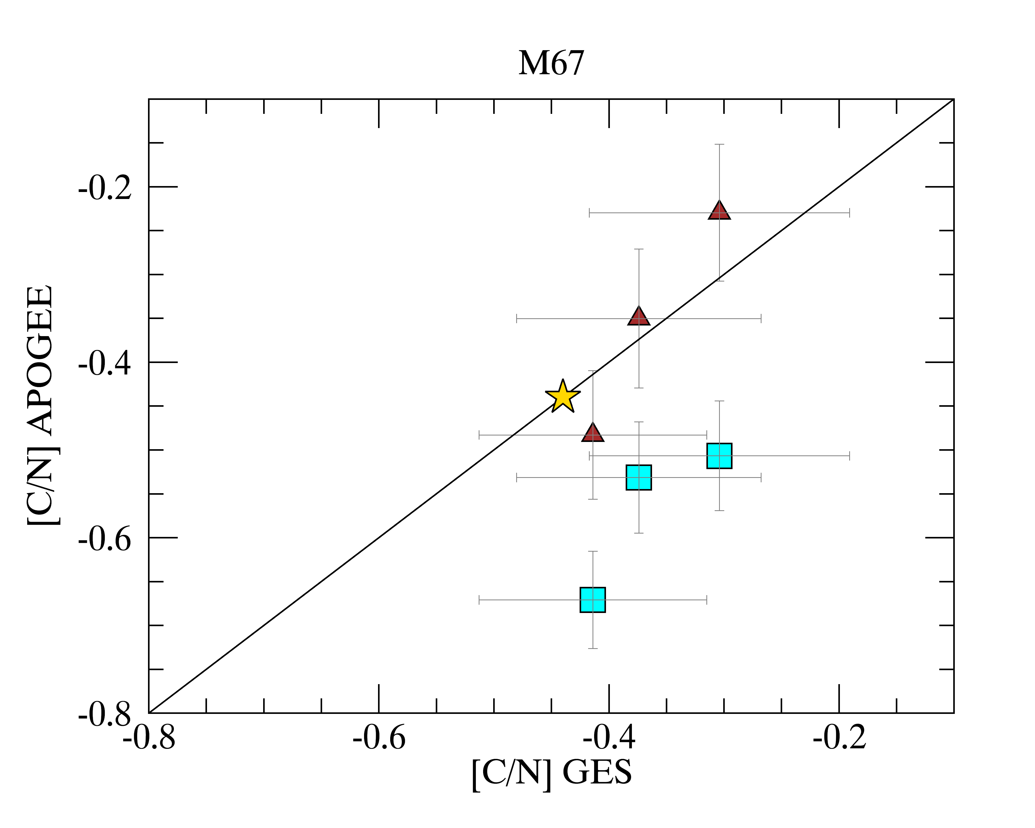
Figure 5: Stars in common between GES and APOGEE (dr12– brown triangles and dr14 –cyan squares) in M67. The continuous line is the 1-to-1 relation. The yellow stars is the theoretical location of the FDU in the models of Salaris et al. (2015) for the age and metallicity of M67.

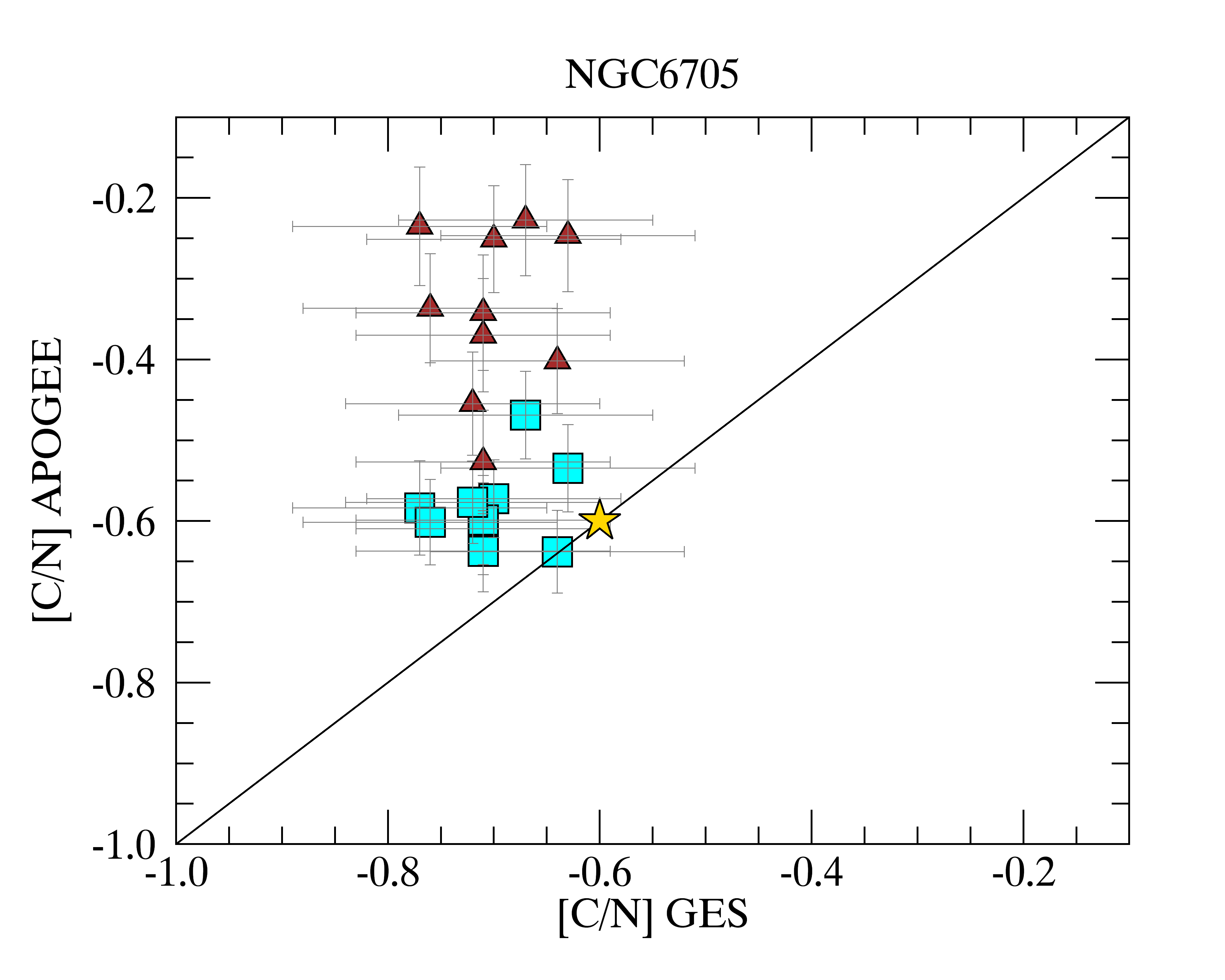
Figure 6: Stars in common between GES and APOGEE (dr12– brown triangles and dr14 –cyan squares) in NGC 6705. The continuous line is the 1-to-1 relation. The yellow stars is the theoretical location of the FDU in the models of Salaris et al. (2015) for the age and metallicity of NGC 6705.

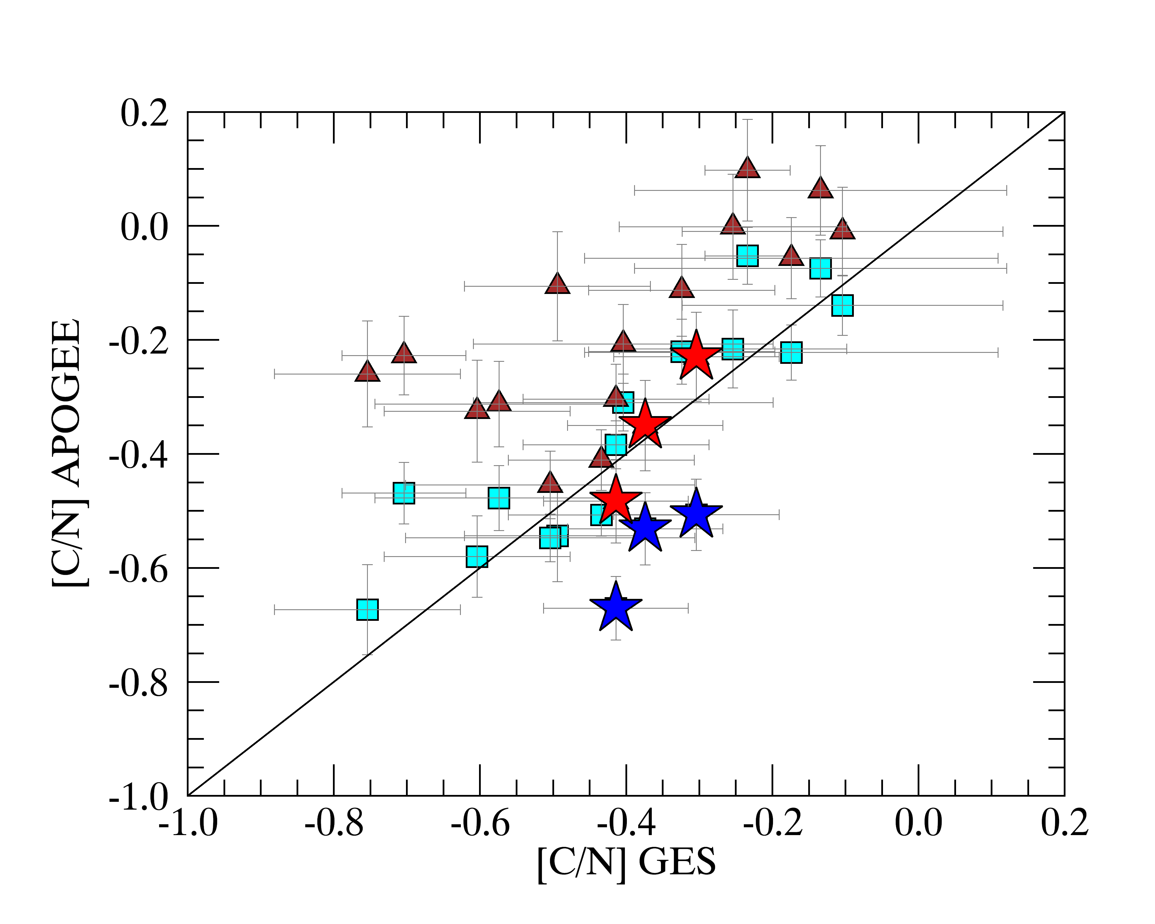
Figure 7: Stars in common between GES and APOGEE (dr12– brown triangles and dr14 –cyan squares). The continuous line is the 1-to-1 relation. The red stars are the abundances in M67 for APOGEE dr12 and the blue stars for APOGEE dr14.

In Figure 8, we show the relationship between [C/N] in GES and APOGEE clusters and their logarithmic ages.

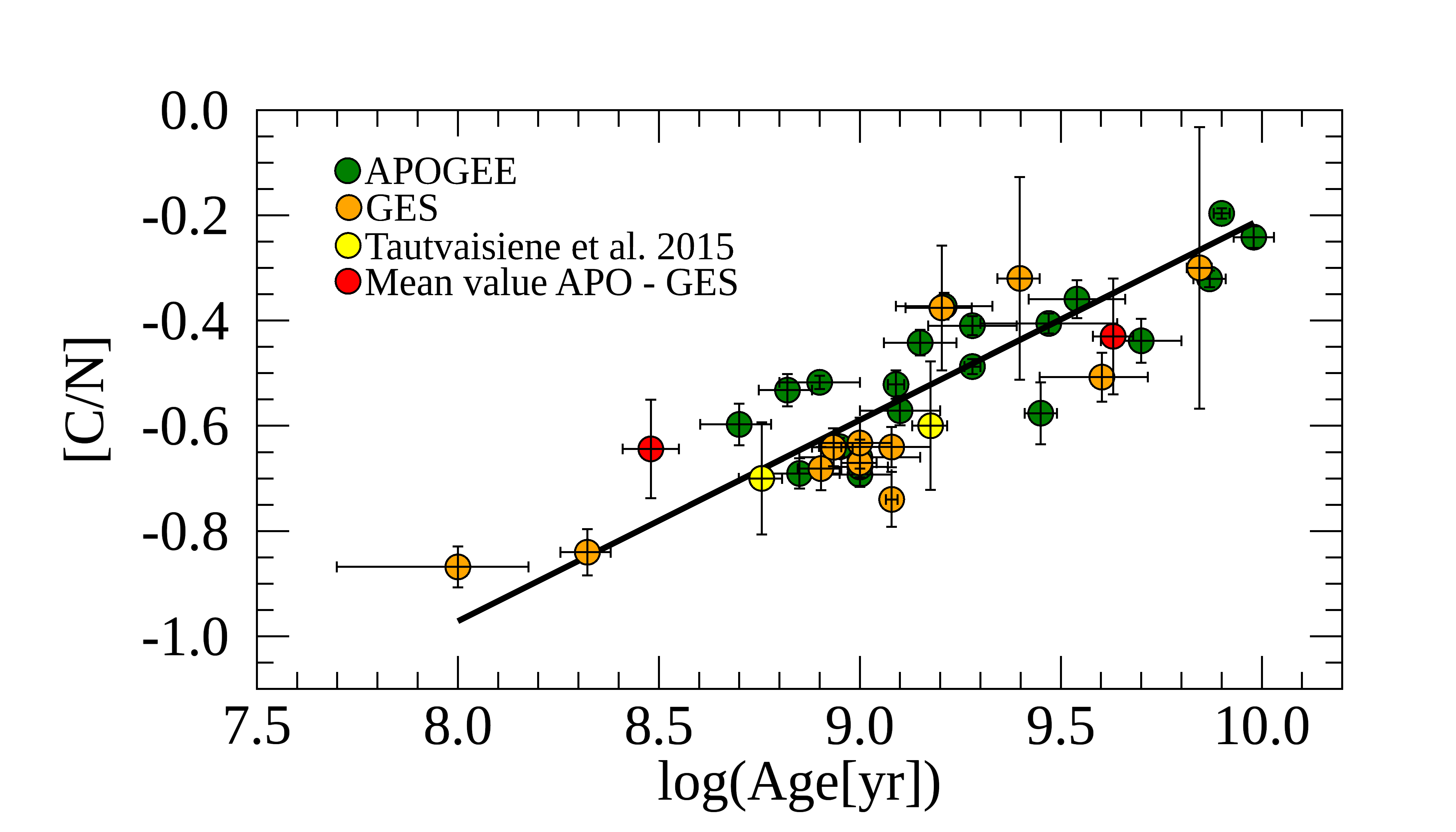
Figure 8: Average [C/N] ratios of cluster member stars with $\log$ g cut as a function of $\log$(Age[yr]) for the GES (orange circles) and the APOGEE (green circles) surveys. The yellow circles are the GES literature results by Tautvaišienė et al. (2015). The red circles represent the mean value [C/N] for NGC 6705 and M67. The straight line is the linear weighted least-squares fit of data.

With the ages expressed in logarithmic form the relationship is linear, with a Pearson coefficient R=0.85, and it has the following expression

$$\log[\rm Age(yr)]=10.54(\pm 0.06)+2.61(\pm 0.10){\rm[C/N]}$$ (1)

This relationship has important implication, because, if we know the evolutionary stage of a giant star and we can measure its [C/N] abundance ratio, we can infer its age. However, there are some caveats that need to be explicitly discussed here: i) the relationship in Eq.1 is empirical and it is built using open clusters whose metallicity range is $-$0.4$<$[Fe/H]$<$+0.4. Thus, its application outside this [Fe/H] range is not correct. ii) At low metallicity, the effect of non-canonical extra-mixing in post-FDU stars increases and thus the measured [C/N] loses its dependence on stellar mass (and thus age). iii) Although the ages of giant stars are poorly constrained by isochrone fitting, and thus their age estimate through Eq. 1 is a step forwards, the uncertainties on [C/N]-ages are still high, as we discuss in the next paragraphs.

4.1 Error estimate

It is known that the measurements of stellar ages are usually affected by large uncertainties. However, accurate knowledge of stellar ages is a fundamental constraint for the scenarios of the formation and evolution of the different components of our Galaxy. Astroseismology data from CoRoT and Kepler have improved our knowledge of stellar ages, but they are limited to still small samples of stars. In this framework, chemical clocks, as [C/N] but also [Y/Mg] and [Y/Al] (Tucci Maia et al. 2016; Spina et al. 2016; Feltzing et al. 2017; Spina et al. 2018; Delgado Mena et al. 2018), might be important auxiliary tools because they can be obtained for large numbers of stars. However, it is important to have a clear idea of the uncertainties related to the use of abundance ratios to derive the age of a star.

From the GES results, the typical uncertainties on the C and N abundances are 0.05 dex and 0.065 dex, respectively, with a typical uncertainties on the abundance ratio [C/N] of $\sim$0.10 dex. They affect the uncertainties on $\rm\log(Age[yr])$ giving a mean value of about $\sim$0.26 dex on the logarithm of the age. These uncertainties translate into $\sim$55-60% for the linear ages. For the APOGEE results, the typical uncertainties on the C and N abundances are $\sim$0.04 dex and $\sim$0.04 dex, respectively, with a typical uncertainty on the abundance ratio [C/N] of $\sim$0.06 dex. As for GES, this implies a mean uncertainty on logarithm of the age of $\sim$0.17 dex and of $\sim$40-45% for the linear ages. Typical uncertainties are shown in Table 5.

Table 5: Typical uncertainties on logarithmic and linear age in different range of logarithmic age.

log(Age[yr])	e(log(Age[yr]))	e(Age)%
GES
8.0-8.5	0.24	55%
8.5-9.0	0.26	60%
9.0-9.5	0.26	60%
9.5-10.0	0.26	60%
APOGEE
8.0-8.5	0.19	45%
8.5-9.0	0.19	45%
9.0-9.5	0.17	40%
9.5-10.0	0.17	40%

However, another important part in the error budget is the uncertainty in the parameters of the fit of the linear relationship of Eq. 1. Combining both GES and APOGEE sample, we lower the uncertainties on the slope and on the intercept of the linear relationship. At the moment, the uncertainties on the parameters of the fit are of the order of $\sim$0.06 and $\sim$0.10 on the intercept and slope, respectively. We expect to have a more accurate fit of the relationship at GES completion, when about 70 open clusters will be available. At the moment, the age estimate with [C/N] abundance can be considered as an additional tool to give an independent estimate of the age of field stars, in particular for giant stars whose age determination through isochrone fitting is not appropriate due to the little separation of isochrones of different ages.

4.2 Comparison with previous results

A relationship between logarithmic age and [C/N] was already provided for the APOGEE catalogue: Martig et al. (2016) presented an empirical relationship between [C/N] and stellar masses (and thus stellar ages) based on the asteroseismic mass estimates from the APOKASC survey (a spectroscopic follow-up by APOGEE of stars with asteroseismology data from the Kepler Asteroseismic Science Consortium, Borucki et al. 2010). To compare with our results, we cross-matched the APOKASC catalogue of Martig et al. (2016) with APOGEE dr14, and we find the mean offset between the dr12 and dr14 abundances. We apply the offset to the dr12 APOKASC abundances to have them on the same scale as our clusters.

In Fig. 9 we plot the ages from Martig et al. (2016) and [C/N] measurements from dr12 (scaled to dr14), together with the results of our sample of the open clusters and the relation of Eq.1. We note that the two samples have different slopes at older ages, where the effect of extra-mixing might be higher. In the oldest regime ($\log$[Age]$>$9.5), the ages obtained by Martig et al. (2016) are $\sim$ 0.2 dex younger than ours at fixed [C/N]. Mackereth et al. (2017) showed that Martig et al. (2016) underestimated the ages in the older regime by up to a factor of 2 when compared with those based on asteroseismological masses. Therefore, our relationship provide ages in better agreement with those of Mackereth et al. (2017).

For the youngest ages, at a given [C/N] our ages correspond to [C/N] values close to the APOGEE dr12 re-scaled ones, although with a large dispersion. This is true in the region where the two samples overlap, even if the APOKASC sample does not populate the youngest-ages regions, where many star clusters are located, reaching a lower limit of about $\log$[Age]$\sim$8.8.

The combination of ages from asteroseismology with those from isochrone fitting in young open clusters deserve to be investigated and to be fully exploited to obtain a calibration of the [C/N]-Age relation in a wider age range.

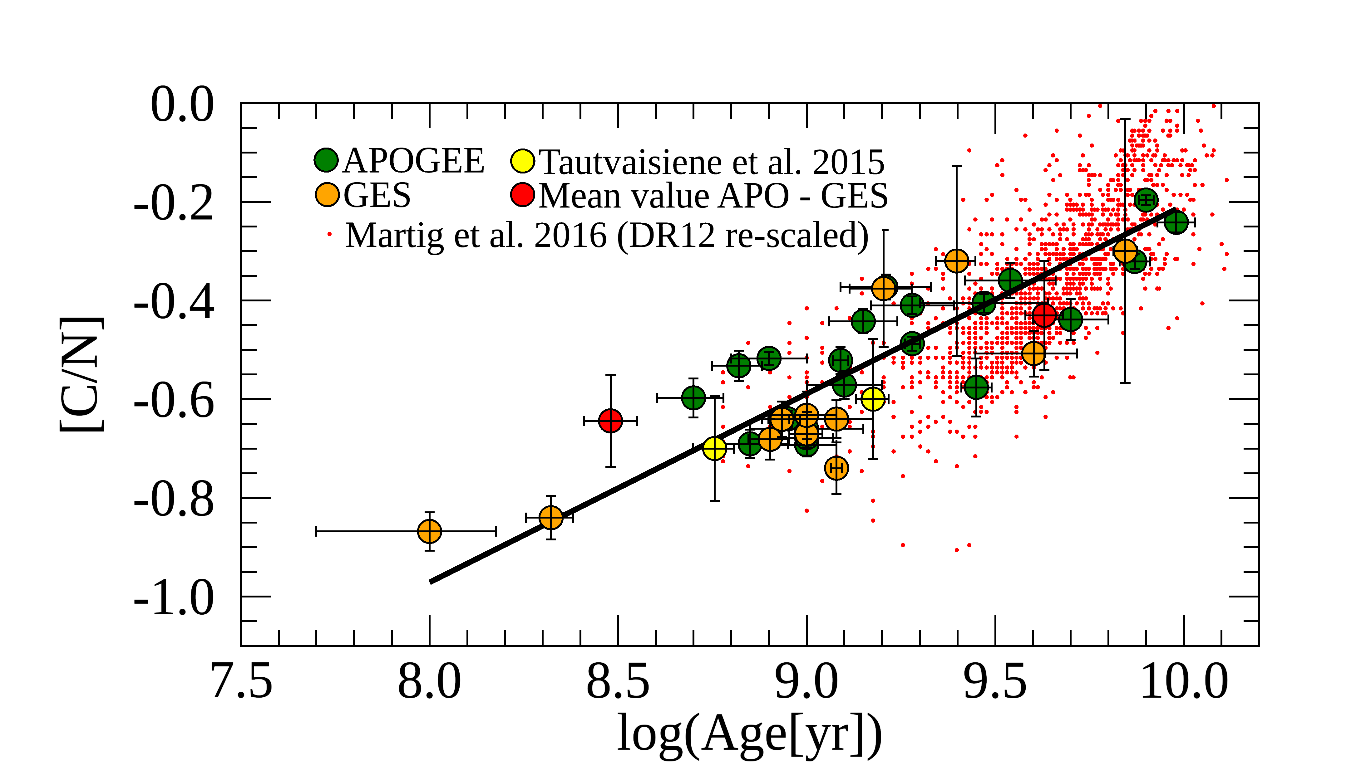
Figure 9: Comparison between the field stars in APOKASC with [C/N] vs age computed by Martig et al. (2016) (dr12 small red dots and dr14 small blue dots) and those obtained in the present work using open clusters in the APOGEE and GES surveys (symbols and colour-codes as in Fig. 8).

5 Comparison with theoretical models

Later phases of stellar evolution affect the abundances of C and N, and therefore the abundances of these elements do not trace the initial chemical composition of stars, but they are modified by stellar nucleosynthesis and by internal mixing. In this framework, it is of interest to compare with predictions of various theoretical models of stellar evolution, having in mind the limits of such comparison, such as: i) not perfect correspondence between the stellar models used for the isochrones adopted to derive the ages of open clusters and those adopted to predict surface [C/N] abundances; ii) possible offsets in [C/N] between models and observations ; iii) comparison of different kinds of stars in model and observations.

We compare our results with models in two different ways: a classical comparison with a set of standard stellar evolution models, computed for different metallicities (Salaris et al. 2015) and a more innovative approach that combines a stellar population synthesis model of the Galaxy with a complete grid of stellar evolution models (Lagarde et al. 2017).

In Fig. 10, we compare the observed [C/N] ratio at the FDU vs. age with theoretical predictions of Salaris et al. (2015). We recall that in our observations we select giant stars beyond the FDU, avoiding stars after the RGB bump with measurable effects of extra-mixing in their [C/N] abundances and/or Li-depleted. The models of Salaris et al. (2015) are computed with the BaSTI stellar library (Pietrinferni et al. 2004, 2006) and they include the effect of the overshooting. The theoretical curves give the [C/N] abundance after the FDU at a given stellar age. They are provided for different metallicities in the age range 1-10 Gyr. We select three curves covering the metallicity range of our sample clusters.

The data of open clusters follow the general trend of the models, confirming the predicted increase in [C/N] with age. In the age range where both observations and models are available we have colour-coded them in the same way to facilitate the association of the observations with the corresponding curves. There is a general agreement with model curve and observations within the uncertainties, but no trend with metallicity can be seen for the observations.

In Fig. 11 we compare our data with the results of the model of Lagarde et al. (2017) for three ranges of metallicities. The models of Lagarde et al. (2012) have been applied to an improved stellar population model of the Galaxy by Lagarde et al. (2017), providing global, chemical and seismic properties of the thin-disc stellar population. They estimate the effect of the thermohaline mixing in thin-disc giants, which produce measurable effects on the [C/N] ratios of stars of different metallicities. They derive mean relations between [C/N] and age, usable to estimate ages for thin-disc red-clump giants as a function of their [Fe/H]. Since the open clusters are a thin-disc population and we mainly select low-RGB and RC stars in them, we can compare our results with the models of Lagarde et al. (2017).

The data are in qualitative agreement with the model curves of Lagarde et al. (2017), which, however, predict lower [C/N] values for the oldest stars. On the other hand, the open cluster data are in better agreement with the model curves of Salaris et al. (2015), whose models show an increasing [C/N] abundance with age which better follows the observed trend in the oldest clusters. Both models are computed for ages$>$1 Gyr, and for different metallicities (in the plot we show the models computed for the metallicity range of our sample of clusters). In the data, at a given age, we do not distinguish between trends of clusters with different metallicities. However, in the metallicity range spanned by the data, model predictions would differ only of $\sim$0.1 dex considering the two metallicity extremes. This difference is comparable with typical [C/N] uncertainty.

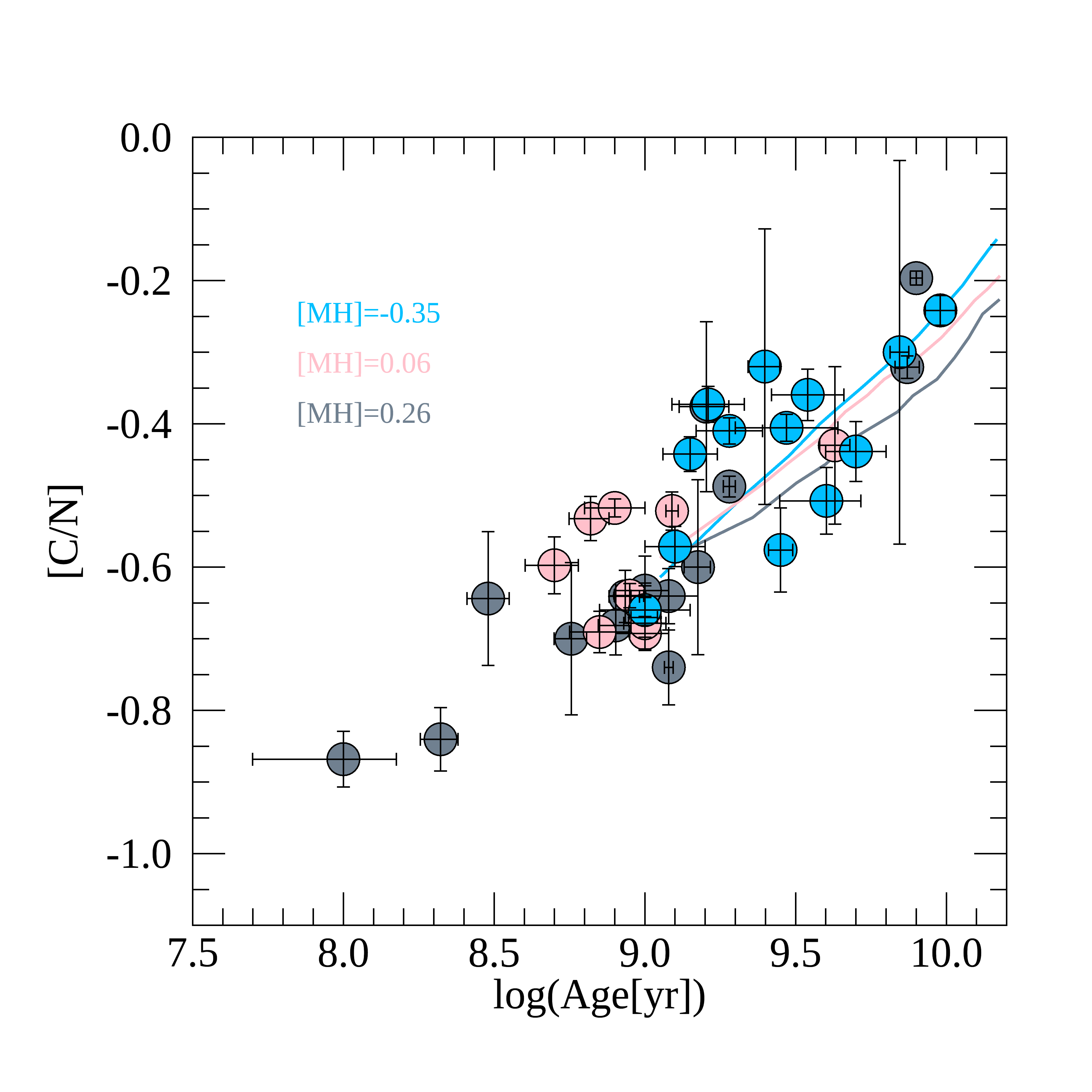
Figure 10: Comparison of [C/N] and age between the theoretical models by (Salaris et al. 2015) and the open clusters in GES and APOGEE surveys. The models are computed for different metallicities. Their colour-codes are shown in the legend. The clusters are divided in three metallicity bins: [Fe/H]$\leq-0.10$ (light blue circles), $-0.1\leq$ [Fe/H] $\leq+0.1$ (pink circles), and [Fe/H] $\geq+0.1$ (grey circles).

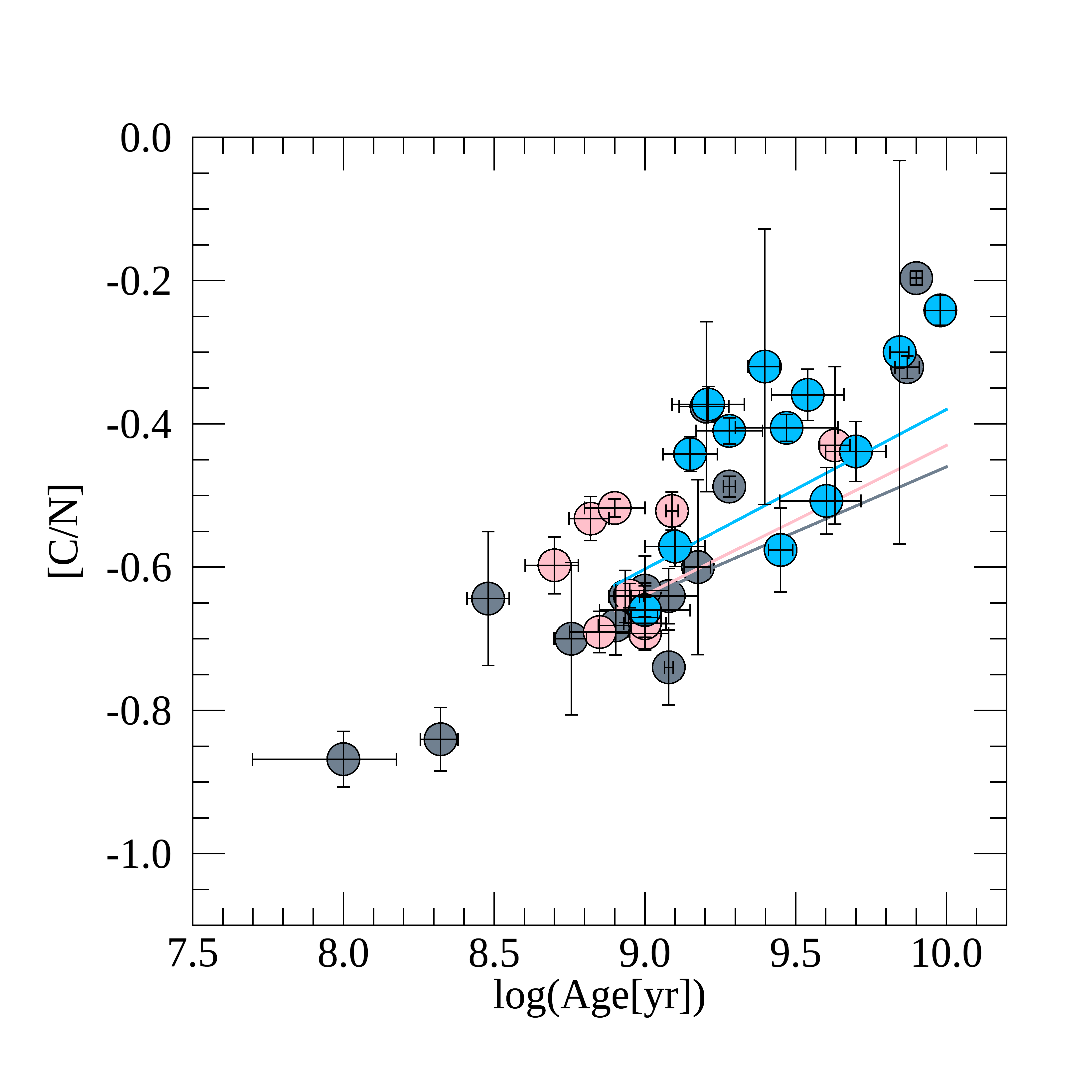
Figure 11: Comparison between age and [C/N] of the thin-disc RC giant modelled by Lagarde et al. (2017) (continuous lines - light blue, pink and grey) and the clusters in GES and APOGEE. The clusters and models are divided in three metallicity bins: [Fe/H]$\leq-0.10$ (light blue circles), $-0.1\leq$ [Fe/H] $\leq+0.1$ (pink circles), and [Fe/H] $\geq+0.1$ (grey circles).

6 Application to field stars

As mentioned by Masseron & Gilmore (2015), passing from [C/N] measurements to assign masses and ages is tempting, but at the same time it is risky because of several unknown or underestimated effects, such as, for instance, the exact evolutionary stage of each observed stars, the metallicity dependence of C and N abundances after the FDU, and the effect of the extra-mixing at different ages and metallicities (cf. Lagarde et al. 2017).

Keeping in mind these limits, we combine the sample of giant stars in the GES and APOGEE databases with C and N abundances aiming at identifying age trends along the disc populations. Among giant stars, we select stars which have passed the FDU. To identify the maximum log $g$ at which the FDU can appear, we consider our grid of isochrones (Pisa isochrones, Dell’Omodarme et al. 2012) at different ages and metallicities. For each of them we derive the value of log $g$ corresponding to the point where [C/N] starts to monotonically decrease, i.e., log $g$ (FDU). For most of the field stars, which are usually older than the cluster stars, the mean value of surface gravity at the FDU is log $g$ $\sim$3.4, with a little dependence on metallicity (see Fig. 1). We also excluded stars above the RGB-bump (considering the most conservative case of stars of 2-3 Gyr, the age of the bulk of the stars in our sample, for which the RGB-bump is located at log $g$ $\sim$2.4). Therefore, in the following analysis, we select giant field stars with 2.4$<$ log $g$ $<$3.4. In addition, we use the line-of-sight distances derived by Bailer-Jones et al. (2018b) with Gaia dr2. They use a distance prior that varies smoothly as a function of Galactic longitude and latitude according to a Galaxy model. We apply the relationship of Eq. 1 to giant field stars taking into account its limits of applicability: $-$0.4$<$[Fe/H]$<$+0.4 and 0.1 Gyr$<$age$<$10 Gyr, range of metallicity and age of clusters studied in this work.
There are about 52 000 giant stars – of which $\sim$ 264 belonging to GES – in the our combined sample for which we can estimate the age. Thanks to the distance obtained with Gaia, we can locate them in the Galaxy. With our determination of stellar ages, we can investigate the age trends in the thin- and thick-disc populations.

In Fig. 12, we show [$\alpha$/Fe] vs. [Fe/H] for the APOGEE and GES sample, colour-coded by their [C/N] abundance ratio. The dichotomy between the $\alpha$-enhanced thick stars and the lower [$\alpha$/Fe] thin disc is evident also in terms of their [C/N]. As already observed by Masseron & Gilmore (2015) in their analysis of the APOGEE catalogue for dr12, we can see a clear gradient in [C/N], with the thin disc stars having a lower [C/N]. At a given metallicity, [C/N] becomes larger for higher [$\alpha$/Fe] (see also Hasselquist et al. 2019). The gradient in [C/N] can then be translated into a gradient in ages, as shown in Fig. 13. In this plot there are two approximations: i) the relationship of Eq. 1 has been applied outside the range of metallicity -0.4$<$[Fe/H]$<$+0.4 and also to thick disc stars, with different [$\alpha$/Fe] and thus different initial [C/Fe]; ii) stars with derived age $>$10 Gyr are shown in red. Their ages are estimated applying the relationship outside its range of applicability and, for this reason, they do not represent a correct age estimate and we can just say they are old. There is a clear division in age between thin and thick disc stars: we can see that the youngest stars are present in the thin disc and their ages become greater with the increase of the $\alpha$-elements content. The thick disc stars are in general older than the thin disc ones. Most of them have only lower limits estimate of their ages, with age $\gtrsim$ 10 Gyr.

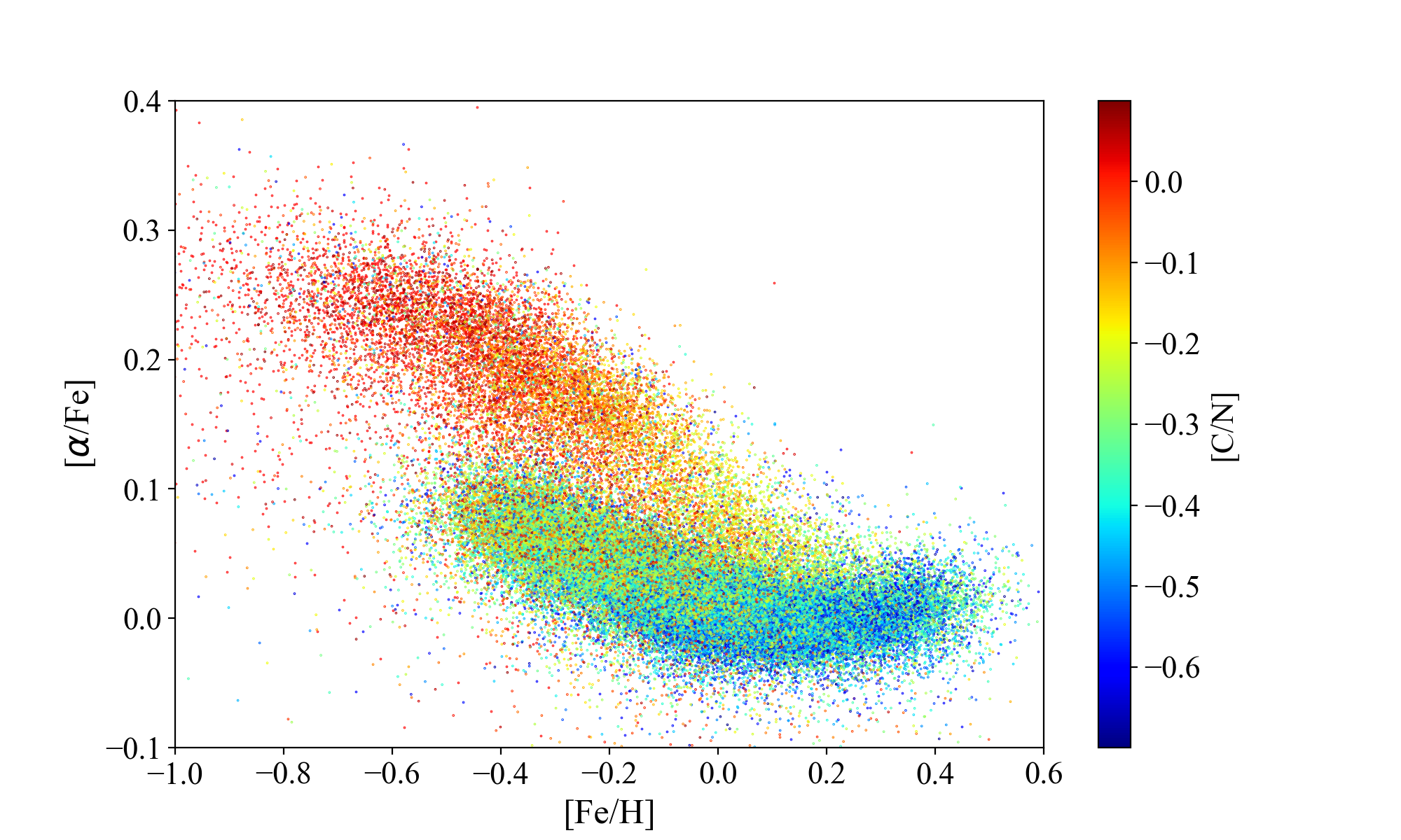
Figure 12: [$\alpha$/Fe] as a function of [Fe/H] for field stars in the APOGEE dr14 and a GES samples. The stars are colour-coded by [C/N].

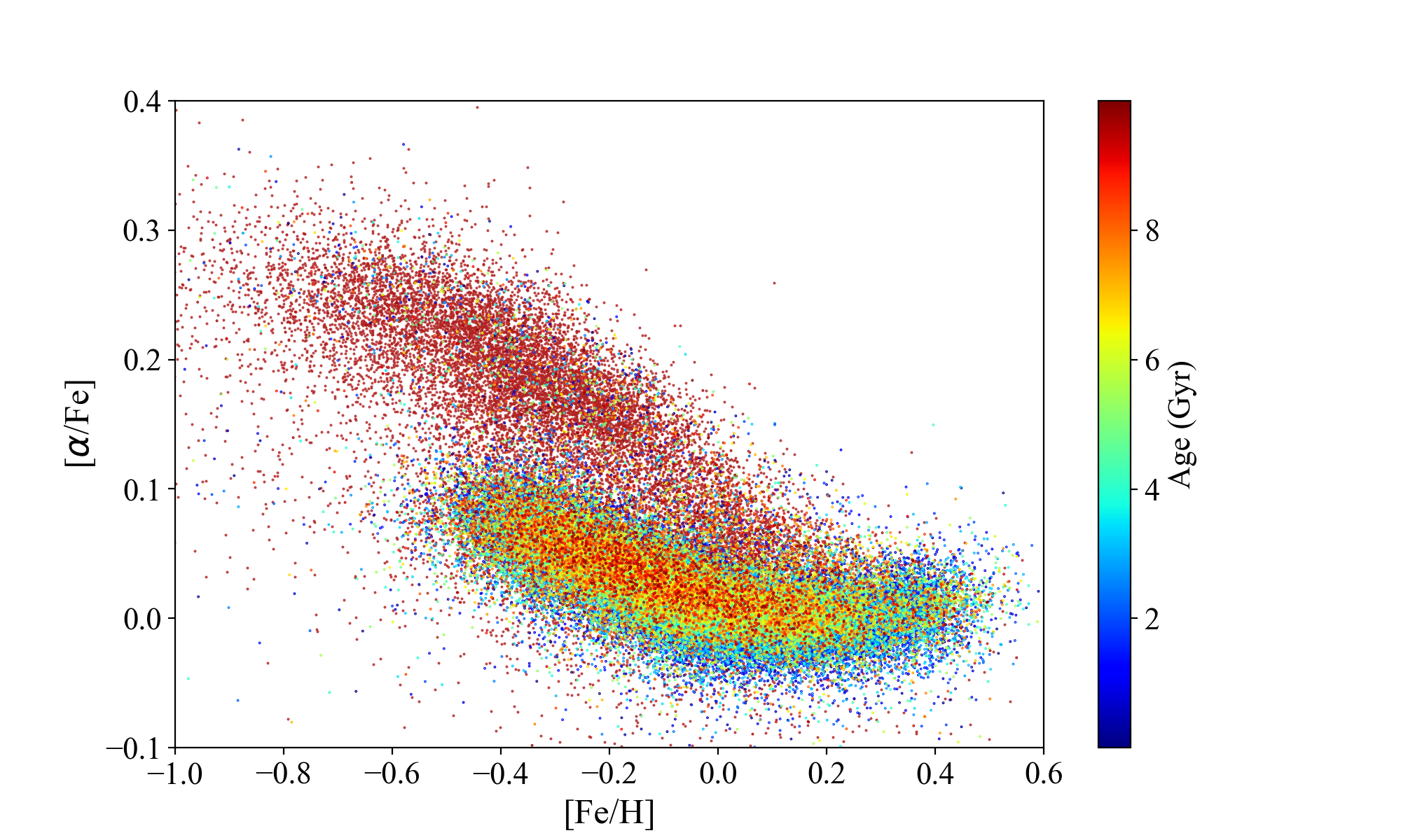
Figure 13: [$\alpha$/Fe] as a function of [Fe/H] for field stars in the APOGEE dr14 and a GES samples. The stars are colour-coded by ages.

In Fig 14, we present the histogram of the derived stellar ages in different bins of $\rm\left|z\right|$ and R_GC, covering a radial region 3 ¡ R_GC ¡ 15 kpc, and a vertical region $\rm\left|z\right|$ ¡ 2 kpc. We divide our sample in several radial and vertical regions, as done by Hayden et al. (2015). In this plot, and in the following Table 6 and Fig. 15, we apply the relationship of Eq. 1 in the metallicity range $-$0.4$<$[Fe/H]$<$+0.4 and we do not include lower limit measurements. In Table 6, we show the median ages and $\sigma$ in each bin. The bins close to the Plane contain the youngest stars, but they have also a non negligible tail of old stars. The stars located in the bins at intermediate height are older, and, even more, stars located at 1 kpc$<|z|<$2 kpc. This is appreciable also from Table 6 where a systematic increasing age is observed for stars located above the Galactic Plane. In the bins characterizing the thin disc 0 kpc$<|z|<$0.5 kpc, the youngest population is located in the inner bins, and the ages slightly increase towards the outskirts.

In Fig. 15, we show the [$\alpha$/Fe] vs. [Fe/H] plane dividing in same bins as in Fig. 14. For smaller z, the thin-disc population, characterized by a low-[$\alpha$/Fe], is prominent. Instead, for larger z, the population of thick disc starts to increase, being more prominent in the inner regions.

The bottom panels of Fig. 15 show the thin-disc population closer to the plane. In the 3 kpc ¡R_GC¡ 7 kpc ranges the populations is dominated by thin disc metal-rich stars, where the stars with the highest metallicity are youngest ones. As we can see from the histograms of the age distribution in each bin in $\rm\left|z\right|$ and R_GC in Fig. 14 and respective medians and $\sigma$ in Table 6, the population in 3 kpc ¡R_GC¡ 7 kpc at low z is mainly young. Therefore, the inner bin is dominated by young and metal rich stars, with low [$\alpha$/Fe]. Moving towards the outer regions 7 kpc ¡R_GC¡ 11 kpc, the thin disc includes a wider range of [Fe/H], from $-$0.4 to 0.4. Following our age estimate, the younger stars are located in the lower envelope of the distribution, at low [$\alpha$/Fe]. There is a consistent number of old stars with both super- and sub-solar metallicity. In the outer regions, 11 kpc ¡R_GC¡ 15 kpc the metal-rich stars start to disappear.

The central panels of Fig. 15 show the thin-disc population at intermediate height above the plane. In the innermost regions 3 kpc¡R_GC¡7 kpc the thin disc is poorly populated, unlike the region 7 kpc¡R_GC¡11 kpc. This effect is due to the observational selection of APOGEE survey, for which the observations are located in particular towards the outer regions at 7-11 kpc if compared with the inner ones at 3-7 kpc. The stars in these two panels do not reach the low [$\alpha$/Fe] and the young ages of the corresponding panels at lower z. Indeed, their median ages are older than the medians at the same R_GC, but lower z (see Table 6). In the outer regions, there are fewer metal-rich stars, and on average they are younger, as their medians show if compared with ones in the inner regions at intermediate z (see Table 6).

The top panels of Fig. 15 show the thin disc population at high height above the plane. Stars are almost absent from the innermost regions, due to the sample selection in the range of applicability of our relationship, from which, they would be older than 10 Gyr. From 7 to 11 kpc, there is signature of thin disc stars with a wide age range. Finally, in the outermost regions 11-15 kpc few young and intermediate-age thin disc stars are present.

Table 6: Median and $\sigma$ of the age for each bin in height on the plane z and Galactocentric distance R_GC.

RGC (kpc)	$\rm\left|z\right|$ (kpc)	Median age (Gyr)	$\sigma$
3 $-$ 5	1 $-$ 2	2.95	2.95
5 $-$ 7	1 $-$ 2	5.06	2.81
7 $-$ 9	1 $-$ 2	5.80	2.69
9 $-$ 11	1 $-$ 2	5.34	2.61
11 $-$ 13	1 $-$ 2	4.00	2.57
13 $-$ 15	1 $-$ 2	4.06	2.34
3 $-$ 5	0.5 $-$ 1	4.20	2.87
5 $-$ 7	0.5 $-$ 1	4.79	2.57
7 $-$ 9	0.5 $-$ 1	4.23	2.50
9 $-$ 11	0.5 $-$ 1	3.98	2.39
11 $-$ 13	0.5 $-$ 1	3.75	2.42
13 $-$ 15	0.5 $-$ 1	3.97	2.44
3 $-$ 5	0 $-$ 0.5	1.82	2.53
5 $-$ 7	0 $-$ 0.5	2.32	2.44
7 $-$ 9	0 $-$ 0.5	2.63	2.35
9 $-$ 11	0 $-$ 0.5	3.05	2.28
11 $-$ 13	0 $-$ 0.5	3.17	2.40
13 $-$ 15	0 $-$ 0.5	3.04	2.45

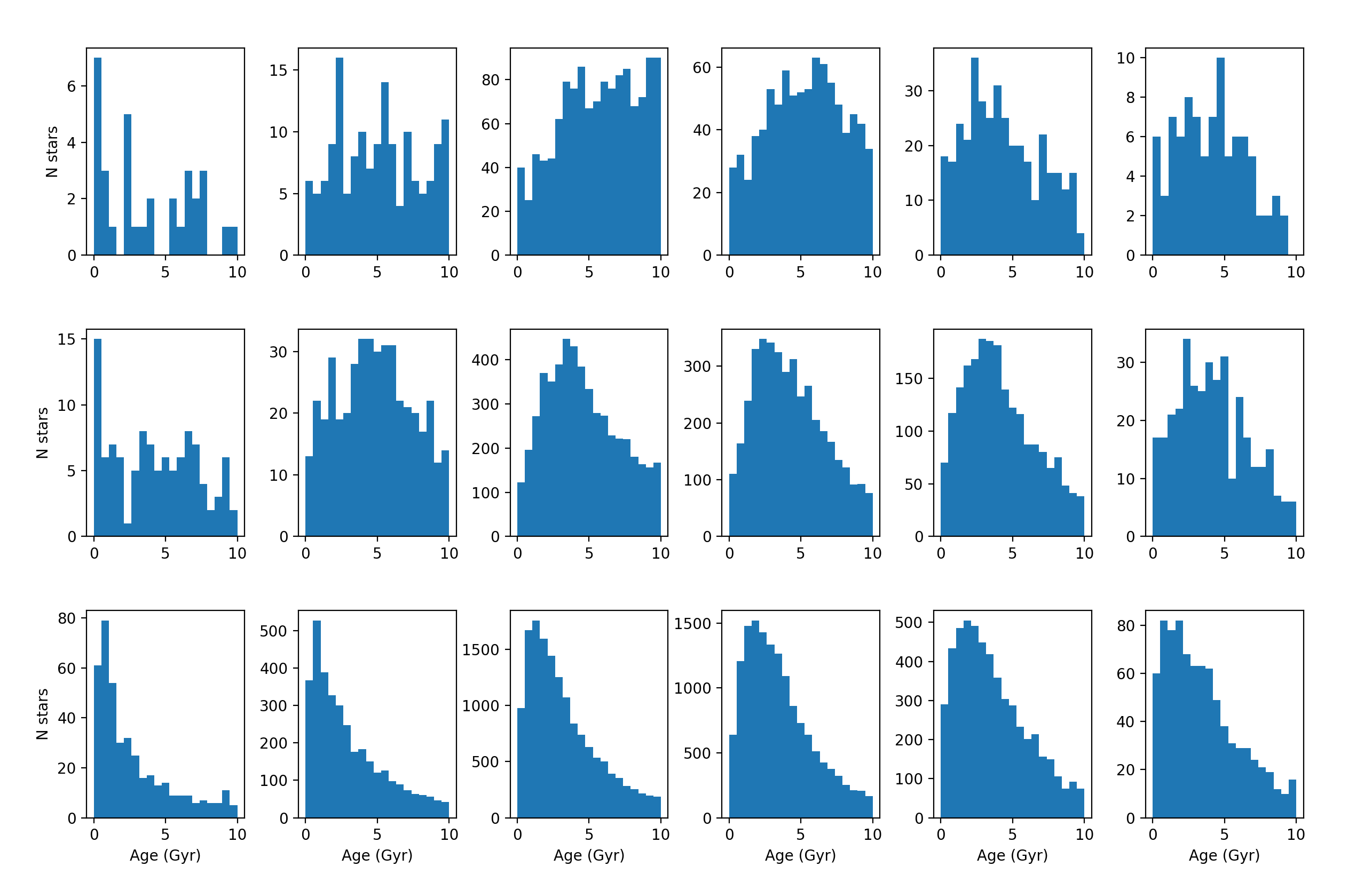
Figure 14: Histograms of the age for each bin in height on the plane $\rm\left|z\right|$ and Galactocentric distance R_GC. Each panel is corrispondent to the respective one in Fig. 15.

7 Summary and conclusions

The databases of stellar spectra from high-resolution spectroscopic surveys, as GES and APOGEE, are providing extremely wide and accurate data-sets of stellar parameters and abundances for large samples of stars in the different Galactic components. Some abundance ratios, such as, for instance, [C/N], [Y/Mg], [Y/Al], [Ba/Fe] have been recognised to be powerful chemical clocks, i.e., strictly related to the stellar ages. In particular, the [C/N] abundance ratio is a good age indicator for stars in the RGB evolutionary phase after the first dredge-up. Using open clusters in the GES and APOGEE Surveys, we calibrate a relationship between cluster age (from isochrone fitting of the whole cluster sequence) and [C/N] abundance ratio of stars that have passed the FDU. We carefully select RGB stars beyond the FDU, studying the effects of extra-mixing process in their [C/N] abundances. We compare the [C/N] measurements and ages of open clusters with the predictions of stellar evolutionary models by Salaris et al. (2015) and Lagarde et al. (2017), finding a good agreement, but with the current accuracy of age and abundance measurements we cannot confirm the variation of the age-[C/N] relationship with metallicity in the [Fe/H] range traced by open clusters.

We use our relationship to derive the ages of field stars in a combined GES and APOGEE sample. In the plane [$\alpha$/Fe] vs. [Fe/H], we see a clear dichotomy between the [C/N] abundances in the thin and thick disc as already observed by Masseron & Gilmore (2015), and consequently stellar ages. We extrapolate our relation to estimate the ages for thin disc stars and giving lower limit ages for the thick disc stars. As expected, we find that stars belonging to the thin disc are on average younger than the stars in the thick disc. Typical age of the thin disc stars decreases going into the inner part of the disc at low z and towards the outskirts. The former indicates that the metal rich stars in the inner disc represent the later phases of the Galactic evolution, while the latter is expected from an inside-out formation of the disc.

These immediate applications of the relationships between ages and [C/N] probe the power of chemical clocks to improve our knowledge of stellar ages. The next step will be to estimate in a homogeneous way the age of the open clusters in the final data release of GES survey to put them on a common stellar age scale. In addition, we plan to combine other chemical clocks, as for instance [Ba/Fe] or [Y/Mg] to give further constraints to the ages of stars in different evolutionary stages.

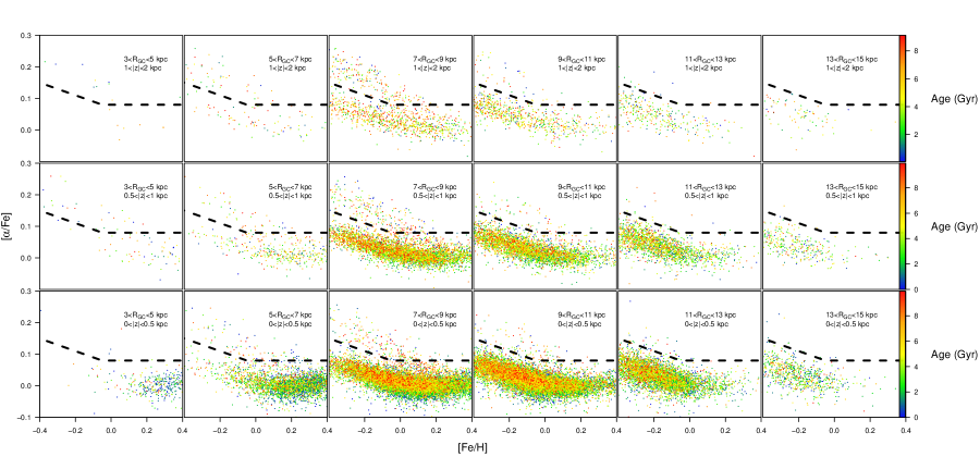
Figure 15: [$\alpha$/Fe] as a function of [Fe/H] for field stars in the APOGEE sample. The stars are colour coded by ages. The dashed line shows the separation between thin and thick disc populations. Each plot contains stars selected by means of Galactocentric radius R_GC and height z, labeled in each figure.

Appendix A Appendix

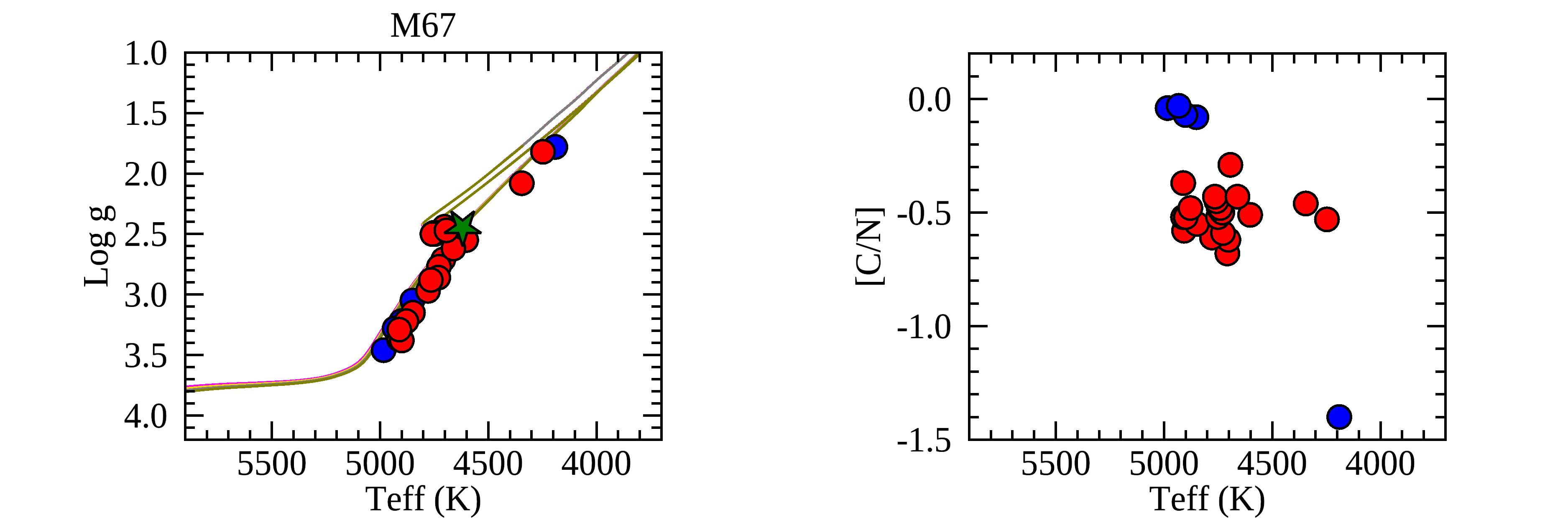
Figure 24: log $g$-T_eff diagram with PISA isochrones (left panel) and [C/N] abundance vs T_eff (right panel) of M67 by (Souto et al. 2019). Symbols and colours as in Figure 4. The used isochrones are 3.8, 4.0, 4.2, 4.4 Gyr.