STRASS: A Light and Effective Method for Extractive Summarization
Based on Sentence Embeddings

Abstract

This paper introduces STRASS: Summarization by TRAnsformation Selection and Scoring. It is an extractive text summarization method which leverages the semantic information in existing sentence embedding spaces. Our method creates an extractive summary by selecting the sentences with the closest embeddings to the document embedding. The model learns a transformation of the document embedding to minimize the similarity between the extractive summary and the ground truth summary. As the transformation is only composed of a dense layer, the training can be done on CPU, therefore, inexpensive. Moreover, inference time is short and linear according to the number of sentences. As a second contribution, we introduce the French CASS dataset, composed of judgments from the French Court of cassation and their corresponding summaries. On this dataset, our results show that our method performs similarly to the state of the art extractive methods with effective training and inferring time.

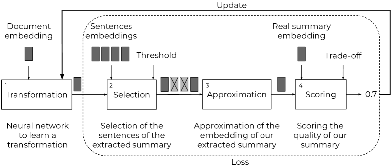
Figure 1: Training of the model. The blocks present steps of the analysis. All the elements above the blocks are inputs (document embedding, sentences embeddings, threshold, real summary embedding, trade-off).

1 Introduction

Summarization remains a field of interest as numerous industries are faced with a growing amount of textual data that they need to process. Creating summary by hand is a costly and time-demanding task, thus automatic methods to generate them are necessary. There are two ways of summarizing a document: abstractive and extractive summarization.

In abstractive summarization, the goal is to create new textual elements to summarize the text. Summarization can be modeled as a sequence-to-sequence problem. For instance, Rush et al. (2015) tried to generate a headline from an article. However, when the system generates longer summaries, redundancy can be a problem. See et al. (2017) introduce a pointer-generator model (PGN) that generates summaries by copying words from the text or generating new words. Moreover, they added a coverage loss as they noticed that other models made repetitions on long summaries. Even if it provides state of the art results, the PGN is slow to learn and generate. Paulus et al. (2017) added a layer of reinforcement learning on an encoder-decoder architecture but their results can present fluency issues.

In extractive summarization, the goal is to extract part of the text to create a summary. There are two standard ways to do that: a sequence labeling task, where the goal is to select the sentences labeled as being part of the summary, and a ranking task, where the most salient sentences are ranked first. It is hard to find datasets for these tasks as most summaries written by humans are abstractive.Nallapati et al. (2016a) introduce a way to train an extractive summarization model without labels by applying a Recurrent Neural Network (RNN) and using a greedy matching approach based on ROUGE. Recently, Narayan et al. (2018b) combined reinforcement learning (to extract sentences) and an encoder-decoder architecture (to select the sentences).

Some models combine extractive and abstractive summarization, using an extractor to select sentences and then an abstractor to rewrite them Chen and Bansal (2018); Cao et al. (2018); Hsu et al. (2018). They are generally faster than models using only abstractors as they filter the input while maintaining or even improving the quality of the summaries.

This paper presents two main contributions. First, we propose an inexpensive, scalable, CPU-trainable and efficient method of extractive text summarization based on the use of sentence embeddings. Our idea is that similar embeddings are semantically similar, and so by looking at the proximity of the embeddings it is possible to rank the sentences. Secondly, we introduce the French CASS dataset (section 4.1), composed of 129,445 judgments with their corresponding summaries.

2 Related Work

In our model, STRASS, it is possible to use an embedding function trained with state of the art methods.

Word2vec is a classical method used to transform a word into a vector Mikolov et al. (2013a). Methods like word2vec keep information about semantics Mikolov et al. (2013b). Sent2vec Pagliardini et al. (2017) create embedding of sentences. It has state-of-the-art results on datasets for unsupervised sentence similarity evaluation.

EmbedRank Bennani-Smires et al. (2018) applies sent2vec to extract keyphrases from a document in an unsupervised fashion. It hypothesizes that keyphrases that have an embedding close to the embedding of the entire document should represent this document well.

We adapt this idea to select sentences for summaries (section 4.2). We suppose that sentences close to the document share some meaning with the document and are sentences that summarize well the text. We go further by proposing a supervised method where we learn a transformation of the document embedding to an embedding of the same dimension, but closer to sentences that summarize the text.

3 Model

The aim is to construct an extractive summary. Our approach, STRASS, uses embeddings to select a subset of sentences from a document.

We apply sent2vec to the document, to the sentences of the document, and to the summary. We suppose that, if we have a document with an embedding $\mathbf{d}$ and a set $S$ with all the embeddings of the sentences of the document, and a reference summary with an embedding $\mathbf{ref\_sum}$, there is a subset of sentences $E_{S}\subset S$ forming the reference summary. Our target is to find an affine function $f(\cdot)$: ${\rm I\!R^{\mathit{n}}}\longrightarrow{\rm I\!R^{\mathit{n}}}$, such that:

$$\begin{cases}sim(\mathbf{s},f(\mathbf{d}))\geq t&\text{if }\mathbf{s}\in E_{S}\\ sim(\mathbf{s},f(\mathbf{d}))<t,&\text{otherwise}\end{cases}$$

Where $t$ is a threshold, and $sim$ is a similarity function between two embeddings.

The training of the model is based on four main steps (shown in Figure 1):

• (1) Transform the document embedding by applying an affine function learned by a neural network (section 3.1);

• (2) Extract a subset of sentences to form a summary (section 3.2);

• (3) Approximate the embedding of the extractive summary formed by the selected sentences (section 3.3);

• (4) Score the embedding of the resulting summary approximation with respect to the embedding of the real summary (section 3.4).

To generate the summary, only the first two steps are used. The selected sentences are the output. Approximation and scoring are only necessary during the training phase when computing loss function.

3.1 Transformation

To learn an affine function in the embedding space, the model uses a simple neural network. A single fully-connected feed-forward layer. $f(\cdot)$: ${\rm I\!R^{\mathit{n}}}\longrightarrow{\rm I\!R^{\mathit{n}}}$:

$$\begin{multlined}f(\mathbf{d})=\mathbf{W}\times\mathbf{d}+\mathbf{b}\end{multlined}f(\mathbf{d})=\mathbf{W}\times\mathbf{d}+\mathbf{b}$$

with $\mathbf{W}$ the weight matrix of the hidden layer and $\mathbf{b}$ the bias vector. Optimization is only conducted on these two elements.

3.2 Sentence Extraction

Inspired by EmbedRank Bennani-Smires et al. (2018) our proposed approach is based on embeddings similarities. Instead of selecting the top $n$ elements, our approach uses a threshold. All the sentences with a score above this threshold are selected. As in Pagliardini et al. (2017), our similarity score is the cosine similarity. Selection of sentences is the first element:

$$\begin{multlined}sel(\mathbf{s},\mathbf{d},S,t)=\\ sigmoid(ncos^{+}(\mathbf{s},f(\mathbf{d}),S)-t)\end{multlined}sel(\mathbf{s},\mathbf{d},S,t)=\\ sigmoid(ncos^{+}(\mathbf{s},f(\mathbf{d}),S)-t)$$

with $sigmoid$ the sigmoid function and $ncos^{+}$ a normalized cosine similarity explained in section 3.5. A sigmoid function is used instead of a hard threshold as all the functions need to be differentiable to make the back-propagation. $Sel$ outputs a number between 0 and 1. 1 indicates that a sentence should be selected and 0 that it should not. With this function, we select a subset of sentences from the text that forms our generated summary.

3.3 Approximation

As we want to compare the embedding of our generated extractive summary and the embedding of the reference summary, the model approximates the embedding of the proposed summary. As the system uses sent2vec, the approximation is the average of the sentences weighted by the number of words in each sentence. We have to apply this approximation to the sentences extracted with $sel$, which compose our generated summary. The approximation is:

$$app(\mathbf{d},S,t)=\sum_{\mathbf{s}\in S}\mathbf{s}\times nb\_w(\mathbf{s})\times sel(\mathbf{s},\mathbf{d},S,t)$$

where, $nb\_w(\mathbf{s})$ is the number of words in the sentence corresponding to the embedding $\mathbf{s}$.

3.4 Scoring

The quality of our generated summary is scored by comparing its embedding with the reference summary embedding. Here, the compression ratio is added to the score in order to force the model to output shorter summaries. The compression ratio is the number of words in the summary divided by the number of words in the document.

$$\begin{multlined}loss=\lambda\times\frac{nb\_w(\mathbf{gen\_sum})}{nb\_w(\mathbf{d})}+\\ (1-\lambda)\times cos\_sim(\mathbf{gen\_sum},\mathbf{ref\_sum})\end{multlined}loss=\lambda\times\frac{nb\_w(\mathbf{gen\_sum})}{nb\_w(\mathbf{d})}+\\ (1-\lambda)\times cos\_sim(\mathbf{gen\_sum},\mathbf{ref\_sum})$$

with $\lambda$ a trade-off between the similarity and the compression ratio, $cos\_sim(\mathbf{x},\mathbf{y})$, $\mathbf{x},\mathbf{y}\in{\rm I\!R}^{n}$ the cosine similarity and $\mathbf{gen\_sum}=app(\mathbf{d},S,t)$. The user should note that $\lambda$ is also useful to change the trade-off between the proximity of the summaries and the length of the generated one. A higher $\lambda$ results in a shorter summary.

3.5 Normalization

To use a single selection threshold on all our documents, a normalization is applied on the similarities to have the same distribution for the similarities on all the documents. First, we transform the cosine similarity from $({\rm I\!R}^{n},{\rm I\!R}^{n})\longrightarrow[-1,1]$ to $({\rm I\!R}^{n},{\rm I\!R}^{n})\longrightarrow[0,1]$:

$$cos^{+}(\mathbf{x},\mathbf{y})=\frac{cos\_sim(\mathbf{x},\mathbf{y})+1}{2}$$

Then as in Mori and Sasaki (2002) the function is reduced and centered in $0.5$:

$$\begin{multlined}rcos^{+}(\mathbf{x},\mathbf{y},X)=\\ 0.5+\frac{cos^{+}(\mathbf{x},\mathbf{y})-\underset{\mathbf{x_{k}}\in X}{\operatorname{\mu}}(cos^{+}(\mathbf{x_{k}},\mathbf{y}))}{\underset{\mathbf{x_{k}}\in X}{\operatorname{\sigma}}(cos^{+}(\mathbf{x_{k}},\mathbf{y}))}\\ \end{multlined}rcos^{+}(\mathbf{x},\mathbf{y},X)=\\ 0.5+\frac{cos^{+}(\mathbf{x},\mathbf{y})-\underset{\mathbf{x_{k}}\in X}{\operatorname{\mu}}(cos^{+}(\mathbf{x_{k}},\mathbf{y}))}{\underset{\mathbf{x_{k}}\in X}{\operatorname{\sigma}}(cos^{+}(\mathbf{x_{k}},\mathbf{y}))}\\$$

where $\mathbf{y}$ is an embedding, $X$ is a set of embeddings, $\mathbf{x}\in X$, $\operatorname{\mu}$ and $\operatorname{\sigma}$ are the mean and standard deviation.

A threshold is applied to select the closest sentences on this normalized cosine similarity. In order to always select at least one sentence, we restricted our similarity measure in $(-\infty,1]$, where, for each document, the closest sentence has a similarity of 1:

$$\begin{multlined}ncos^{+}(\mathbf{x},\mathbf{y},X)=\frac{rcos^{+}(\mathbf{x},\mathbf{y},X)}{\underset{\mathbf{x_{k}}\in X}{\max}(rcos^{+}(\mathbf{x_{k}},\mathbf{y},X))}\end{multlined}ncos^{+}(\mathbf{x},\mathbf{y},X)=\frac{rcos^{+}(\mathbf{x},\mathbf{y},X)}{\underset{\mathbf{x_{k}}\in X}{\max}(rcos^{+}(\mathbf{x_{k}},\mathbf{y},X))}$$

4 Experiments

4.1 Datasets

To evaluate our approach, two datasets were used with different intrinsic document and summary structures which are presented in this section. More detailed information is available in the appendices (table 3, figure 3 and figure 4).

We introduce a new dataset for text summarization, the CASS dataset. This dataset is composed of 129,445 judgments given by the French Court of cassation between 1842 and 2016 and their summaries (one summary by original document). Those summaries are written by lawyers and explain in a short way the main points of the judgments. As multiple lawyers have written summaries, there are different types of summary ranging from purely extractive to purely abstractive. This dataset is maintained up-to-date by the French Government and new data are regularly added. Our version of the dataset is composed of 129,445 judgements.

The CNN/DailyMail dataset Hermann et al. (2015); Nallapati et al. (2016b) is composed of 312,084 couples containing a news article and its highlights. The highlights show the key points of an article. We use the split created by Nallapati et al. (2016b) and refined by See et al. (2017).

4.2 Baseline

An unsupervised version of our approach is to use the document embedding as an approximation for the position in the embedding space used to select the sentences of the summary. It is the application of EmbedRank Bennani-Smires et al. (2018) on the extractive summarization task. This approach is used as a baseline for our model

4.3 Oracles

We introduce two oracles. Even if these models do not output the best possible results for extractive summarization, they show good results.

The first model, called $Oracle$, is the same as the baseline, but instead of taking the document embedding, the model takes the embedding of the summary and then extracts the closest sentences.

The second model, called $Oraclesent$, extracts the closest sentence to each sentence of the summary. This is an adaptation of the idea that Nallapati et al. (2016a) and Chen and Bansal (2018) used to create their reference extractive summaries.

4.4 Evaluation details

ROUGE Lin (2004) is a widely used set of metrics to evaluate summaries. The three main metrics in this set are ROUGE-1 and ROUGE-2, which compare the 1-grams and 2-grams of the generated and reference summaries, and ROUGE-L, which measures the longest sub-sequence between the two summaries. ROUGE is the standard measure for summarization, especially because more sophisticated ones like METEOR Denkowski and Lavie (2014) require resources not available for many languages.

Our results are compared with the unsupervised system TextRank Mihalcea and Tarau (2004); Barrios et al. (2016) and with the supervised systems Pointer-Generator Network See et al. (2017) and $rnn-ext$ Chen and Bansal (2018). The Pointer-Generator Network is an abstractive model and $rnn-ext$ is extractive.

For all datasets, a sent2vec embedding of dimension 700 was trained on the training split. To choose the hyperparameters, a grid search was computed on the validation set. Then the set of hyperparameters with the highest ROUGE-L were used on the test set. The selected hyperparameters are available in appendix A.3.

	R1 F1	R2 F1	RL F1
Baseline	39.57	22.11	29.71
TextRank	39.30	23.49	31.45
PGN	53.25	40.25	45.58
rnn-ext	53.05	38.21	44.62
STRASS	52.68	38.87	44.72
Oracle	62.79	50.10	55.03
Oracle sent	63.90	50.56	55.75

Table 1: Results of different models on the French CASS dataset using ROUGE with 95% confidence. The models of the first block are unsupervised, the models of the second block are supervised and the models of the last block are the oracles. F1 is the F-measure. R1, R2 and RL stand for ROUGE1, ROUGE2, and ROUGE-L.

	R1 F1	R2 F1	RL F1
Baseline	34.02	12.48	28.27
TextRank	30.83	13.02	27.39
PGN*	39.53	17.28	36.38
rnn-ext*	40.17	18.11	36.41
STRASS	33.99	14.18	30.04
Oracle	43.55	22.43	38.47
Oracle sent	46.21	25.81	42.47
Lead3	40.00	17.56	36.33
Lead3 - PGN*	40.34	17.70	36.57

Table 2: Results of different models on the CNN/DailyMail. The Lead3 - PGN is the lead 3 score as reported in See et al. (2017). The scores with * are taken from the corresponding publications. F1 is the F-measure. R1, R2 and RL stand for ROUGE1, ROUGE2, and ROUGE-L.

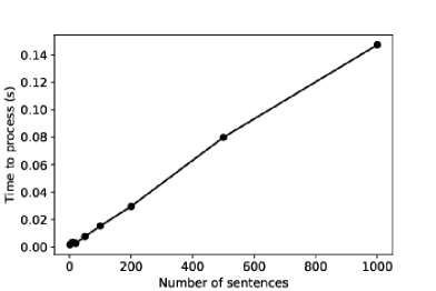
Figure 2: Processing time of the summarization function (y-axis) by the number of lines of the text as input (x-axis). Results computed on an i7-8550U.

5 Results

Tables 1 and 2 present the results for the CASS and the CNN/DailyMail datasets. As expected, the supervised model performs better than the unsupervised one. On the three datasets, the supervision has improved the score in terms of ROUGE-2 and ROUGE-L. In the same way, our oracles are always better than the learned models, proving that there is still room for improvements. Information concerning the length of the generated summaries and the position of the sentences taken are available in the appendices A.4.2.

On the French CASS dataset, our method performs similarly to the $rnn-ext$. The PGN performs a bit better (+0.13 ROUGE-1, +0.38 ROUGE-2, + 0.81 ROUGE-L compared to the other models), which could be linked to the fact that it can select elements smaller than sentences.

On the CNN/DailyMail dataset, our supervised model performs poorly. We observe a significant difference (+2.66 ROUGE-1, +3.38 ROUGE-2, and +4.00 ROUGE-L) between the two oracles. It could be explained by the fact that the summaries are multi-topic and our models do not handle such case. Therefore, as our loss doesn’t look at the diversity, STRASS may miss some topics in the generated summary.

A second limitation of our approach is that our model doesn’t consider the position of the sentences in the summary, information which presents a high relevance in the CNN-Dailymail dataset.

STRASS has some advantages. First, it is trainable on CPU and thus light to train and run. Indeed, the neural network in our model is only composed of one dense layer. The most recent advances in text summarization with neural networks are all based on deep neural networks requiring GPU to be learned efficiently. Second, the method is scalable. The processing time is linear with the number of lines of the documents (Figure 2). The model is fast at inference time as sent2vec embeddings are fast to generate. Our model generated the 13,095 summaries of the CASS dataset in less than 3 minutes on an i7-8550U CPU.

6 Conclusion and Perspectives

To conclude, we proposed here a simple, cost-effective and scalable extractive summarization method. STRASS creates an extractive summary by selecting the sentences with the closest embeddings to the projected document embedding. The model learns a transformation of the document embedding to maximize the similarity between the extractive summary and the ground truth summary. We showed that our approach obtains similar results than other extractive methods in an effective way.

There are several perspectives to our work. First, we would like to use the sentence embeddings as an input of our model, as this should increase the accuracy. Additionally, we want to investigate the effect of using other sent2vec embedding spaces (especially more generalist ones) or other embedding functions like doc2vec Le and Mikolov (2014) or BERT Devlin et al. (2019).

For now, we have only worked on sentences but this model can use any embeddings, so we could try to build summaries with smaller textual elements than sentences such as key-phrases, noun phrases… Likewise, to apply our model on multi-topic texts, we could try to create clusters of sentences, where each cluster is a topic, and then extract one sentence by cluster.

Moreover, currently, the loss of the system is only composed of the proximity and the compression ratio. Other meaningful metrics for document summarization such as diversity and representativity could be added into the loss. Especially, submodular functions could (1) allow to obtain near-optimal results and (2) allow to include elements like diversity Lin and Bilmes (2011). Another information we could add is the position of the sentences in the documents like Narayan et al. (2018a).

Finally, the approach could be extended to query-based summarization V.V.MuraliKrishna et al. (2013). One could use the embedding function on the query and take the sentences that are the closest to the embedding of the query.

Appendix A Appendices

A.1 Datasets

The composition of the datasets and the splits are available in table 3.

A.2 Preprocessing

On the French CASS dataset, we have deleted all the accents of the texts and we have lower-cased all the texts as some of them where entirely upper-cased without any accent. To create the summaries, all the ANA parts of the XML files provided in the original dataset where taken and concatenate to form a single summary for each document. These summaries explain different key points of the judgment. On the CNN/DailyMail, the preprocessing of See et al. (2017) was used. As an extra cleaning step, we deleted the documents that had an empty story.

A.3 Hyperparameters

To obtain the embeddings functions for both datasets we trained a sent2vec model of dimension 700 with unigrams on the train splits.

For the CASS dataset, the baseline model has a threshold at $0.8$, the oracle at $0.8$ and STRASS has a threshold at $0.8$ and a $\lambda$ at $0.3$. TextRank was used with a ratio of $0.2$. The PGN For the CNN/DailyMail dataset, the baseline model has a threshold at $1.0$, the oracle at $0.9$ and STRASS has a threshold at $0.8$ and a $\lambda$ at $0.4$. TextRank was used with a ratio of $0.15$.

A.4 Results

A.4.1 ROUGE Score

More detailed results are available in tables 4 and 5. High recall with low precision is generally synonym of long summary.

Dataset	$s_{d}$	$s_{s}$	$t_{d}$	$t_{s}$	train	val	test
CASS	19.4	1.6	894	114	103,434	12,916	13,095
CNN/DailyMail	28.9	3.8	786	53	287,112	13,367	11,489

Table 3: Size information for the datasets, $s_{d}$ and $s_{s}$ are respectively the average number of sentences in the document and in the summary, $t_{d}$ and $t_{t}$ are respectively the number of tokens in the document and in the summary. train, val and test are respectively the number of documents in the train, validation and test sets.

	R1 P	R1 R	R1 F1	R2 P	R2 R	R2 F1	RL P	RL R	RL F1
Baseline	32.27	65.81	39.55	17.98	36.88	22.09	24.13	50.11	29.69
TextRank	32.62	68.58	39.30	19.47	41.95	23.49	25.98	56.16	31.45
PGN	69.70	49.01	53.25	53.46	36.67	40.25	60.31	41.65	45.58
rnn-ext	49.54	69.62	53.12	35.94	50.00	38.30	42.03	58.43	44.77
STRASS	56.23	62.55	52.68	41.97	45.71	38.87	48.05	52.93	44.72
Oracle	66.40	68.41	62.79	53.80	53.40	50.10	58.73	59.20	55.03
Oracle sent	69.50	64.82	63.90	55.36	50.91	50.56	60.77	56.34	55.75

Table 4: Full results of different models on the French CASS dataset using ROUGE with 95% confidence. The models in the first part are unsupervised models, then supervised models and the last part is the oracle. P is precision, R is recall and F1 is the F-measure. R1, R2 and RL stand for ROUGE1, ROUGE2, and ROUGE-L.

	R1 P	R1 R	R1 F1	R2 P	R2 R	R2 F1	RL P	RL R	RL F1
Baseline	32.67	40.09	34.02	12.07	14.65	12.48	27.29	33.14	28.27
TextRank	23.44	59.29	30.83	9.95	25.02	13.02	20.77	53.02	27.39
PGN*			39.53			17.28			36.38
rnn-ext*			40.17			18.11			36.41
STRASS	28.56	53.53	33.99	11.89	22.62	14.18	25.21	47.46	30.04
Oracle	44.92	50.93	43.55	24.14	25.47	22.43	39.98	44.75	38.47
Oracle sent	35.17	74.30	46.21	19.84	40.83	25.81	32.37	68.12	42.47
Lead3	33.89	53.35	40.00	14.84	23.59	17.56	30.80	48.43	36.33
Lead - PGN*			40.34			17.70			36.57

Table 5: Full results of different models on the CNN/DailyMail. The Lead3 - PGN is the lead 3 score as reported in See et al. (2017). The scores with * are taken from the corresponding publications. P is precision, R is recall and F1 is the F-measure. R1, R2 and RL stand for ROUGE1, ROUGE2, and ROUGE-L.

Model	$s$	$w$	$w/s$
Reference	1.6	117	73.1
STRASS	2.0	151	75.5
Oracle	1.7	138	81.2
Oracle sent	1.5	112	74.7

(a) Size information for the generated summary on the test split of the CASS dataset, $s$, $w$, $w/s$ are respectively the average number of sentences, the average number of words and the average number of words per sentences.

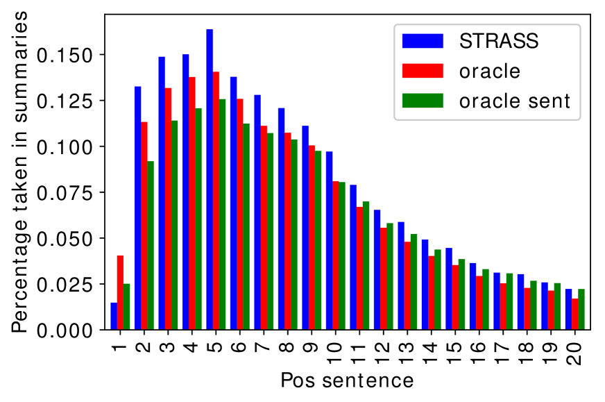
(a) Percentage of times that a sentence is taken in a generated summary in function of their position in the document on the CASS dataset.

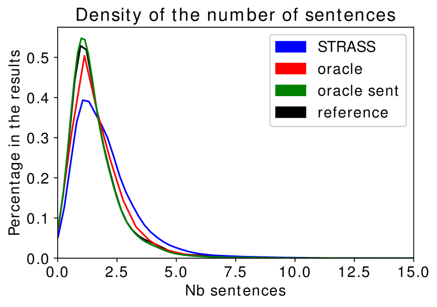
(b) Density of the number of sentences in the generated summaries for several models and the reference on the CASS dataset.

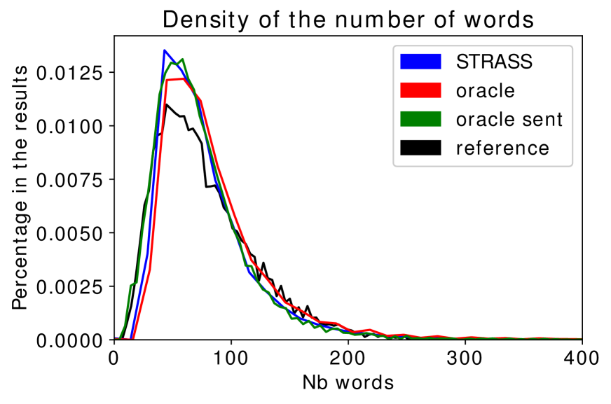
(c) Density of the number of words in the generated summaries for several models and the reference on the CASS dataset.

Figure 3: Information about the length of the generated summaries for the CASS dataset.

A.4.2 Words and sentences

On the French CASS dataset the summaries generated by the models are generally close in terms of length (number of words, number of sentences and number of words per sentences (figure 6(a), 3(b), 3(c))). All the tested extractive methods tend to select sentences at the beginning of the documents. The first sentence make an exception to that rule (figure 3(a)). We observe that this sentence can have the list of the lawyers and judges that were present at the case. STRASS tends to generate longer summaries with more sentences. The discrepancy in the average number of sentences between the reference and $Oraclesent$ is due to sentences that are extracted multiple times.

On the CNN/DailyMail dataset, STRASS tends to extract less sentences but longer ones comparing to the $Oraclesent$ (figure 7(a), 4(b), 4(c)). On the figure 4(a) we can see that the three models tend to extract different sentences. $Oraclesent$ which is the best performing model tends to extract the 4 first sentences, $Oracle$ extracts more often the fourth sentences than the first three and still have better results than the $Lead3$, which means that the fourth sentences could have some interest. With STRASS the first three sentences have a different tendency than the rest of the text, showing that the first three sentences may have a different structure than the rest. Then, the farther a sentence is in the text, the lower the probability to take it.

Model	$s$	$w$	$w/s$
Reference	3.9	55	14.1
STRASS	2.7	135	50
Oracle	1.5	84	56
Oracle sent	3.5	137	39.1

(a) Size information for the generated summary on the test split of the CNN/DM dataset, $s$, $w$, $w/s$ are respectively the average number of sentences, the average number of words and the average number of words per sentences.

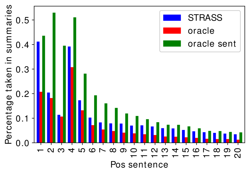
(a) Percentage of times that a sentence is taken in a generated summary in function of their position in the document on the CNN/DM dataset.

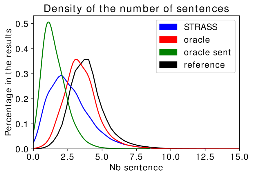
(b) Density of the number of sentences in the generated summaries for several models and the reference on the CNN/DM dataset.

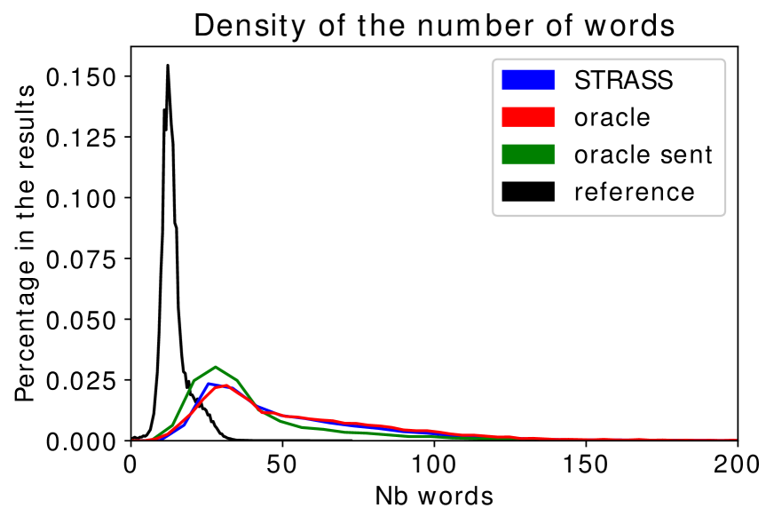
(c) Density of the number of words in the generated summaries for several models and the reference on the CNN/DM dataset.

Figure 4: Information about the length of the generated summaries for the CNN/DM dataset.

References

- Barrios et al. (2016) Federico Barrios, Federico López, Luis Argerich, and Rosa Wachenchauzer. 2016. Variations of the similarity function of textrank for automated summarization. CoRR, abs/1602.03606.
- Bennani-Smires et al. (2018) Kamil Bennani-Smires, Claudiu Musat, Andreea Hossmann, Michael Baeriswyl, and Martin Jaggi. 2018. Simple unsupervised keyphrase extraction using sentence embeddings. In Proceedings of the 22nd Conference on Computational Natural Language Learning, pages 221–229. Association for Computational Linguistics.
- Cao et al. (2018) Ziqiang Cao, Wenjie Li, Sujian Li, and Furu Wei. 2018. Retrieve, rerank and rewrite: Soft template based neural summarization. In Proceedings of the 56th Annual Meeting of the Association for Computational Linguistics (Volume 1: Long Papers), pages 152–161. Association for Computational Linguistics.
- Chen and Bansal (2018) Yen-Chun Chen and Mohit Bansal. 2018. Fast abstractive summarization with reinforce-selected sentence rewriting. In Proceedings of the 56th Annual Meeting of the Association for Computational Linguistics (Volume 1: Long Papers), pages 675–686. Association for Computational Linguistics.
- Denkowski and Lavie (2014) Michael Denkowski and Alon Lavie. 2014. Meteor universal: Language specific translation evaluation for any target language. In Proceedings of the Ninth Workshop on Statistical Machine Translation, pages 376–380. Association for Computational Linguistics.
- Devlin et al. (2019) Jacob Devlin, Ming-Wei Chang, Kenton Lee, and Kristina Toutanova. 2019. BERT: Pre-training of deep bidirectional transformers for language understanding. In Proceedings of the 2019 Conference of the North American Chapter of the Association for Computational Linguistics: Human Language Technologies, Volume 1 (Long and Short Papers), pages 4171–4186, Minneapolis, Minnesota. Association for Computational Linguistics.
- Hermann et al. (2015) Karl Moritz Hermann, Tomáš Kočiský, Edward Grefenstette, Lasse Espeholt, Will Kay, Mustafa Suleyman, and Phil Blunsom. 2015. Teaching machines to read and comprehend. In Proceedings of the 28th International Conference on Neural Information Processing Systems - Volume 1, NIPS’15, pages 1693–1701, Cambridge, MA, USA. MIT Press.
- Hsu et al. (2018) Wan-Ting Hsu, Chieh-Kai Lin, Ming-Ying Lee, Kerui Min, Jing Tang, and Min Sun. 2018. A unified model for extractive and abstractive summarization using inconsistency loss. In Proceedings of the 56th Annual Meeting of the Association for Computational Linguistics (Volume 1: Long Papers), pages 132–141. Association for Computational Linguistics.
- Le and Mikolov (2014) Quoc Le and Tomas Mikolov. 2014. Distributed representations of sentences and documents. In Proceedings of the 31st International Conference on Machine Learning, volume 32 of Proceedings of Machine Learning Research, pages 1188–1196, Bejing, China. PMLR.
- Lin (2004) Chin-Yew Lin. 2004. Rouge: A package for automatic evaluation of summaries. In Text Summarization Branches Out: Proceedings of the ACL-04 Workshop, pages 74–81, Barcelona, Spain. Association for Computational Linguistics.
- Lin and Bilmes (2011) Hui Lin and Jeff Bilmes. 2011. A class of submodular functions for document summarization. In Proceedings of the 49th Annual Meeting of the Association for Computational Linguistics: Human Language Technologies - Volume 1, HLT ’11, pages 510–520, Stroudsburg, PA, USA. Association for Computational Linguistics.
- Mihalcea and Tarau (2004) Rada Mihalcea and Paul Tarau. 2004. TextRank: Bringing order into text. In Proceedings of EMNLP 2004, pages 404–411, Barcelona, Spain. Association for Computational Linguistics.
- Mikolov et al. (2013a) Tomas Mikolov, Kai Chen, Greg Corrado, and Jeffrey Dean. 2013a. Efficient estimation of word representations in vector space. CoRR, abs/1301.3781.
- Mikolov et al. (2013b) Tomas Mikolov, Wen-tau Yih, and Geoffrey Zweig. 2013b. Linguistic regularities in continuous space word representations. In Proceedings of the 2013 Conference of the North American Chapter of the Association for Computational Linguistics: Human Language Technologies, pages 746–751, Atlanta, Georgia. Association for Computational Linguistics.
- Mori and Sasaki (2002) Tatsunori Mori and Takuro Sasaki. 2002. Information gain ratio meets maximal marginal relevance - a method of summarization for multiple documents. In NTCIR.
- Nallapati et al. (2016a) Ramesh Nallapati, Feifei Zhai, and Bowen Zhou. 2016a. Summarunner: A recurrent neural network based sequence model for extractive summarization of documents. CoRR, abs/1611.04230.
- Nallapati et al. (2016b) Ramesh Nallapati, Bowen Zhou, Cicero dos Santos, Caglar Gulcehre, and Bing Xiang. 2016b. Abstractive text summarization using sequence-to-sequence rnns and beyond. In Proceedings of The 20th SIGNLL Conference on Computational Natural Language Learning, pages 280–290, Berlin, Germany. Association for Computational Linguistics.
- Narayan et al. (2018a) Shashi Narayan, Shay B. Cohen, and Mirella Lapata. 2018a. Don’t give me the details, just the summary! topic-aware convolutional neural networks for extreme summarization. In Proceedings of the 2018 Conference on Empirical Methods in Natural Language Processing, pages 1797–1807, Brussels, Belgium. Association for Computational Linguistics.
- Narayan et al. (2018b) Shashi Narayan, Shay B. Cohen, and Mirella Lapata. 2018b. Ranking sentences for extractive summarization with reinforcement learning. In Proceedings of the 2018 Conference of the North American Chapter of the Association for Computational Linguistics: Human Language Technologies, Volume 1 (Long Papers), pages 1747–1759. Association for Computational Linguistics.
- Pagliardini et al. (2017) Matteo Pagliardini, Prakhar Gupta, and Martin Jaggi. 2017. Unsupervised learning of sentence embeddings using compositional n-gram features. CoRR, abs/1703.02507.
- Paulus et al. (2017) Romain Paulus, Caiming Xiong, and Richard Socher. 2017. A deep reinforced model for abstractive summarization. CoRR, abs/1705.04304.
- Rush et al. (2015) Alexander M. Rush, Sumit Chopra, and Jason Weston. 2015. A neural attention model for abstractive sentence summarization. In Proceedings of the 2015 Conference on Empirical Methods in Natural Language Processing, pages 379–389. Association for Computational Linguistics.
- See et al. (2017) Abigail See, Peter J. Liu, and Christopher D. Manning. 2017. Get to the point: Summarization with pointer-generator networks. In Proceedings of the 55th Annual Meeting of the Association for Computational Linguistics (Volume 1: Long Papers), pages 1073–1083. Association for Computational Linguistics.
- V.V.MuraliKrishna et al. (2013) R V.V.MuraliKrishna, S Y. Pavan Kumar, and Ch Reddy. 2013. A hybrid method for query based automatic summarization system. International Journal of Computer Applications, 68:39–43.