Equivariant fundamental classes in -graded cohomology with -coefficients
Abstract.
Let denote the cyclic group of order two. Given a manifold with a -action, we can consider its equivariant Bredon -graded cohomology. In this paper, we develop a theory of fundamental classes for equivariant submanifolds in -graded cohomology with constant coefficients. We show the cohomology of any -surface is generated by fundamental classes, and these classes can be used to easily compute the ring structure. To define fundamental classes we are led to study the cohomology of Thom spaces of equivariant vector bundles. In general the cohomology of the Thom space is not just a shift of the cohomology of the base space, but we show there are still elements that act as Thom classes, and cupping with these classes gives an isomorphism within a certain range.
1. Introduction
There has been recent interest in better understanding -graded Bredon cohomology. For example, explicit computations can be found in [CHT], [Ha], [Ho], [K2], [LFdS], and [Sh], and certain freeness and structure theorems can be found in [K1] and [M1]. In this paper, we consider -manifolds and develop a theory of fundamental classes for equivariant submanifolds in constant coefficients. These classes can be defined for both free and nonfree submanifolds. When two submanifolds intersect transversally, the cup product of their classes is given in terms of the fundamental class of their intersection. In order to define these classes, we consider equivariant Thom spaces for real -vector bundles and prove properties of the -graded cohomology of these spaces with constant coefficients.
To say more about the cohomology of Thom spaces, let denote the cohomology of a point with constant coefficients, and note the cohomology of any -space with -coefficients is an -module. We will show when the base is nonfree there is a unique class in a predicted grading that generates a free submodule and forgets to the singular Thom class. Cupping with this class gives an isomorphism from the cohomology of the base space to the cohomology of the Thom space within a certain range. When the base is free, we show there are infinitely many classes connected by a predicted module action that forget to the singular Thom class, and cupping with any one of these classes produces an isomorphism from the shifted cohomology of the base space to the cohomology of the Thom space.
The Thom classes for normal bundles allow us to define the previously mentioned fundamental classes. For nonfree submanifolds, there will be a unique fundamental class whose grading is determined by the normal bundle. For free submanifolds, there will be infinitely many fundamental classes all connected by a predicted module action. We will show the cohomology of any -surface is generated by fundamental classes of submanifolds, and that we can use these classes to easily compute the ring structure.
Let us begin by recalling some facts about Bredon cohomology; a more detailed exposition can be found in [HHR, Section 2], for example. For a finite group the Bredon cohomology of a -space is a sequence of abelian groups graded on , the Grothendieck group of finite-dimensional, real, orthogonal -representations. When is the cyclic group of order two, recall any -representation is isomorphic to a direct sum of trivial representations and sign representations. Thus is a free abelian group of rank two, and the Bredon cohomology of any -space can be regarded as a bigraded abelian group.
We will use the motivic notation for the Bredon cohomology of a -space with coefficients in a Mackey functor . The first grading indicates the dimension of the representation, and we will often refer to this grading as the “topological dimension”. The second grading indicates the number of sign representations appearing and will be referred to as the “weight”. Given any -space , there is always an equivariant map where denotes a single point with the trivial -action. This gives a map of bigraded abelian groups . If has the additional structure of a Green functor, then in fact this is a map of bigraded rings, and thus forms a bigraded algebra over the cohomology of a point. In this paper, we will be working with the constant Mackey functor , which is a Green functor, and we will write for the bigraded ring . In addition to being a Green functor, satisfies an additional property () that ensures is a bigraded commutative ring.
1.1. The cohomology of orbits
Since the cohomology of any -space with -coefficients is a bigraded module over a bigraded ring, we can use a grid to record information about the cohomology groups and module structures. The ring is illustrated on the left-hand grid in Figure 1 below. Each dot represents a copy of , and the connecting lines indicate properties of the ring structure. For example, the portion of the picture in quadrant one is polynomial in two elements and that have bidegrees and , respectively. The diagonal lines in the picture indicate multiplication by , while the vertical lines indicate multiplication by . A full description of can be found in Section 2. In practice, it is often easier to work with the abbreviated picture shown on the right-hand grid.
For the examples that follow, we also need the cohomology of the free orbit . We denote this -module by . Algebraically, , and in the figure below, we provide a detailed drawing of this module on the left and an abbreviated drawing on the right. The dots again indicate copies of while the vertical lines indicate action by .
1.2. Summary of main points
Now that we have established some notation, we provide a brief summary of the main goals of this paper. There are two main topics, fundamental classes and the cohomology of Thom spaces. These topics can be further divided into five subtopics:
-
(1)
Nonfree fundamental classes: Given a nonfree -manifold and a nonfree -submanifold , we prove there exists a fundamental class where and is found as follows. Consider the restriction of the equivariant normal bundle of in to the fixed set . Over each component of this fixed set, the fibers are -representations, and the isomorphism type of the representation is constant over each component. Thus each component corresponds to a representation of some weight, and the integer is chosen to be the maximum such weight.
-
(2)
Free fundamental classes: Given a -manifold (free or nonfree) and a free submanifold , we show there is an infinite family of classes where and is any integer. These classes satisfy the module relation .
-
(3)
Intersection product of fundamental classes: We show the cup product of two fundamental classes for nonfree submanifolds and that intersect transversally is given by a predicted -multiple of the fundamental class of the intersection. For free submanifolds, we show .
-
(4)
Restricted Thom isomorphism theorem for nonfree spaces: Let be a finite, nonfree -CW complex and be an -dimensional -vector bundle whose maximum weight representation over is . We show there is a unique class that restricts to -multiples of the generators of the cohomology of the fibers. We also show cupping with this class gives an isomorphism whenever .
-
(5)
Thom isomorphism theorem for free spaces: Let be a finite, free -CW complex. For an -dimensional -vector bundle , we show for each integer there is a unique class that restricts to the nonzero class in the cohomology of the fibers. In this case, cupping with any one of these Thom classes provides an isomorphism from the cohomology of the base space to the cohomology of a shift of the Thom space.
Remark 1.3.
These equivariant fundamental classes act in many ways just like their nonequivariant analogs, though, there are still various subtleties that arise in the equivariant context. For example, one might expect nonfree fundamental classes to always generate free summands and free fundamental classes to string together to form modules similar to . While this is often the case, there are exceptions. As shown in Example 1.9 below, there can be free submanifolds whose classes are nonzero for a while, but become zero in high enough weight. This and other subtleties are best explained through a series of examples.
1.4. Examples of equivariant fundamental classes
Before stating the general results, let’s consider some examples of -surfaces to determine what properties we might expect of equivariant fundamental classes.
Example 1.5.
We begin with a simple example. Let denote the -space whose underlying space is the genus one torus and whose -action is given by a reflection, as shown in Figure 3. The fixed set is shown in blue. As shown in the author’s previous work [Ha, Theorem 6.6], the cohomology of this space is given by
An abbreviated illustration of this module is given below.
Suppose we wanted to find equivariant submanifolds whose fundamental classes generate these free summands. Take, for example, the fixed circle labeled above. Topologically, this is a codimension one submanifold, so we would expect to have a fundamental class in bidegree for some , but how do we determine this value of ? Let’s consider a tubular neighborhood of . Note the tubular neighborhood is equivariantly homeomorphic to where denotes the sign representation, so one might expect a fundamental class in bidegree . Indeed, we will show there is such a class , and furthermore, this class generates a free summand in bidegree . We also have a class corresponding to the other fixed circle, and we will show .
Now consider the circle that travels around the hole of the torus and is isomorphic to a circle with a reflection action. In this case, the tubular neighborhood of is homeomorphic to where is the trivial representation. We expect to get a class in bidegree , and indeed such a class exists and generates a free summand.
These two circles intersect at a single fixed point whose tubular neighborhood is the unit disk in . The fundamental class generates a free summand in bidegree , and furthermore we obtain the relation
The submanifolds and do not intersect, so we also obtain the relation
We conclude
as an -algebra.
Remark 1.6.
In the example above, all of the considered submanifolds had trivial normal bundles, and this led to an obvious choice of bidegree for each fundamental class. Of course, we would like to have fundamental classes for submanifolds whose normal bundles are nontrivial. The next example illustrates this.
Example 1.7.
Let denote the -space given by the projective plane with action induced by the rotation action on the disk as shown in Figure 4. Again the fixed set is shown in blue. The cohomology of as an -module is given by
We again look for equivariant submanifolds. Consider the fixed circle labeled . The equivariant normal bundle is given by the nontrivial Möbius bundle over . This bundle is not trivial, but observe every point has an equivariant neighborhood such that . In other words, this bundle is a locally trivial -bundle, so we get a class .
Now consider the circle . This circle is isomorphic to a circle with a reflection action, and again the normal bundle is the nontrivial bundle over . Around the fixed point there is a neighborhood such that while around the point there is a neighborhood such that . The bundle is not a locally trivial -bundle for any -representation , so if it even exists, the bidegree of the fundamental class for is unclear.
We will show the fundamental class does exist, and its grading is determined by the fibers of the normal bundle over the fixed set. In this case, while . The class will have grading where is the maximum weight representation appearing over the fixed set, so in this case .
The classes and are both in bidegree , and we will see in Example 4.15 that . Let’s consider their product. One might hope
but something has gone wrong. The product has bidegree , while the fundamental class has bidegree . We will show a slightly modified formula holds. Namely
where recall . This gives us the relation
In Example 4.15 we use these classes to conclude as an -algebra
Remark 1.8.
The first two examples give a flavor of fundamental classes for nonfree submanifolds. It is natural to ask if such things can be defined for free submanifolds. We see this in the next example.
Example 1.9.
Let denote the -space whose underlying space is the genus two torus and whose -action is given by a rotation action with two fixed points, as illustrated below. The cohomology of this space is given by
In this example the cohomology is an infinitely generated, nonfree -module. The free submanifold is a codimension one submanifold, so we would expect to have a class . The submanifold is free, so there is no fixed set to determine the weight as in the previous examples. We will show there are actually infinitely many fundamental classes, one in each weight. That is, we have classes for all integers that are related via the formula
The submodule generated by these classes corresponds to a -summand. One can show the fundamental classes of the free submanifold generate the other summand. Lastly, there are classes corresponding to the two fixed points. Either class will generate a free summand in bidegree , and the classes are related via .
We can also choose a point and consider the classes . One might expect these classes to all be zero, but in fact, they are nonzero whenever . The intersection product then leads to some interesting relations as shown in Example 4.18.
We mention two other nonfree classes one might consider. There are two copies of a circle with a reflection action in the space . We can consider the circle that travels around the equator through and , and the circle that travels around the perimeter of the picture through and . Call these circles and , respectively. Then while .
1.10. Nonequivariant fundamental classes
Before trying to define equivariant fundamental classes, let’s recall nonequivariant fundamental classes. Let be a closed manifold and be a closed, connected submanifold of codimension . We can define the fundamental class using the classical Thom isomorphism theorem from [T].
Consider the normal bundle of in . Let be a tubular neighborhood of . By excision
By the Thom isomorphism theorem, the righthand group is and generated by the Thom class . Thus there exists a unique nonzero class in . We now define the fundamental class to be the image of this unique class under the induced map from the inclusion of the pairs . Recall these classes have a nice intersection product. If and are two submanifolds of that intersect transversally, then .
One goal of this paper is to define an equivariant analog to these classes in Bredon cohomology. Given an equivariant submanifold, the above hints that we should consider the normal bundle, and use some fact about the cohomology of the corresponding Thom space. Unfortunately, no direct analog of the Thom isomorphism theorem exists for general -vector bundles in -coefficients; see Example 3.4 for an example of a vector bundle such that the cohomology of is not just a shift of the cohomology base space. Despite this failure, we can still prove a weaker version of the Thom isomorphism theorem, and this is enough to define fundamental classes.
1.11. The main theorems
We now state the main results of this paper. In what follows, let denote the -module . It was shown in [M2, Theorem 5.1] that as a module over the cohomology of a point, the cohomology of any finite -CW complex is isomorphic to a direct sum of free modules and shifted copies of for various values of .
We begin with nonfree -vector bundles. Let be a finite, nonfree -CW complex and let be a real -dimensional -vector bundle (precise definitions can be found in Section 3). Let denote the connected components of the fixed set . As explained in Section 3, there exist weights ,…, such that for all , the fiber . Let be the maximum such weight. We will prove the following where all coefficients are understood to be .
Theorem 1.12.
Let , , , , and be defined as above and let . There exists a unique class that restricts to the nonzero class over both free and nonfree fibers. Furthermore this class satisfies the following properties:
-
(i)
is the singular Thom class, where is the forgetful map;
-
(ii)
, where denotes the submodule generated by ;
-
(iii)
If is nonfree, then for , we have the naturality formula for a determined value of ;
-
(iv)
Under the inclusion of fixed points , we have that where ;
-
(v)
The map is an isomorphism if ;
-
(vi)
Suppose Then where the weights satisfy ;
-
(vii)
If in fact for all , then is an isomorphism in all bidegrees and
Let be a nonfree -codimensional equivariant submanifold of and let denote the equivariant normal bundle. We can construct an equivariant tubular neighborhood of , and then use the class to get a class . As with the nonequivariant classes, we have a nice formula for how these classes multiply. For now, we state a summary. Recall .
Theorem 1.13.
Let be a nonfree, -dimensional -manifold, and let and be two closed, nonfree equivariant submanifolds. Suppose intersects transversally in the nonequivariant sense and that is a nonfree submanifold. Then there is a unique integer such that
The exact value of is dependent on , , and and is given explicitly in Theorem 4.10.
For free -vector bundles, we will prove something similar. Again the coefficients are understood to be .
Theorem 1.14.
Let be a free, finite -CW complex and let be a real -vector bundle and . For every integer there exists a unique class that restricts to the nonzero class over fibers. Furthermore this class satisfies the following properties:
-
(i)
is the singular Thom class, where is the forgetful map;
-
(ii)
;
-
(iii)
If is free, then for , we have the naturality formula ;
-
(iv)
The map is an isomorphism for all . In particular, .
Now given a free submanifold, we can use the classes corresponding to the normal bundle to define fundamental classes for all . There is also a nice intersection product for these free fundamental classes.
Theorem 1.15.
Let be an -dimensional -manifold, and suppose and are equivariant submanifolds that intersect transversally in the nonequivariant sense and whose intersection is free. We have the following cases for the product of their fundamental classes.
-
•
Suppose and are nonfree and their fundamental classes have weights , , respectively. Then
-
•
Suppose is nonfree and is free. Then for every ,
-
•
Suppose and are both free. Then for every , ,
In the last section of this paper, we show these classes give a geometric interpretation for the Bredon cohomology of -surfaces. Specifically, we prove the following theorem.
Theorem 1.16.
As an -module, the Bredon cohomology of any -surface is generated by fundamental classes of submanifolds.
Remark 1.17.
There are many examples of -surfaces whose Bredon cohomology is infinitely generated as an -module; see Example 1.9. This is unsurprising given that the modules are infinitely generated. Though, there is always a finite list of submanifolds whose fundamental classes generate the cohomology, and any free -summand is generated by fundamental classes of free submanifolds.
1.18. Organization of the paper
There are two main topics in this paper, fundamental classes and the cohomology of Thom spaces. We define fundamental classes using Thom classes of normal bundles, so the topics are certainly related, but the full discussion of one is not required for the other. Section 2 reviews relevant information about Bredon cohomology that is needed for either topic. After that, Section 3 discusses Thom classes and the cohomology of Thom spaces. Section 4 defines fundamental classes using the main theorems in Section 3. In Section 5 we provide the necessary background on -surfaces in order to then prove Theorem 1.16 in Section 6. Finally Appendix A contains a technical algebraic proof needed to prove property (vi) of Theorem 1.12.
1.19. Acknowledgements
The work in this paper was part of the author’s thesis project at University of Oregon. The author would like to thank her doctoral advisor Dan Dugger for all of his guidance and for many helpful conversations. The author would also like to thank Robert Lipshitz for his support. Lastly many thanks to the anonymous referee for their careful reading of this paper and for their helpful advice.
2. Background on Bredon cohomology
In this section, we review some preliminary facts about -graded Bredon cohomology when . While we regard this theory as graded on , it should be noted Bredon cohomology is not canonically graded on , and in general, one should be careful when working with these theories. These grading issues do not arise in this paper, so we do not expand on that point here; instead see [M2, Chapters IX.5 and XIII.1] for a more careful discussion of the grading.
2.1. Mackey functors
The coefficients of any -graded Bredon cohomology theory are what is known as a Mackey functor. In general, the definition of a Mackey functor requires some work, and a general exposition of Mackey functors can be found in Shulman’s thesis [Sh, Section 2.2] and in May’s book [M2, Chapter IX.4]. In the case of , the definition can be distilled to the following.
Definition 2.2.
A Mackey functor for is the data of
where and are abelian groups, and , , are homomorphisms that satisfy
-
(i)
,
-
(ii)
,
-
(iii)
, and
-
(iv)
.
Given an abelian group , we can form the constant Mackey functor where , , , and . We will be concerned with the following constant Mackey functor:
2.3. Bigraded theory
For a group , Bredon cohomology is graded on , the Grothendieck ring of finite-dimensional, real, orthogonal -representations. When is the cyclic group of order two, any such -representation is isomorphic to a direct sum of copies of the trivial representation and copies of the sign representation . Up to isomorphism, is entirely determined by its dimension and the number of sign representations appearing in this decomposition. It follows that is a rank free abelian group with generators given by and . For brevity, we will write for the representation . We will also write for the element of that is equal to . For the cohomology groups, we will write for the cohomology group .
Given any finite-dimensional, real, orthogonal, -representation we can form the one-point compactification . This new space will be an equivariant sphere which we will denote ; such spaces are referred to as representation spheres. Using these representation spheres, we can form equivariant suspensions. Whenever we have a based -space , we can form the -th suspension of by
Note the basepoint must be a fixed point. Often when working with free spaces we will add a disjoint basepoint in order to form suspensions and cofiber sequences. We use the common notation of for where the disjoint basepoint is understood to be fixed by the action.
An important feature of Bredon cohomology is that we have suspension isomorphisms: given any finite dimensional, real, orthogonal -representation, there are natural isomorphisms
Given a cofiber sequence of based -spaces
we can form the Puppe sequence
where is the one-dimensional trivial representation. From the suspension isomorphism this yields a long exact sequence
for each representation .
When , we have already discussed how the Bredon cohomology theory is a bigraded theory, and we will carry this notation over when discussing representation spheres and equivariant suspensions. In particular, we will denote by and for a based space we will denote by . Translating the above into this notation, we have natural isomorphisms
for all . Given a cofiber sequence we have long exact sequences
for each .
Three particular representation spheres will appear often in this paper, namely , , and . We include an illustration of these equivariant spheres in Figure 6. The fixed set is shown in blue while the arrow is used to indicate the action of on the space.
2.4. The cohomology of orbits
Given any -space we have an equivariant map where denotes a single point with the trivial action. On cohomology, this gives a map of rings . Thus the cohomology of is a module over the cohomology of a point, which we denote . Below we describe the cohomology of as well as the cohomology of the free orbit . These computations have been done many times, and are often attributed to unpublished notes of Stong. The computation for coefficients in any constant Mackey functor can be found in work of Lewis [L, Section 2]. A computation for constant integer coefficients can also be found in work of Dugger [D1, Appendix B], and the same methods used there can be used to compute the cohomology of orbits in constant coefficients.
In -coefficients, the cohomology of a point is given by the trivial square zero extension
where , , and . This ring is illustrated in the left-hand grid shown in Figure 7. The spot on the grid refers to the -cohomology group. Each dot represents a copy of , and we adopt the convention that the group is plotted up and to right of the coordinate. For example, is isomorphic to , while is zero.
We will often refer to portion of the cohomology in the first quadrant as the top cone and refer to the other portion as the bottom cone. The top cone is polynomial in the elements and . Multiplication by is indicated with vertical lines, and multiplication by is indicated with diagonal lines. The nonzero element in bidegree is divisible by all non-zero elements in the top cone.
In practice, it is often easier to work with an abbreviated picture, which is given on the right-hand grid in the above figure. It is understood that there is a at each spot within the top cone and within the bottom cone with the relations described above.
Note we now know the cohomology of all representation spheres by the suspension isomorphism. Specifically,
where denotes the free -module generated in bidegree . Visually, we just shift the picture units.
We also include the cohomology of the free orbit . As a ring, is isomorphic to where is in bidegree . As an -module, is isomorphic to . See Figure 8 for the pictorial representation of this module and its abbreviated version. In these module pictures, action by is indicated by vertical lines, while action by is indicated by diagonal lines.
2.5. Cohomology of the antipodal spheres
We review the cohomology of another family of spheres. The importance of these spaces will be clear shortly. Let denote the equivariant -sphere whose -action is given by the antipodal map. The cohomology of the antipodal spheres is given by
as an -module. This result is well known, but a detailed computation can be found in [Ha, Example 3.4]. The module can be represented pictorially as shown in Figure 9.
2.6. Some helpful theorems
We conclude this section by collecting some helpful lemmas and theorems that will be used in the paper. Many of the statements involve finite -CW complexes, so we first provide a definition of such spaces.
Definition 2.7.
A -CW complex is a -space with a filtration such that consists of a disjoint union of orbits and , and such that is obtained from by attaching cells of the form for or via the usual pushout diagram:
We begin with a lemma that relates the singular cohomology, the Bredon cohomology, and the action of . This statement follows from considering the long exact sequence associated to and is originally due to [AM].
Lemma 2.8.
(The forgetful long exact sequence). Let be a pointed -space. For every integer , we have a long exact sequence
where the coefficients are understood to be .
We will refer to the map as the “forgetful map”. Note in , the element forgets to , while forgets to zero. Indeed, by the exactness of the forgetful long exact sequence, for any , a given cohomology class forgets to zero if and only if it is the image of .
There are two types of spaces we will encounter in this paper whose cohomology is entirely dependent on the singular cohomology. These lemmas are likely well-known, but a recent proof in the same notation can be found in [Ha, Section 3].
Lemma 2.9.
Let be a trivial finite -CW complex. Then as -modules
Lemma 2.10.
Let be a finite -CW complex. The cohomology as an -module of the free -space is given by
Remark 2.11.
We next mention an important theorem about the cohomology of -manifolds. Here by “-manifold” we mean a piecewise linear manifold with a locally linear -action. By closed, we simply mean a closed manifold in the nonequivariant sense. The proof of this theorem is given in [Ha, Appendix A].
Theorem 2.12.
Let be an -dimensional, closed -manifold with a nonfree -action. Suppose is the largest dimension of submanifold appearing as a component of the fixed set. Then there is exactly one summand of of the form where , and it occurs for .
We conclude this section by recalling a structure theorem for the cohomology of finite -CW complexes proven in [M1, Theorem 5.1]. Note it is important that is finite in the sense that it contains only finitely many cells.
Theorem 2.13 ([M2]).
For any finite -CW complex , we can decompose the -graded cohomology of with constant -coefficients as
as a module over where denotes the cohomology of the -sphere with the free antipodal action. Furthermore, the shifts are given by actual representations. That is, for all and for all .
When is free or has only one fixed point, we get a refined structure theorem that follows from the isomorphism discussed in Remark 2.11.
Corollary 2.14.
If is a free finite -CW complex, then
Similarly if is a finite -CW complex with exactly one fixed point, then
Lastly we record a corollary of Theorem 2.13 that will be helpful later on.
Lemma 2.15.
Let be a finite -CW complex. For , action by gives an isomorphism if .
Proof.
By inspection this holds for modules of the form and where . The statement then follows from Theorem 2.13. ∎
3. -vector bundles and Thom isomorphism theorems
In this section, we provide some background on -vector bundles and then prove the Thom isomorphism theorems given as Theorem 1.12 and Theorem 1.14 in the introduction. Another approach to the Thom isomorphism is given in [CW] and uses a grading system larger than the usual -grading. Presumably there is a connection between the two approaches, but we haven’t investigated this.
We begin by reviewing -vector bundles. The following can be found in [Se, Section 1].
Definition 3.1.
Let be a -space. A -vector bundle over is the data of a nonequivariant vector bundle such that is a -space. Furthermore, should act on via vector bundle maps over the action of on . Explicitly, the following diagram should commute where denotes the action of ,
and for each the restriction of the action to the fibers
should be a linear map.
Many of the constructions for nonequivariant bundles exist for -vector bundles. For example, if the base space is paracompact and Hausdorff, then any -vector bundle can be given a -invariant Euclidean metric that allows us to define the unit disk bundle and the unit sphere bundle, which in turn allows us to define the Thom space. Also, given an equivariant map and a vector bundle we can form the pullback bundle . When working with these pullback bundles, the following important fact is still true; see [Se, Proposition 1.3] for a proof.
Lemma 3.2.
Let and be -CW complexes. Suppose are equivariantly homotopic and is a -vector bundle. Then as -vector bundles over .
The following lemma follows immediately from the above.
Lemma 3.3.
Let be a finite dimensional -vector bundle over a -CW complex. Suppose are two fixed points contained in the same connected component of . Then the fibers and are isomorphic as -representations.
While many of the constructions and basic lemmas carry over from nonequivariant vector bundle theory, issues arise when we start considering cohomology. In particular, there is no direct analog of the Thom isomorphism theorem in Bredon cohomology that holds for general vector bundles in -coefficients, as seen in the following example.
Example 3.4.
Let be the nontrivial one-dimensional bundle over . An illustration of the disk bundle is shown below. As usual, the fixed set is shown in blue, while conjugate points are indicated by matching symbols.
In this example, there are two components of the fixed set of the base space, both of which are isolated points. Over one point, the fiber is isomorphic to the -representation ; over the other point, the fiber is isomorphic to the -representation . We have
where and are the unit disk and unit sphere bundle, respectively. Now is a familiar space: the underlying space is the projective plane, so in particular, it is a -surface with exactly one fixed circle and one fixed point. The cohomology is given by Theorem 5.9 to be
On the other hand, the cohomology of the base space is given by the suspension isomorphism to be
We see the cohomology of the Thom space is not a shift of the cohomology of the base space, but there are still similarities. There are the same number of free summands, and both summands are shifted by one topological dimension. There is also a unique class in that generates a free summand and has topological dimension equal to the dimension of the bundle. Note the weight of this class corresponds to the maximum weight representation over the fixed set. This class will be the Thom class described in Theorem 3.16.
3.5. The Thom isomorphism in bigraded Borel cohomology
Before considering Bredon cohomology, we first analyze the Borel equivariant cohomology of -equivariant Thom spaces. This analysis will prove useful in our proof of the Thom isomorphism in Bredon cohomology.
Notation 3.6.
In the remainder of this section, all coefficients will be understood to be . Given a vector bundle over a space , we will write for the complement of the zero section and for the Thom space.
We begin by recalling the definition of Borel cohomology. As usual denotes a contractible -space with a free -action. For example, one can take with the antipodal action.
Definition 3.7.
Let be a -space. The bigraded Borel cohomology of is given by . The reduced bigraded Borel cohomology of a pointed -space is given by
The Borel cohomology of the orbits is given in the lemma below. The computation is straight-forward from the definition, so we leave the proof to the reader.
Lemma 3.8.
As a ring where and . As a -algebra, with acting as zero.
Remark 3.9.
The quotient lemma implies
so the bigraded Borel cohomology is indeed an extension of the usual Borel cohomology when working with constant coefficients. In fact, the bigraded Borel cohomology is entirely determined by the singly-graded Borel cohomology, as explained in the lemma below.
Lemma 3.10.
Let be a finite -CW complex and let denote the polynomial generator of . Then
where the module structure on the right factor is given by .
Proof.
Observe is a flat -module, so
is a bigraded cohomology theory for finite complexes. Now and we have a natural map
given by . One can check this gives an isomorphism when and , and thus the above is an isomorphism whenever is a finite -CW complex. ∎
Remark 3.11.
If is free, then the projection map is a weak equivalence of -spaces. Hence the Bredon cohomology and the Borel cohomology are isomorphic. Since in the free case, this gives the isomorphism mentioned in Remark 2.11.
We now prove there is a Thom isomorphism theorem for Borel cohomology. Let be an -dimensional -vector bundle. In the theorem below denotes the fiber for a fixed point , and denotes the fiber for conjugate points . Note for some weight while . On cohomology
Theorem 3.12.
Let be a finite -CW complex and let be an -dimensional -vector bundle. Then there is a unique class that satisfies the following properties:
-
(i)
The class restricts to the unique nonzero class over both free and nonfree fibers. That is, if then under the inclusion the class is the nonzero element in . Similarly if then under the inclusion , the class is the unique nonzero class in ;
-
(ii)
The map is an isomorphism.
Proof.
The singly graded Borel cohomology is defined using singular cohomology, so our strategy is to apply the singular cohomology Thom isomorphism theorem to get the corresponding theorem for Borel cohomology. We do this by making the following observation: if is a free -space and is a -vector bundle, then is also a vector bundle (this is discussed in the proof of [Se, Proposition 2.1], for example).
Consider the bundle . Applying the above observation, we have a vector bundle . The usual Thom isomorphism theorem gives a class
and the map
is an isomorphism. The domain is exactly and for the codomain, there is a homeomorphism of spaces
given by . Let . We have the following isomorphisms:
Since acts invertibly on the Borel cohomology, it follows that the bottom isomorphism holds for any weight, not just zero. Lastly the statements about restricting to fibers follow because these statements hold for . ∎
3.13. The Thom isomorphism in Bredon cohomology for trivial spaces
We next consider -vector bundles where the base space has a trivial -action. In this case, there is a Thom isomorphism theorem for Bredon cohomology that can be proven using the same methods as the singular Thom isomorphism theorem.
Lemma 3.14.
Suppose is a finite, connected -CW complex with a trivial -action and is a -vector bundle. Suppose the fiber over some point is isomorphic to . Then there is a unique class such that restricts to the nonzero class over fibers. Furthermore, the class satisfies the following properties:
-
(i)
The map is an isomorphism; and
-
(ii)
If is another trivial -CW complex and there is a map , then .
Proof.
The proof of this theorem is analogous to the proof of the usual Thom isomorphism for finite CW complexes, so we only provide an outline. Using compactness, we can cover with finitely many neighborhoods such that . For trivial bundles, the existence of a Thom class follows from the suspension isomorphism. We can now paste these classes together using the Mayer-Vietoris sequence, just as in the proof of the nonequivariant Thom isomorphism theorem. Property (i) then follows from the five-lemma, and property (ii) follows by restricting to fibers and using the uniqueness of the Thom class. ∎
3.15. The Thom isomorphism theorem for Bredon cohomology
We are now ready to prove the main theorems of this section. Our goal is to prove there exist Thom classes in Bredon cohomology for -vector bundles over finite -CW complexes and that these classes satisfy a list of properties. The two theorems are stated separately for nonfree versus free base spaces and are each broken into two parts. We begin with some setup for the nonfree case.
Let be a finite, nonfree -CW complex and be an -dimensional -vector bundle. Let denote the connected components of the fixed set . By Lemma 3.3, for each there is an integer such that for all , . Let . We now state the first part of the theorems.
Theorem 3.16 (Thom isomorphism for nonfree base spaces, Part I).
Let , , , , and be defined as above and let . There exists a unique class such that the following holds:
-
(i)
For every and , the class restricts to where is the generator of ;
-
(ii)
For every , the class restricts to the unique nonzero class in bidegree (n,q) in where ;
-
(iii)
The map is an isomorphism in bidegrees whenever ; and
-
(iv)
If in fact for all , then is an isomorphism in all bidegrees and .
Theorem 3.17 (Thom isomorphism for free base spaces, Part I).
Let be a free -space and be an -dimensional -vector bundle. Then for each there is a unique class such that the following holds:
-
(i)
For every pair of conjugate points , the class restricts to the unique nonzero element in bidegree in ;
-
(ii)
; and
-
(iii)
The map is an isomorphism for all ;
Proof of Theorem 3.16 and Theorem 3.17.
The proof will use Theorem 3.12, Theorem 3.14, and the following homotopy pushout square:
| (3.17.1) |
One can check this is a homotopy pushout square by considering the maps on the underlying spaces and then on the fixed sets. Using the square above, we get the following long exact sequence from applying reduced Bredon cohomology:
By definition, the Bredon cohomology of is the bigraded Borel cohomology of . By Theorem 3.12 there is a Thom class . We can multiply this class by powers of to get elements . Note acts invertibly on Borel cohomology, so satisfies the same properties as .
If is free, then is empty and . The map is surjective and by restricting to fibers, one can check the Thom class is sent to zero. Thus is injective and there is a unique lift of . Let be the pullback of under this isomorphism. Note if , we can still make sense of this because acts invertibly on Borel cohomology. The class then satisfies the properties of the theorem due to the properties of . This completes the proof of Theorem 3.17.
If is nonfree, then we need to consider . Recall are the connected components of . Let be the restriction of to . Then and
Each component is a connected and finite CW-complex, so we can apply Lemma 3.14 to get Thom classes . Let where recall is the largest of the .
Roughly speaking, we now paste together the classes and to get the class described in Theorem 3.16. To be more precise, let’s consider the following portion of the long exact sequence described at the beginning of the proof:
By the Borel Thom isomorphism theorem,
These groups aren’t zero when working unreduced because the cohomology of a point is , but the map will be an isomorphism (this is just the cohomology of a point mapping to itself). Thus the left map in the above sequence must be zero and the right map is injective. Let’s extend the long exact sequence to the right to get the following:
We next show maps to zero under the right map by restricting to the fibers. Let and let denote the one-point compactification of the fiber . We have a homotopy pushout square as shown below, and the inclusion gives a map from the square below to the square shown in 3.17.1.
| (3.17.2) |
Let’s consider the long exact sequence for the above square as well as the induced map to square shown in 3.17.1. We get the following commutative square:
| (3.17.3) |
The sum of the restrictions of and maps to zero in the down-across route (this can be seen by forgetting to singular cohomology, for example), and thus maps to zero in the top row. We can now define the class in to be the unique pullback of this sum.
To finish the proof, we just need to check satisfies the various properties described in the theorem. Most of these properties follow immediately from properties of and . For property (i), consider the diagram labeled 3.17.3. Note where is the generator of . If we extend the rows of this diagram to the left, then we see under the restriction as well. We can similarly show property (ii) by considering the fibers and using . To prove property (iii), we consider the following map of long exact sequences:
By the five-lemma, the center vertical map will be an isomorphism if the previous two and following two vertical maps are isomorphisms. Multiplication by the Borel Thom class always gives an isomorphism, but issues arise when considering . Recall the class was defined to be the sum and does not act invertibly on . Though, the map given by multiplication by is an isomorphism whenever by Lemma 2.15. Note if , then , so we can apply the five lemma to see multiplication by is an isomorphism whenever . This proves property (iii). If for all i, then cupping with is an isomorphism in all ranges, and this gives property (iv). This completes the proof of Theorem 3.16. ∎
Part I of the theorems proved the defining properties of Thom classes in Bredon cohomology. In the second part we prove additional properties of the Thom classes and of the cohomology of Thom spaces.
Theorem 3.18 (Thom isomorphism for nonfree base spaces, Part II).
Let , , , , , and be defined as in Theorem 3.16. The following additional properties hold:
-
(v)
is the singular Thom class, where is the forgetful map;
-
(vi)
where denotes the submodule generated by ;
-
(vii)
Suppose
Then
where the weights satisfy .
Proof.
For properties (v) and (vi), let such that . By restricting to this fiber and forgetting to singular cohomology, we get the following commutative diagram:
The top horizontal map takes to the generator, and thus is nonzero. This holds for all fibers, and so it must be that is the singular Thom class; this shows property (v). For (vi), note must be nonzero because of the top map. In [M1, Lemma 4.1], it is shown the class detects copies of , which proves property (vi).
All that remains is property (vii). This property relies on a somewhat technical proof about “nice” -modules. This is given in Appendix A. ∎
Theorem 3.19 (Thom isomorphism for free base spaces, Part II).
Let , , and be defined as in Theorem 3.17. The following additional properties hold:
-
(iv)
is the singular Thom class, where is the forgetful map; and
-
(v)
For any -CW complex and map , .
Proof.
Property (iv) can be proven just as property (v) in the previous theorem. For property (v), note must also be free, and then the statement follows by restricting to fibers and using uniqueness of the Thom class for bundles over free -CW complexes. ∎
There is also a naturality statement for maps to nonfree -CW complexes. We include this as a proposition below.
Proposition 3.20 (Naturality of nonfree Thom class).
Let and be finite -CW complexes and suppose is nonfree. Let be an -dimensional -vector with maximum weight over . For any map , there are two cases for :
-
(i)
If is free, then ; and
-
(ii)
If is nonfree, then where is the maximum weight of fibers over in (note ).
Proof.
These statements follow by restricting to fibers and using the uniqueness of the Thom class. ∎
We conclude this section by considering what happens to the nonfree Bredon Thom class under taking fixed points; this will be helpful in our discussion of fundamental classes that follows. Suppose is nonfree and as before, let be the connected components of . Again suppose we have an -dimensional -vector bundle such that the weight of the fibers over each is . By taking fixed points of , we obtain a vector bundle of dimension . The inclusion induces a map
Proposition 3.21.
Under the map where is the map described above, we have .
Proof.
Let and consider the restriction to this fiber and the restriction to the fixed sets. Note and these restrictions fit together to give the following commutative diagram:
Let and denote the respective generators of these rank one free modules. Let’s analyze the bottom right map. Consider the cofiber sequence . If the bottom horizontal map was zero, the associated long exact sequence to this cofiber sequence would imply is a rank two free module, but the space has exactly one fixed point, so this contradicts Corollary 2.14. Thus the bottom horizontal map is not zero and it must be that .
To prove the proposition, we trace the Thom class around the diagram. Under the left diagonal map , which then under the bottom horizontal map goes to . Under the upper left horizontal map by construction. Thus must map to a class in that restricts to . Since this must hold over every component, the only such class is . The composition of the upper horizontal maps is exactly , so this completes the proof. ∎
4. Fundamental classes
We now employ Theorems 3.16 and 3.17 to define fundamental classes for -submanifolds. We prove a handful of properties about these classes, such as how they forget to the usual singular fundamental classes, and how the product of these fundamental classes is given in terms of the intersection of the submanifolds in the transverse case. We end the section with a series of examples.
4.1. Nonequivariant fundamental classes
Recall for singular cohomology, we can define fundamental classes using the Thom isomorphism theorem as follows. Let be a closed -dimensional manifold and be a closed -dimensional submanifold. If we are working with -coefficients, all vector bundles over are orientable. In particular, if is the normal bundle of in , then the Thom isomorphism theorem guarantees a unique class known as the Thom class and
is an isomorphism. There exists a tubular neighborhood of in , and by excision we have the following isomorphism
Thus there is a unique nonzero class in corresponding to the Thom class. We can now define to be the image of this unique class under the induced map from the inclusion of pairs . We will often denote these singular classes by to distinguish them from the Bredon cohomology fundamental classes defined below.
4.2. Definitions and first properties
In Section 3, we proved properties of the cohomology of Thom spaces of -vector bundles. These properties are enough to transfer the above definition from the singular world to the equivariant world.
Let be a closed -manifold and be a closed -submanifold. First suppose both and are nonfree, and suppose topologically is -dimensional and is -dimensional. Let be the normal bundle of in , and let be the maximum weight of over as in Theorem 3.16. By this theorem, we are guaranteed a unique class . Let be an equivariant tubular neighborhood of . Using this neighborhood and excision
We are now ready for the following definition.
Definition 4.3.
Let , , , , and be defined as above. The unique nonzero class in corresponding to the Thom class in the above isomorphism is denoted by and referred to as the relative fundamental class of in . The image of this class in under the induced map by the inclusion of the pair will be denoted and referred to as the fundamental class of in .
The following corollary of property (v) of Theorem 3.18 relates these equivariant fundamental classes to the nonequivariant fundamental classes.
Corollary 4.4.
Suppose as above. Then where is the forgetful map to singular cohomology.
For , let where each is a connected component. We have the following corollary to Proposition 3.21.
Corollary 4.5.
Under the map , .
We can similarly define fundamental classes for free submanifolds. Let be an -dimensional -manifold and be a -dimensional -submanifold with a free -action. Again we can consider the normal bundle and from Theorem 3.17, we have the Thom class for each weight . We can now define the following.
Definition 4.6.
Let , , , , and be as above. For every integer , the unique element in corresponding to the Thom class is denoted and referred to as the relative fundamental class of in of weight . The image of this relative class under the map induced by the inclusion of pairs is denoted and referred to as the fundamental class of in of weight .
Corollary 4.7.
Suppose as above. Then and where is the forgetful map to singular cohomology.
4.8. Naturality and product formulas
We now prove there are naturality and intersection product formulas for equivariant fundamental classes. The first theorem is a consequence of property (ii) of Theorem 3.17 and Lemma 3.20.
Theorem 4.9 (Naturality of fundamental classes).
Let and be -manifolds and be a -submanifold of topological codimension . Suppose is a smooth map that is transverse to . Then we have the following pullback formulas:
-
(i)
If is free and is nonfree with , then ;
-
(ii)
If is nonfree with and is nonfree with , then ; and
-
(iii)
If and are free, then for all .
Proof.
Let . Denote the normal bundle for in by and the normal bundle for in by . For each the derivative of gives a map of tangent spaces . By definition of transversality, . Thus we get a map on the quotient which gives a map of bundles . We have the following commutative square
which implies there is a map to the pullback . This is an isomorphism on all fibers and thus an isomorphism of vector bundles.
Let denote the Pontryagin-Thom collapse map. An equivalent way to define the fundamental class of is to pull back the Thom class for under . Similarly we can define the fundamental class of using . We have the following commutative diagram in the homotopy category:
Consider cases (i), (ii), and (iii) in the theorem. The commutativity of the right triangle along with Lemma 3.20 imply in case (i) and in case (ii) . Part (iv) of Theorem 3.19 implies in case (iii) . Pulling back to and then completes the proof. ∎
As in the nonequivariant case, we have a nice intersection product for equivariant fundamental classes. The various product formulas are given in the theorem below.
Theorem 4.10 (Intersection product).
Let be a -manifold and suppose , are two -submanifolds of that intersect transversally. Let . The following formulas hold for the product of the fundamental classes for and :
-
(i)
If and are free, then .
-
(ii)
If and are nonfree and is free, then where and are the weights of the classes and , respectively.
-
(iii)
If is nonfree and is free, then .
-
(iv)
If , , and are nonfree, then .
Proof.
As in the previous proof, let denote the Thom space for the normal bundle of a submanifold in and denote the Pontryagin-Thom collapse map. Observe by the transversality assumption. Let denote the external direct sum over and consider the following commutative diagram in the homotopy category:
In the above, the maps and are induced by the inclusions, and is the map induced by the diagonal map . The homeomorphism shown on the bottom right can be described as follows. On the left, a point in the domain can be written as a pair where and . This pair is then sent to .
Now assume has codimension and has codimension . Applying Bredon cohomology to the above and incorporating the external product gives the following commutative diagram:
To prove the various product formulas, we begin in the upper right corner and consider the image of the Thom classes as we go different ways around the diagram. We explain how to do this in case (iv) noting the other cases follow similarly. Consider . Going to the left and diagonally down yields the product . Consider instead going down and over to the bottom left corner. We claim . To see this, first observe because and recall for a nonfree submanifold , the integer is the largest weight representation appearing over the fixed set of in the normal bundle . If we restrict to any fiber over a point in , we see the class must map to something that restricts to the nonzero class over the fiber. By the uniqueness of Thom classes, it must be that maps to in the bottom left corner. Mapping to the cohomology of then yields the desired formula. ∎
4.11. Examples
We finish this section with a series of examples.
Example 4.12 (Fundamental class of a fixed point).
Suppose is a nonfree, closed, connected -manifold and is a fixed point. Let be a tubular neighborhood of this fixed point, so for some . Then there is a class , and since this class forgets to the singular class , it is necessarily nonzero.
The classes for fixed points provide some insight into Theorem 2.12. Choose a point that is in a component of of the smallest topological codimension . Let be a neighborhood of this point. It was shown in [Ha, Corollary A.2] that the map induces a split injection on Bredon cohomology. By Theorem 4.9, . Now the class forgets to something nonzero, so it must generate the free summand in bidegree . Thus the class generates a free summand in bidegree in .
Example 4.13.
Consider the one-dimensional -manifold whose cohomology is shown in Figure 11.
There are two fixed points, so there are two fundamental classes , . By the previous example, and are both nonzero. We thus have three nonzero elements in , namely , , and . We would like to determine the dependence relation between these classes.
Since and , and . From Corollary 4.5, under the map , and . These classes are not equal in the cohomology of , and thus not equal in the cohomology of . Since we are working over , the only possibility for a dependance relation is
By Theorem 4.10, . Using the dependance relation above we obtain , and we have recovered the following isomorphism of -algebras:
Example 4.14.
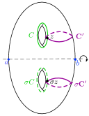
Consider the -surface which can be depicted as a torus with a reflection action as shown in Figure 12. The fixed set is shown in blue. By Theorem 5.9, the cohomology of is
as shown on the grid.
Notice , , , and , . All of these fundamental classes forget to nonzero singular classes, so they must be nonzero. Now in , we have four nonzero elements , , , and . Let’s determine the dependence relations between these classes.
The classes , , and forget to nonzero classes and so cannot equal . Since and are in different components of the fixed set, we can conclude from Corollary 4.5 that they restrict to different classes under the inclusion of the fixed set. Thus . If we forget to singular cohomology then , so by the forgetful long exact sequence, it must be that . We conclude forms a basis for .
Using Theorem 4.10, we have the following multiplicative relations
Let and . We have shown as an -algebra
Example 4.15.
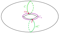
Consider the -surface whose underlying space is the projective plane. To describe the action, recall we can form by identifying antipodal points on the boundary of the disk. The space will inherit the action from the rotation action on the disk, as depicted in Figure 13. The fixed set is again shown in blue. The cohomology of this space is
Let’s consider the submanifold and its normal bundle . The circle is fixed, and for every , the fiber is given by . Thus we have a class . The submanifold has two fixed points , , and while . Thus we also have a class and similarly a class . It is clear . By considering neighborhoods, we also see while .
We have the following multiplicative relations from Theorem 4.10:
Under the inclusion of fixed points , by Corollary 4.5. We show .
Note and both forget to the same nonequivariant nonzero class, so in particular, and . Also since while , we see that . Thus it must be that , and this also shows .
Taking , , we can now state the cohomology of as an -algebra:
Example 4.16 (Fundamental class of conjugate points).
Let be a closed, connected, -dimensional -manifold with a non-fixed point . Consider the set of conjugate points and note this is isomorphic to the free orbit . We show if is free, then for all . If is nonfree, let be a fixed point whose fundamental class generates a free summand in bidegree . We show only for , and explicitly, .
If is free, then the quotient map is a map of smooth manifolds. By Theorem 4.9, and this class is nonzero as described in the proof of Lemma 6.4.
For the nonfree case, we use the long exact sequence for the pair to determine when the class is nonzero. Observe the space is a punctured -manifold, so for . Using the forgetful long exact sequence, we see that
must be an isomorphism whenever and surjective when . If is nonfree, then is also nonfree. Considering the structure theorem and the properties of the action, it must be that no summands in are generated in topological dimension for and all antipodal summands must be concentrated in topological dimension less than . Thus there is a sufficiently small such that whenever .
Fix such that and . Consider the long exact sequence below:
The left group is , and since the second map is surjective, there must be at most one nonzero element in . One such element is , and so the only option is . Now if this holds for some , then it must hold for all by the action of . Lastly for ,
Example 4.17.
Consider the free torus whose action is orientation reversing; this space was denoted earlier in the paper. For notational simplicity, let . An illustration of the space and its cohomology are shown in Figure 14.
There are four families of cohomology classes of interest: , , , and . Observe the classes and forget to nonzero classes in singular cohomology, so and are nonzero for all . Using the long exact sequence for the pair , one can check for all . Now so it must be that is in the image of , and the only possibility is that . By perturbing we can find a submanifold such that and the transverse intersection is empty.
From Theorem 4.10 we have that for all , . This also follows from the module structure and the above fact that , but it is nice to be able to recover the relation using fundamental classes.
The action of on the cohomology of is invertible, and it is easier to describe the cohomology as a -algebra. Note this also encodes the -algebra structure. As a -algebra we have recovered the following isomorphism where :
Example 4.18.
We do one more example that has both nonfree and free fundamental classes. Consider which can be depicted as a genus two torus with a rotation action, as shown below. The cohomology of this space is given by
which is shown in the grid below.
![[Uncaptioned image]](/html/1907.07284/assets/x4.png)
Let’s consider the nonfree fundamental classes , , and the free fundamental classes, and . Note and forget to different nonzero classes, so both are nonzero, and they are not equal. These two families of classes therefore give rise to the two summands appearing. One can also check and using arguments as in the previous examples.
5. Background on -surfaces
In [D2] all -surfaces were classified up to equivariant isomorphism, and furthermore, a language was developed for describing the -structure on a given equivariant surface. We review some of this language and the necessary parts of the classification. We then review the Bredon cohomology of all nonfree -surfaces in -coefficients which was computed in [Ha]. We begin with a few constructions.
Definition 5.1.
Let be a nontrivial -surface and be a nonequivariant surface. We can form the equivariant connected sum of and as follows. Let denote the space obtained by removing a small disk from . Let be a disk in that is disjoint from its conjugate disk and let denote the space obtained by removing both of these disks. Choose an isomorphism . Then the equivariant connected sum is given by
where and for . We denote this space by .
Remark 5.2.
There are two important examples of equivariant connected sums that warrant their own notation. These occur when is one of or , the two nonfree, nontrivial equivariant spheres. We refer to such spaces as doubling spaces, and denote the space by Doub or Doub, respectively. The phrase “doubling” is used to acknowledge that nonequivariantly is homeomorphic to .
The next two constructions involve removing conjugate disks in order to attach an equivariant handle. There are two types of handles that can be attached. The first handle is given by , where is the unit disk in ; we will refer to such a handle as an “antitube”. The second type of handle is given by ; we refer to this handle as an “antitube”. We give the precise definitions below.
Definition 5.3.
Let be a nontrivial -surface. Form a new space denoted as follows. Let be a disk contained in that is disjoint from its conjugate disk . Remove both disks from and then attach an antitube. Whenever we construct such a space, we say we have done surgery.
We can similarly define surgery by instead attaching an antitube.
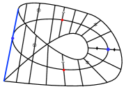
The last type of surgery we recall involves removing a disk isomorphic to the unit disk in and sewing in an equivariant Möbius band. This equivariant Möbius band can be formed as follows. Begin with the nonequivariant Möbius bundle over and then define an action on the fibers by reflection. In other words, each fiber should be isomorphic to (in particular, the zero section is fixed). If we now take the closed unit disk bundle, note the boundary is a copy of , as is the boundary of the removed . An illustration of this Möbius bundle is shown below. Conjugate points are indicated by matching symbols, while the fixed set is shown in blue.
![[Uncaptioned image]](/html/1907.07284/assets/x5.png)
Definition 5.4.
Let be a nontrivial -surface that contains an isolated fixed point . Then there exists an open disk such that . Remove and note . Now sew in a copy of the Möbius band described above. We denote this new space by and refer to this surgery as surgery. (Note “FM” is an abbreviation for “fixed point to Möbius band”.)
5.5. Invariants
When discussing -surfaces, we will often need to refer to certain invariants. The notation for these invariants is given below.
Notation 5.6.
Let be a -surface. Then
-
•
denotes the number of isolated fixed points;
-
•
denotes the number of fixed circles; and
-
•
denotes the dimension of and will be referred to as the -genus of .
When there is no ambiguity about which space is in discussion, we will just write , , and for the respective values.
The complete list of nonfree, nontrivial -surfaces is given in [D2], but we only need the following takeaway for our discussion of fundamental classes.
Theorem 5.7.
Let be a nonfree, nontrivial -surface. If is not isomorphic to a doubling space or to an equivariant sphere, then can be obtained by doing , , or surgery to an equivariant space of lower -genus.
5.8. Bredon cohomology of nonfree -surfaces
We now state the Bredon cohomology of nonfree -surfaces in constant -coefficients which was computed in [Ha, Theorem 6.6]. Note the answer depends only on the -genus and the fixed set.
Theorem 5.9.
Let be a nontrivial, nonfree -surface. There are two cases for the -graded Bredon cohomology of in -coefficients.
-
(i)
Suppose . Then
-
(ii)
Suppose . Then
6. Fundamental classes for -surfaces
It is straightforward to check the singular cohomology in -coefficients of any surface is generated by fundamental classes. In the previous examples, we saw the analogous statement held for the Bredon cohomology of a handful of -surfaces. In this section, we show, in fact, the Bredon cohomology of any -surface is generated by fundamental classes.
Notation 6.1.
As before, the coefficients are understood to be in this section.
We begin by defining the precise property we will be proving.
Definition 6.2.
Let be a -manifold. Suppose there exist a (possibly empty) collection of nonfree equivariant submanifolds and a (possibly empty) collection of free equivariant submanifolds such that the corresponding fundamental classes generate as an -module, i.e.
Then we say is generated by fundamental classes.
Our goal is to show if is any -surface, then is generated by fundamental classes. We begin with free surfaces, spheres, and doubling spaces, and then consider surfaces obtained by doing surgery to such spaces and apply Theorem 5.7.
Warning 6.3.
One might hope the submanifolds can always be chosen to be fixed. This has been the case in our examples thus far, but it is not true in general. For example, consider the torus with the rotation action that has four fixed points (this can also be described as ). By Theorem 5.9 the cohomology of this space is
We claim for any free submanifold , and thus no free submanifold can generate a free summand. To see this, recall is defined as the image of the Thom class of the normal bundle, and the Thom class of a bundle over a free space has -torsion by Theorem 3.17 and Lemma 2.14. On the other hand, the fixed set has codimension , and thus no fixed submanifold can generate the free summands in topological degree . In this case, we need classes that are neither free nor fixed in order to generate the cohomology.
Lemma 6.4.
Suppose is a free -surface. Then is generated by fundamental classes.
Proof.
Since is free, the quotient map is a smooth map of surfaces. Now is generated by fundamental classes of submanifolds, and let denote these submanifolds of . By Theorem 4.9, and we claim the classes for generate the cohomology of . Indeed, by Remark 3.11,
and so the Bredon cohomology of is determined by the singular cohomology of . This completes the proof. ∎
Lemma 6.5.
Suppose is a -sphere. Then is generated by fundamental classes.
Proof.
There are exactly four -spheres up to equivariant isomorphism: , , , and . Note was handled in the above theorem. When is , , or , we need only take the classes and where is some fixed point. These classes will generate . ∎
Lemma 6.6.
Suppose is a doubling space. Then is generated by fundamental classes.
Proof.
There are two cases, either or . The proof for both cases is very similar, so we only provide a proof for the former.
Using Theorem 5.9, the cohomology of is given by
The class will generate the -summand appearing in bidegree , while where is any fixed point is a generator for the -summand appearing in bidegree . Thus we must find one-dimensional submanifolds whose classes will generate the -summands appearing in topological degree one.
Let and be one-dimensional submanifolds of that generate . Note we can choose these submanifolds so that they do not intersect the neighborhood removed from to form . In we will have submanifolds of the form for each . The classes form a basis for , so the classes are linearly independent in . From the forgetful map, these classes must be linearly independent in , and hence they must generate the -summands in topological degree one. This completes the proof. ∎
Our next goal is to show this property holds for all nonfree surfaces. To do so, we make use of Theorem 5.7, which states if is a nontrivial -surface that is not free, not isomorphic to a sphere, and not isomorphic to a doubling space, then up to equivariant isomorphism, can be constructed by doing , , or surgery to a -surface of lower -genus. We first prove a lemma that will be helpful in what follows.
Lemma 6.7.
Let be a nonfree -surface. Suppose is a one-dimensional submanifold such that and . Let be a fixed point. Then where is the inclusion map.
Proof.
Consider the map . Note consists of two isolated points; let and denote these points. By Corollary 4.5, . The lemma then follows by noting can be factored . ∎
We now investigate how doing surgery introduces new fundamental classes.
Lemma 6.8.
Let be a closed -surface such that is generated by fundamental classes. If , then is also generated by fundamental classes.
Proof.
The surface contains a fixed circle, so by Theorem 5.9
where the remaining modules appearing in the decomposition depend on . As usual, the class will generate the free summand appearing in bidegree while if is any point contained in a fixed circle, the class will generate a free summand in bidegree . We just need to find various one-dimensional submanifolds of that generate the remainder of the cohomology. The procedure to find such submanifolds will depend on the isomorphism type of .
Suppose are nonfree one-dimensional equivariant submanifolds of and are free one-dimensional submanifolds of whose fundamental classes together with and generate . Let be equivariant tubular neighborhoods of , respectively. In order to form , we must remove disjoint conjugate disks , from , and we may assume without loss of generality that these disks and the tubular neighborhoods are chosen in a way such that and are empty for all .
Let be the space obtained by removing from . We would like to relate the cohomology of to the cohomology of , and we will use the cohomology of the space as a stepping stone from to .
Observe and can be realized as the homotopy pushouts of the following diagrams, respectively:
Using the diagram on the left, for each we have a long exact sequence:
The map is an isomorphism because on the level of spaces
is the identity, so is an injective map from to . Thus the leftmost map is surjective, and the rightmost map is injective by exactness. Though so the map is injective. The inclusion induces a map ; this map is often not injective, but for each submanifold from our list, we have the following commutative diagram:
Note the top horizontal maps are isomorphisms due to excision: all three of these groups are isomorphic to where is the chosen tubular neighborhood of (note this is why we chose the disks and neighborhoods to be disjoint). The bottom left horizontal map is injective from the above discussion.
In particular, this commutative diagram holds for and . Hence, the image of each of the classes and in under the right horizontal map is equal to the image of the respective class or in under the left horizontal map. The injectivity of the left map shows the fundamental classes inherit no new relations in the cohomology of that were not present in the cohomology of . Intuitively, this is unsurprising: attaching a handle should not introduce dependence relations, and the above formalizes this intuition.
There are three cases for how the cohomology of differs from the cohomology of . First, suppose already contains a fixed oval. Then by Theorem 5.9
| (6.8.1) | ||||
while
Since , we have the following relations
that show
| (6.8.2) |
Recall the classes and generate free summands in topological degrees zero and two, respectively, while the classes generate any summands appearing in topological dimension one coming from by the discussion above. Thus it suffices to find two new fundamental classes in .
There is an obvious choice for one of the submanifolds, namely the fixed circle contained in the attached handle. Let be this circle and note . For the other submanifold, let be a fixed point, and choose a point contained in another fixed circle. It follows from [D2, Corollary A.2] that we can construct a path from to such that
and such that and intersect at the single point . Let be a tubular neighborhood of . Over each fixed point the normal fiber is a fixed interval, so . The two classes are in the correct bidegrees; we next show they are linearly independent from the classes coming from .
We begin with . By construction and intersect at a single fixed point, so
On the other hand, does not intersect any of the other submanifolds , and so for any -linear combination of these fundamental classes
Hence, it must be that is not in the -span of these classes. By the isomorphism in 6.8.1, the fact that is generated by fundamental classes, and consideration of degrees, it must be that
We have already remarked that
By the isomorphism in 6.8.2,
We just proved is not in the -span of the classes , , so by dimensions it must now follow that
Thus any generator of the new summand is a linear combination of fundamental classes.
Returning to , we can apply Lemma 6.7 to see is nonzero. Since does not intersect any of the submanifolds , . For degree reasons, is also zero, and thus any -combination of these classes must be in the kernel of . We conclude is not in the -span of any of these classes. Again using our isomorphisms and degree arguments we can say
We conclude any generator of the new summand is in this span. Thus
as desired. This completes the proof in the case that contains a fixed oval.
Next suppose the fixed set of contains only isolated fixed points. Then by Theorem 5.9
while
We have the relations
Hence the number of and summands match, and we just need to find two new classes that generate the two additional -summands.
As in the previous case, we need to find two new fundamental classes. Again let be the attached (and now only) fixed oval, noting . Let be a path from a fixed point to an isolated fixed point , choosing the path such that
and such that and only intersect at a single point. Let be a tubular neighborhood of the circle , and note that the fiber over is isomorphic to , while the fiber over is isomorphic to , so it must be that .
We can do the same tricks as before to conclude and generate the rest of the cohomology of . Namely, their nontrivial product shows is not an -combination of our current classes. To see is not in the span of the classes given by , choose another point on the fixed oval and use the map . This will complete the proof in this case.
Lastly, suppose is a free -surface. Then by the computations in [Ha], ignoring the action of ,
while by Theorem 5.9
We now have the relations
The number of summands generated in topological dimension one is the same in as in . Thus, by adding and to our list of classes , we will have found a collection of fundamental classes that generate the cohomology of . ∎
Lemma 6.9.
Let be a nontrivial -surface such that is generated by fundamental classes. If , then is also generated by fundamental classes.
Proof.
The proof is similar to that of the previous lemma, so we just provide an outline. Instead of having a fixed circle in the attached handle, we have a circle . The fundamental class for is in bidegree . In the case where has an isolated fixed point, the other class will be given by a circle where is a path from a fixed point on to this other isolated fixed point; this will give another class in bidegree . In the case where only has fixed ovals, the other class will given by a circle where is a path from a fixed point on to a point on a fixed oval. Lastly, in the case where is free, no other classes besides and will be needed. ∎
We are now ready to prove the main theorem of this section.
Theorem 6.10.
Let be a -surface. Then is generated by fundamental classes of equivariant submanifolds.
Proof.
If is trivial, then by Lemma 2.9
Since is generated by fundamental classes, it immediately follows that is generated by fundamental classes.
Assume is nontrivial. We proceed by induction on the -genus of . If the -genus is zero, then we are done by Lemma 6.5. For the inductive hypothesis, let and assume the statement holds for all surfaces of -genus less than .
Let be a surface of -genus . If is a free -surface or a doubling space, then we are done by Lemmas 6.4 and 6.6. Thus suppose is nonfree and not a doubling space. By Theorem 5.7, there are three cases for : the surface is isomorphic to a space given by doing , , or surgery to a surface of lower -genus.
Combining the first and second cases, suppose where . Note , so we can apply the inductive hypothesis to conclude is generated by fundamental classes. We are then done after applying either Lemma 6.8 or Lemma 6.9.
The remaining case is . Let denote a closed neighborhood of the attached Möbius band and observe . Thus in this case we have a map that appears in the cofiber sequence
Note and so it follows from the associated long exact sequence that the map is injective if . Since , the inductive hypothesis implies is generated by fundamental classes. Let be the nonfree and be the free the one-dimensional submanifolds of whose fundamental classes along with and generate . We can choose these submanifolds so that and are submanifolds of . By Theorem 4.9, and similarly . The injectivity of implies these classes inherit no new relations in . Similar to the proof of Lemma 6.9, our goal is to find new submanifolds to generate the remainder of . There are two subcases based on the fixed set of .
First suppose contains a fixed circle. Then by Theorem 5.9,
so we just need to find a single one-dimensional submanifold. Let denote the circle in the attached Möbius band. Then gives a class in bidegree . As in Lemma 6.9, construct a circle from a path that travels from a point on to a point on another fixed circle. Then . From the intersection product, while and for all , , and . Thus must be linearly independent from the classes already in . We conclude the classes , , , , and where is any point on a fixed circle will generate .
Next suppose does not have any fixed circles. The fixed set of must contain at least one fixed point in order to do surgery. By running the long exact sequence associated to the cofiber sequence (or by Theorem 5.9), we see has the same number and type of summands generated in topological degree one as except it has an additional summand of the form . Let be a fixed point on . In this case, the classes , , , , and will generate .
We have exhausted all cases, and we conclude is generated by fundamental classes for all -surfaces. ∎
Appendix A An algebraic property of -modules
In this appendix, we state and prove a theorem about maps between nice -modules that are isomorphisms in a certain range. This theorem will imply property (vi) of Theorem 3.16.
Notation and terminology
We say an -module is “nice” if it is a direct sum of finitely many copies of shifted free modules and shifted copies of for various values of , and furthermore, if all shifts are given by actual representations, i.e. the shifts are given by where . We will refer to the -summands as “antipodal summands”. Given an antipodal summand of the form , we can associate the tuple ; note an antipodal summand with tuple begins in topological dimension and ends in topological dimension . Given an -module and an element we will write for the weight of . When considering a single bidegree, we will write for the elements of in bidegree .
In the proof, we will consider certain quotients, submodules, and localizations of nice -modules in order to detect the properties of free versus antipodal summands. For an -module let . If is a nice module, note consists of the antipodal summands and the bottom cones of free summands. We can then consider the quotient which is isomorphic to a direct sum of top cones, one for each free summand in . We will denote such quotients by . If we further quotient to form , we obtain a module isomorphic to a direct sum of shifts of the module , one for each free summand. We can also consider the localization which is isomorphic to the antipodal summands of .
We begin by proving a lemma about -modules which will be useful when considering the quotient .
Lemma A.1.
Consider the graded polynomial ring where . Let be a finitely generated, free -module with -basis . Suppose is another finitely generated, free -module, and is a degree map such that is an isomorphism whenever for some integer . Then there exists an -basis for such that .
Proof.
There exist integers such that is larger than and constant for all . The elements form a linearly independent set in and thus the images form a linearly independent set in . This implies there are at least free summands in . We can similarly use in the range it exists to show there can be at most free summands in . We conclude has an -basis consisting of elements.
We proceed by induction on to show there is a basis for such that . This is clear if the bases consist of exactly one element since otherwise would be zero. For the inductive hypothesis, suppose we can find such a basis whenever we have a map that is an isomorphism in sufficiently high degrees between finitely generated, free -modules of rank . Choose some -basis for and suppose where . Let be a basis element of maximal degree such that the coefficient is nonzero. Reorder the set so that this element is now . We can factor out powers of to obtain
Let and note the set is still an -basis for . Furthermore, we obtain a map
that is still an isomorphism in the desired range. By the inductive hypothesis, there exists an -basis for the quotient such that . Let be a lift of to . Then will be a basis for such that . ∎
Theorem A.2.
Let and be two nice -modules such that has free summands generated in bidegrees and antipodal summands with tuples . Suppose is an -degree -module map such that is an isomorphism whenever . Then has exactly free summands generated in bidegrees such that and exactly antipodal summands with tuples .
Proof.
One readily checks the restrictions and are isomorphisms in the given range. The map then descends to a map
that is still an isomorphism when . The quotients and are isomorphic to a direct sum of shifts of the module , one for each free summand in and , respectively. Explicitly
Fix a topological dimension and consider and . These are both finitely generated, free -modules and the map
is an isomorphism whenever . By Lemma A.1, there are respective bases and for and such that . Lifts of the elements and to and will generate the free summands in bidegrees and in and , respectively. This proves the statement about the free summands.
We next consider the antipodal summands. Consider the localization . Let and note is a finitely generated -module. By the decomposition of into summands as an -module, we can say explicitly
Similarly is isomorphic to a direct sum of shifts of , one for each antipodal summand of .
Note restricts to a map which then localizes to give a map of finitely generated -modules. Since was an isomorphism in bidegrees such that , the map is guaranteed to be an isomorphism in these bidegrees. Though, now that is invertible, we see that is an isomorphism in all bidegrees. We conclude and must have exactly antipodal summands with tuples . ∎
References
- [AM] S. Araki, M. Murayama, -cohomology theories, Japan J. Math. (N.S.) 4 (1978), no. 2, 363-416.
- [CHT] S. R. Costenoble, T. Hudson, S. Tilson, The -equivariant cohomology of complex projective spaces. Preprint (2018). arXiv:1811.07355
- [CW] S. R. Costenoble, S. Waner, Equivariant Poincaré duality, Michigan Math. J. 39 (1992), no. 2, 325–351.
- [D1] D. Dugger, An Atiyah-Hirzebruch spectral sequence for -theory, -Theory 35 (2005), no. 3–4, 213–256.
- [D2] D. Dugger, Involutions on Surfaces, Journal of Homotopy and Related Structures (2019).
- [Ha] C. Hazel, The -graded cohomology of -Surfaces in -coefficients. Math. Z. (2020).
- [HHR] Hill, M. A.; Hopkins, M. J.; Ravenel, D. C. On the nonexistence of elements of Kervaire invariant one. Ann. of Math. (2) 184 (2016), no. 1, 1–262.
- [Ho] E. Hogle, -graded cohomology of equivariant Grassmannian manifolds,. Preprint (2018). arXiv:1806.01537
- [K1] W. C. Kronholm, A freeness theorem for -graded cohomology, Topology Appl. 157 (2010), no. 5, 902–915.
- [K2] W. C. Kronholm, On the equivariant cohomology of rotation groups and Stiefel manifolds. Preprint (2011). arXiv:1107.5865
- [L] L. G. Lewis, The -graded equivariant ordinary cohomology of complex projective spaces with linear actions, appearing in Algebraic topology and transformation groups, ed. tom Dieck, Lecture Notes in Math., vol. 1361, Springer, 1988.
- [LFdS] P.F. dos Santos and P. Lima-Filho, Bigraded incariants for real curves, Algebr. Geom. Topol. 14 (2014), no. 5, 2809–2852.
- [M1] C. May. A structure theorem for -graded Bredon cohomology. Algebr. Geom. Topol. 20 (2020), no. 4, 1691–1728.
- [M2] J. P. May, Equivariant homotopy and cohomology theory, published for the Conference Board of the Mathematical Sciences, Washington, DC, with contributions by M. Cole, G. Comezaña, S. Costenoble, A.D. Elmendorf, J.P.C. Greenlees, L.G. Lewis Jr., R.J. Piacenza, G. Triantafillou, S. Waner, CBMS Reg. Conf. Ser. Math 91 (1996).
- [Se] G. Segal, Equivariant -Theory, Publications Mathématiques de l’IHÉS 34 (1968), 129–151.
- [Sh] M.E. Shulman, Equivariant local coefficients and the RO(G)-graded cohomology of classifying spaces, Doctoral dissertation (2010), University of Chicago. arXiv:1405.1770
- [T] R. Thom, Quelques propriétés globales des variétés différentiables, Commment. Math. Helv. 28 (1954), 17–86.