Cooperative UAVs Gas Monitoring using Distributed Consensus

Abstract

This paper addresses the problem of target detection and localisation in a limited area using multiple coordinated agents. The swarm of Unmanned Aerial Vehicles (UAVs) determines the position of the dispersion of stack effluents to a gas plume in a certain production area as fast as possible, that makes the problem challenging to model and solve, because of the time variability of the target. Three different exploration algorithms are designed and compared. Besides the exploration strategies, the paper reports a solution for quick convergence towards the actual stack position once detected by one member of the team. Both the navigation and localisation algorithms are fully distributed and based on the consensus theory. Simulations on realistic case studies are reported.

I Introduction and related works

Unmanned Aerial Vehicles (UAVs), RPA (Remotely Pilot Aircraft) are nowadays used for a large variety of applications, such as structural monitoring [1], emergency scenarios like search and rescue [2], target tracking and encircling [3], reaching close to commercial solutions in some cases [4], or environmental monitoring [5, 6].

The goal of this work is to localise the emission source of the gas dispersion as fast as possible as proposed in [7], using multiple autonomous UAVs, and specifically, quadrotors [8], to speed up the task of seek-and-find. Our solution consists of two steps: the first concerns the exploration strategies towards the gas source detection, the second focuses on the distributed localisation once the source has been detected.

The use of coordinated multiple agents is of course not novel in the literature. In particular, it has been shown that the information exchange between the agents of a team reduces to time to accomplish a mission, which can be theoretically demonstrated, for example applying the consensus theory [9]. In this framework, UAV formation control using a completely distributed approach among the controlled robots is a field already investigated in the literature [10].

Once the stack has been detected, the UAVs have to estimate its position. The literature for target tracking is quite rich [11, 12], especially when the target is not governed by a white noise but, instead, has a strong correlation between the executed manoeuvres [13]. Assuming that the target is not moving but it is standing in a fixed unknown location has also been presented in the literature, for example by [14, 15] using distributed consensus-based known algorithms.

Gas source localisation is considered in [16] using the “Grey Wolf Optimiser”, a recently developed algorithm inspired by grey wolves (Canis lupus). It consists of three-stage procedure: tracking the prey, encircling the prey, and attacking the prey. This algorithm works with a minimum of $4$ agents and, increasing the agent number beyond seven, caused the reduction in success rate (percentage of success in gas source localisation, $72\%$ with $7$ agents) and increase the time to completion, due to increased frequency of irrecoverable collisions between robots.

In this paper, three exploration algorithms for swarms of UAVs conceived for gas source localisation are proposed and are based on i) coordinated scanning, ii) Random walk and iii) Brownian motion. All share the same method: as long as one agent senses the gas with a concentration greater than a certain threshold, it becomes the master of the group and the source localisation phase starts. In this latter phase, the agents are controlled with a distributed algorithm that dynamically allocates the master role and localises the source. The algorithms presented in this paper converge on the maximum concentration point, which is a property shared with the Particle Swarm Operation [17] and the Ant Colony Optimisation [18] approaches. Nonetheless, there are some differences with respect to the discussed literature, the most relevant being the approach adopted to find the source. In fact, in the Grey Wolf Optimiser, agents start in a zone where the concentration of the gas is above a minimum sensing threshold, and this data is necessary to reach the source; in our case, instead, UAVs can start in any part of the environment. Moreover, we can statistically prove through extensive simulations that our algorithms can operate also with 2 drones instead of a minimum of 4 and that the rate of success under the presented assumptions is 100%. Finally, for the estimation problem as well as for the exploration, we have considered a limited sensing range for the UAVs.

The paper is organised as follows. Section II introduces the adopted models and presents the problem at hand. Then, in Section III and in Section IV the algorithms used for the area exploration and the source localisation are defined. Section V presents extensive simulations analysing all the relevant features of the algorithms and their comparison. Finally, Section VI draws the conclusions and discusses possible future developments.

II Problem Formulation and Adopted Models

The problem we are aiming at is the detection and localisation of a certain phenomenon (pollutant leak) taking place in an unknown location (stack) inside the environment of interest. The phenomenon is supposed to be measurable by a sensor rigidly fixed on the robot chassis and capturing the intensity of the pollutant concentration. More precisely, if $\langle G\rangle=\{O_{g},\,X_{g},\,Y_{g},\,Z_{g}\}$ is a fixed ground reference frame, where $O_{g}$ identifies the origin of $\langle G\rangle$, the drone can be modelled as an unconstrained rigid body having $6$ degrees of freedom. The position of its centre of mass in $\langle G\rangle$ (which will be considered as the reference point of the drone) is given by $\xi=[x,y,z]^{T}$. Considering that the UAV dynamics is given by a quadrotor and recalling that quadrotors are controlled by differentially driving the four motors, we will make use of the results in [19] to decoupling the attitude and position control. In practice, given a desired position $\xi^{*}$ to be reached, it is possible to generate a vertical thrust $u_{1}$ and a torque vector $u_{2}$ around its centre of mass to steer the UAV towards $\xi^{*}$. To this end, a suitable trajectory planner generating smooth trajectories connecting the starting and ending position of the quadrotor is utilised (this component is not described in this paper, but it is quite customary in the literature). The UAV model thus considered is approximated, since:

• The model does not take into account actuation saturations, while in reality this is a major issue for this robotic systems. Therefore, we assume the linear velocity limited to $3$ m/s;

• We have supposed to be capable of measuring the whole state. In practice a nonlinear observer is adopted [19];

• We have not modelled several aerodynamic effects [19]. For instance, if the robot is flying at high speed, they become no more negligible.

We consider these approximations acceptable in this work since we are more interested in the distributed coordination of the UAVs formation, making them a team of autonomous agents, instead of giving a too much detailed analysis of the single agent dynamic. As a result, the individual UAV can be considered to be controlled by generating a set of desired configurations to be reached. In particular, we will assume that the $i$–th agent dynamic, with $i=1,\dots,n$ is given as a first order integrator, i.e.

$$\dot{\xi}_{i}(t)=u_{i}(t),$$ (1)

where $u_{i}\in\mathbb{R}^{3}$ are the three independent control inputs, hence $\xi_{i}=[x_{i},y_{i},z_{i}]^{T}$. The UAVs are supposed to be equipped with GPS sensors to determine the UAV location with negligible uncertainty. For the agents orientation, a magnetic compass is considered. As a consequence, we will refer to $\xi_{i}$ as the actual position of the $i$-th quadrotor in the reference frame $\langle G\rangle$.

II-A Gaussian Plume

Gaussian Plume [20] is a well-known method used to simulate the behaviour of pollutant mixture released in atmosphere by a source in position $p_{s}=[0,0,H_{s}]^{T}$ expressed in $\langle G\rangle$, under the effect of the wind (see Figure 1).

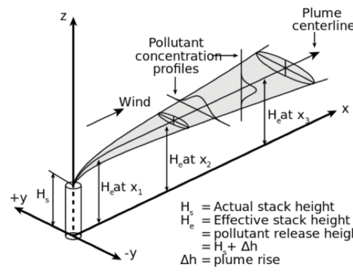
Figure 1: Visualisation of a buoyant Gaussian air pollutant dispersion plume [20].

With the wind blowing, e.g., in the $X_{g}$ direction with speed $w$ measured in meters per second, the plume spreads as it moves along $X_{g}$. In particular, the local concentration $C(x,y,z)$ at a given point $(x,y,z)$ forms distributions which have shapes that resembles Gaussian distributions along the $Y_{g}$ and $Z_{g}$ axes as described in Figure 1. The two modelling distributions are given respectively by $p_{\star}(\star)=\frac{1}{\sqrt{2\pi}\sigma_{\star}(x)}e^{-\frac{\star^{2}}{2\sigma_{\star}^{2}(x)}}$, with $\star=y,z$ and where the standard deviations $\sigma_{y}(x)$ and $\sigma_{z}(x)$ of these Gaussian probability density functions (pdfs) are a function of $x$, i.e. the spread increases with the distance $x$ from the source. At atmospheric stability conditions and using the so called Pasquill-Gifford Curves [21], we have $\sigma_{y}(x)=cx^{d}$ and $\sigma_{z}(x)=ax^{b}$, whose parameters can be found in the well-known Pasquill Gifford stability tables [21].

Assuming as customary the two random variables modelling the plume spread independent, we have that the joint pdf $p_{y,z}(y,z)=p_{y}(y)p_{z}(z)$ and hence the concentration is

$$C(x,y,z,H_{s})= \frac{Q}{w}\frac{1}{2\pi\sigma_{y}(x)\sigma_{z}(x)}e^{-\frac{y^{2}}{2\sigma_{y}^{2}(x)}}\cdot$$ (2)

$$\cdot\left[e^{-\frac{(z-H_{s})^{2}}{2\sigma_{z}^{2}(x)}}+e^{-\frac{(z+H_{s})^{2}}{2\sigma_{z}^{2}(x)}}\right],$$

which accounts for the ground effect and where $Q$ is the dispersion mass and $w$ is the wind speed.

For the concentration sensor, the MiniPID 2 PID sensor, by Ion Science, is supposed to be available. This type of device is a PID (photoionisation detector) sensor, able to sense volatile organic compounds in challenging environments. Assuming that a gas source is positioned in $p_{s}=[x_{s},y_{s},H_{s}]^{T}$ and that the $i$–th robot is located in position $\xi_{i}$, the gas concentration measured in the sensor position (here assumed co-located with the UAV centre of mass without loss of generality) is a modified version of (2), i.e.

$$C_{i}(\xi_{i},p_{s})= \frac{Q}{w}\frac{1}{2\pi\sigma_{y}(x_{i}-x_{s})\sigma_{z}(x_{i}-x_{s})}e^{-\frac{(y_{i}-y_{s})^{2}}{2\sigma_{y}^{2}(x_{i}-x_{s})}}\cdot$$ (3)

$$\cdot\left[e^{-\frac{(z_{i}-H_{s})^{2}}{2\sigma_{z}^{2}(x_{i}-x_{s})}}+e^{-\frac{(z_{i}+H_{s})^{2}}{2\sigma_{z}^{2}(x_{i}-x_{s})}}\right].$$

Considering the limited range of the sensor, we finally have that the measurement results are given by

$$h_{i}(\xi_{i})=\mbox{sat}\left(C_{i}(\xi_{i},p_{s})\right),$$ (4)

where $\operatorname{sat}(\alpha)$ is equal to $\alpha$ if $\alpha<100$, otherwise $\alpha=100$ (maximum sensing range).

II-B Problem Formulation

Consider a set of $n$ UAVs flighting at the same height, i.e. on a generic $X_{g}\times Y_{g}$ plane, and a gas source position $p_{s}=[x_{s},y_{s},H_{s}]^{T}$. Assuming that the $i$–th robot is located in position $\xi_{i}$, the problem is to estimate the plane position $\hat{p}_{s}=[\hat{x}_{s},\hat{y}_{s}]^{T}$ of the source with an error $e_{s}=[x_{s}-\hat{x}_{s},y_{s}-\hat{y}_{s}]^{T}$ such that $\|e_{s}\|\leq\rho_{m}$.

III Exploration Strategy for Stack Detection

The concept of multiple autonomous systems, i.e. computerised systems composed of multiple intelligent agents that can interact with each other through exchanging information, has been proposed for instance in [12]. The use of multiple autonomous systems is usually more efficient than single agent systems from both the task performance and the computational efficiency viewpoints, besides the fact that some problems are difficult or impossible for single agents. Regarding coordination between agents, consensus control approaches have gained a lot of attention for autonomous agents coordination [9]. The main objective is to find a consensus algorithm between the multiple autonomous agents making use of local information and with the aim to control the group using agreements schemes.

Assuming the simple linear dynamic in (1), a quite simple consensus algorithm that let the $n$ agents to converge in a fixed position (rendezvous problem) is the following:

$$\overline{u}_{i}(t)=\sum_{j=1}^{n}l_{ij}(\xi_{i}(t)-\xi_{j}(t)),$$

where $l_{ij}$ is the element in position $(i,j)$ of the Laplacian matrix; if the final positions have to be separated by relative position vectors $\delta_{i}$, then

$$\overline{u}_{i}(t)=\sum_{j=1}^{n}l_{ij}\left[(\xi_{i}(t)-\xi_{j}(t))-(\delta_{i}-\delta_{j})\right],$$ (5)

i.e., the UAVs reaches a final fixed formation. From this simple idea, many different approaches can be applied using the concepts of adjacency and Laplacian matrices [9].

III-A Coordinated Scanning

One simple and effective approach is to use a leader-follower formation: the leader is in charge of moving inside the environment using a controlled reactive behaviour or just following a predefined trajectory (that is the solution here considered), while the followers are adapt to the leader’s motion to preserve the formation. Using [22] and assuming that the $i$–th agent is the leader, it is possible to use

$$u_{i}(t)=\dot{\xi}_{d}(t)-k_{i}(\xi_{i}(t)-\xi_{d}(t)-\delta_{i})+\overline{u}_{i}(t),$$ (6)

where $\overline{u}_{i}(t)$ is reported in (5), $\xi_{d}(t)$ is the desired trajectory, $\dot{\xi}_{d}(t)$ the desired trajectory dynamic and $k_{i}>0$ is a tuning parameter. Similarly, for the $k$-th follower, with $k\neq i$,

$$u_{k}(t)=\frac{1}{\sum_{j=1}^{n}a_{ij}}\left[\sum_{j=1}^{n}a_{ij}\dot{\xi}_{j}(t)+\overline{u}_{i}(t)\right],$$ (7)

where, again, $\overline{u}_{k}(t)$ is in (5) and $a_{ij}$ is the element in position $(i,j)$ of the adjacency matrix. Notice that this algorithm is entirely distributed and the information that the $k$-th agent shares are its position $\xi_{i}(t)$, velocity $\dot{\xi}_{i}(t)$, and its formation vector $\delta_{i}$.

For the coordinated scanning, all the agents can start from an arbitrary position and using (5) converge to a line. In particular, we select as leader the $l=\left\lceil(n/2)\right\rceil$ agent (any other heuristic for the leader choice can be applied), which is in fixed position, i.e. $u_{l}(t)=0$, and has $\delta_{l}=[0,0,0]^{T}$. For any other agent $i\neq l$, we make use of (5) with $\delta_{i}=[0,-(l-i)\Delta_{y},0]^{T}$, where $\Delta_{y}=20$ m is the desired distance along the $Y_{g}$ axis. This way, the UAVs are placed on a line parallel to $Y_{g}$ (see Figure 2).

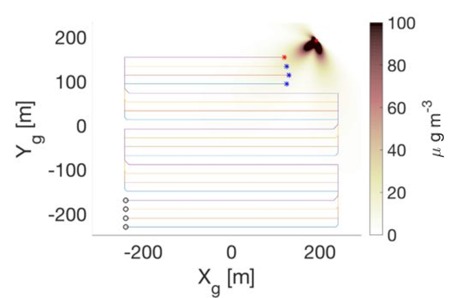
Figure 2: Example of coordinated scanning. UAVs start from an initial configuration (circles) that is a line and scan the whole area until one of the team members (red star) does not detect a sufficiently high gas concentration (stars in the final configuration).

Once this initial configuration is reached, the exploration starts. In the example of Figure 2, the exploration follows lines that are parallel to the $X_{g}$ axis, hence the leader desired velocity in (6) is set to $\dot{\xi}_{d}=[\pm v_{m},0,0]^{T}$ for motions parallel to the $X_{g}$ direction or to $\dot{\xi}_{d}=[0,v_{m},0]^{T}$ when are moving upwards along the $Y_{g}$ direction. In the simulations of Figure 2 the UAV velocities are set to $v_{m}=3$ m/s and a wedge formation is chosen. The decision to switch between the different directions is taken by the leader knowing the dimension of the area to scan, while the motion switches from vertical to horizontal whenever the leader has travelled for a distance of $d=n\Delta_{y}$.

III-B Random Walk

We simulate a random walk for the motion of the UAVs inside the area of interest. In this case, the $i$–th agent moves according to this dynamic

$$\dot{\xi}_{i}(t)=\begin{bmatrix}\cos(\theta_{i}(t))\\ \sin(\theta_{i}(t))\\ 0\end{bmatrix}v_{m},$$

that is computed every $\Delta_{t}$ seconds and in which the orientation $\theta_{i}(t)$ is updated following the update rule $\theta_{i}(t)=\theta_{i}(t-\Delta_{t})+\nu$, being $\nu\sim\mathcal{U}(-\theta_{M},\theta_{M})$ a random variable uniformly distributed and generated by a white stochastic process, where $\theta_{M}$ is a user defined constant. Hence, the name random walk for this exploration strategy. Whenever the $i$-th agent reaches the area of interest border, a new orientation is randomly generated according to $\theta_{i}(t)=\nu\theta_{\mbox{in}}\theta_{r}/\theta_{M}$, where $\theta_{\mbox{in}}$ is the orientation of the angle of the local normal vector of the border and pointing inwards the region, while $\theta_{r}$ is a user defined constant threshold describing the feasible orientations originating from a border location. For this particular strategy, a collision avoidance mechanism is needed (recall that all the UAVs are moving at the same height). In this paper, we adopt a quite straightforward solution: whenever the distance between the $i$–th and the $j$–th agent is less than a given safety threshold $d_{m}$, i.e., $\|\xi_{i}(t)-\xi_{j}(t)\|_{2}\leq d_{m}$, the agents are subjected to a repulsive force along the directions $\theta_{i}(t)=\arctan\left(\frac{y_{i}(t)-y_{j}(t)}{x_{i}(t)-x_{j}(t)}\right)$ and $\theta_{j}(t)=\theta_{i}(t)+\pi$ . A simulation explaining this behaviour is reported in Figure 3-(a), where $\theta_{M}=10^{\circ}$ and $\theta_{r}=75^{\circ}$.

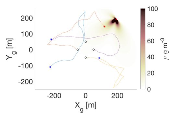
Figure 3: Example of random walk algorithm. UAVs start from an initial configuration (circles) that is a circle centred at the origin and scan the area until one of the team members (red star) does not detect a sufficiently high gas concentration (stars in the final configuration).

The initial configuration (circles) is on a circle centred at the origin and with radius $50$ m.

III-C Brownian Motion

The final exploration strategy is dubbed Brownian motion. According to the basic rules of Brownian motion particles, in this work the random change in direction of the agents is determined by two events: collision avoidance intervention and boundary collision.

IV Localisation of the Stack

Since all the UAVs in the team has the capability of sensing the gas concentration using the sensor described in Section II-A, once any of the team members detects it, it becomes the new leader of the formation (signed with a red star in Figure 2 and Figure 3). This type of information, together with position data, are shared with other agents and the localisation phase starts. The algorithm works as follows:

1. At the beginning, the team is arranged in a circle of radius $r$ with the current leader acting as the fixed circle centre. The positions on the circle are determined by letting the leader, say the $j$–th agent, computing the position vectors $\delta_{i}$, $i\neq j$ using polar coordinates, for all the agents and then applying (7);

2. When the circle formation is reached, the $n-1$ UAVs move along a logarithmic spiral with the $i$-th agent radius $r_{i}=re^{b\beta_{i}}$, where $\beta_{i}$ is the arc spanned by the $i$-th agent around the leader from the initial circle position and the fixed coefficient $b$ is computed in order to have a reduction on the radius between two agents position of $\gamma\rho_{m}$, where $\rho_{m}$ is the maximum allowed error defined in Section II-B. In particular, $b=\frac{n-1}{2\pi}\log\frac{r-\gamma\rho_{m}}{r}$;

3. If the $i$–th agent along the spiral motion detects a gas concentration larger than the actual leader, i.e.

   $$h_{i}(\xi_{i})>h_{j}(\xi_{j}),$$

   then the $i$–th agent becomes the leader and the algorithm starts over from Step 1;

4. The spiral motion for all the agents ends when $r_{i}=\rho_{m}$, i.e. the desired tolerance of Section II-B;

5. At this point, the agents start to move on the circle with radius $\rho_{m}$ for an arc of length $2\pi/(n-1)$;

6. If the $i$–th agent along this arc-circle motion verifies the gas concentration condition $h_{i}(\xi_{i})>h_{j}(\xi_{j})$, the $i$–th agent becomes the leader and the algorithm restarts from Step 5. Otherwise the algorithm ends.

The algorithm thus designed works assuming that the gas concentration is a decreasing function of the distance from the source, which is verified by the Gaussian plume model described in Section II-A.

V Simulation Results

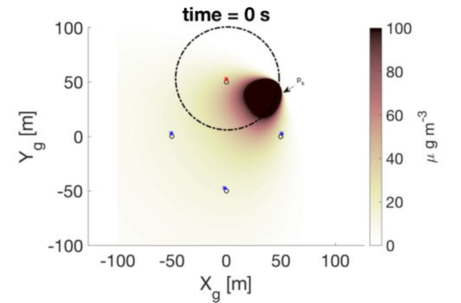
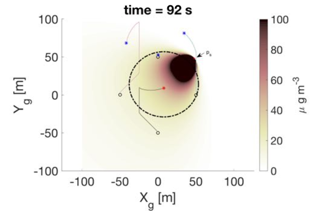
(a)	(b)
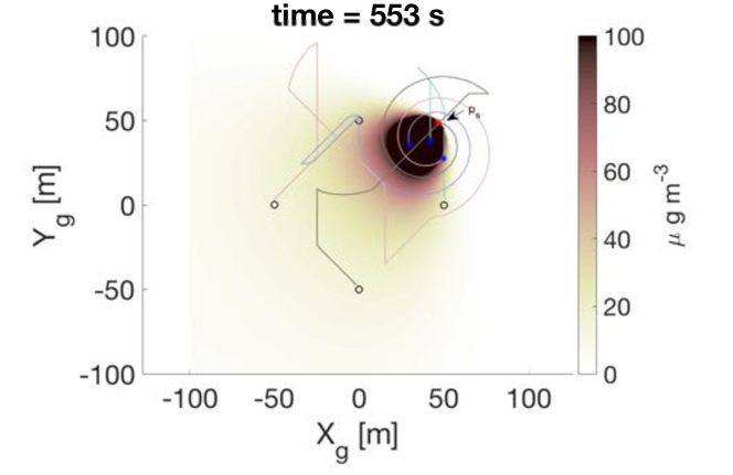
(c)	(d)

Figure 4: Four UAVs trajectories during the localisation phase of the stack in position $p_{s}$. (a) At the beginning, the UAVs are requested to move on a circle (dash-dotted line) around the leader (red star). (b) After 92 seconds, the leader changes (red star), with a new desired circle (dash-dotted line). (c) After $132$ seconds, a new leader reaches the desired circle and immediately becomes the new leader (red star). (d) After moving on logarithmic spirals, a new leader is detected, which is quite close to the source $p_{s}$. The overall trajectories followed by the four UAVs are depicted with solid lines.

In this section, we propose a statistical comparison and analysis of the effectiveness of the designed algorithms. This simulative analysis is strictly necessary since many variables come into play, i.e. the different exploration strategies, the behaviour of the Gaussian plume, the number of UAVs. In all the simulation here presented we assume a maximum UAV velocity of $v_{m}=3$ m/s, a stack height $H_{s}=3$ m (which is equal to the agents flighting height), a stack emission of $5$ g/s and a searching area of about $880\times 880$ m². Statistical data have been collected along $m_{s}=100$ simulations in each considered configuration, $m_{w}=100$ different Gaussian plume conditions as well as a variable number of UAVs, from $2$ to $20$ agents. Depending on the particular simulation set-up, each simulation lasts for a variable number of $m_{t}$ samples, where the sampling time is denoted as $\Delta_{t}=1$ s as in Section III.

V-A Pasquill-Gifford model

First, we present the results of the Pasquill-Gifford model presented in Section II-A. The gas dispersion has been modelled considering different conditions. Inspired by [23], a synthetic dataset has been generated based on experimental observations: a) wind coming from a constant direction; b) wind coming from a completely random direction; c) wind coming from a prevailing random direction. All the simulations have been carried out considering very unstable wind conditions. The concentration of the gas mixture in every point of the area are time averaged along the simulation in order to avoid transient conditions happening at the very beginning of the gas leak emission. Figure 4 depicts the simulation results with colours identifying the concentration and the red dot representing the position of the source.

V-B Exploration Strategies

For the statistical analysis of the three different exploration strategies presented in Section III the minimum detection threshold for each agent is $h_{m}=30$ parts per billion, i.e. conservatively $6$ times the rated sensitivity of the sensor described in Section II-A. Figure 5 depicts the mean average taken to complete the mission, i.e. until $\exists i$ such that $h_{i}(\xi_{i})>h_{m}$ as a function of the number of UAVs.

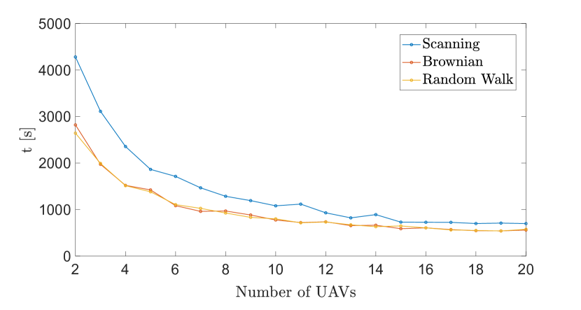
Figure 5: Time to accomplish the mission as a function of the number of UAVs.

Trivially, all the different algorithms behave better increasing the number of drones. Another important aspect that is underlined by the graph is the fact that an algorithm based a deterministic approach has typically worse performance than random exploration approaches, such as Brownian motion and random walk.

V-C Localisation of the Stack

We will now present the results of the source localisation algorithm. The maximum tolerable error is set to $\rho_{m}=5$ m. The radius of the circle arranged at the beginning of the localisation phase is set to $r=50$ m. The ratio governing the contraction of the radius for the logarithmic spirals is set to $\gamma=1/4$. An example of a localisation manoeuvre for $4$ UAVs is reported in Figure 4. At the beginning (Figure 4-(a)), the UAVs are requested to move on a circle (dash-dotted line) around the leader (red star), which is the first sensing a concentration greater than $h_{m}$. After that all the UAVs have reached the circle and started to move along the spiral (after $92$ s, Figure 4-(b)), the leader changes (red star) and a new desired circle (dash-dotted line) is established. The UAVs start moving toward the new circle and, right after $40$ second,s they reached it: a new leader is then immediately determined (red star in Figure 4-(c)). At this point, the UAVs move toward the new circle and start the spiral motions. Then, at time $553$ s, one of the UAVs senses a high level of concentration, and becomes the new leader, denoted with the red star in Figure 4-(d). Even though this new leader is quite close to the source $p_{s}$, the process continues in this way, changing two additional leaders and ending after $721$ s.

To clearly state the performance of this approach, we will start by first saying that the average of the localisation error $\|e_{s}\|$ defined in Section II-B along all the simulations does not vary in a significant way for the three algorithms and it stabilises around $1.6$ m $<\rho_{m}$. Moreover, Figure 6 shows that the condition $\|e_{s}\|<\rho_{m}$ is always verified by design. As a concluding remark, the exploration strategy adopted does not play any role in the final accuracy, while the number of UAVs reduces the exploration time.

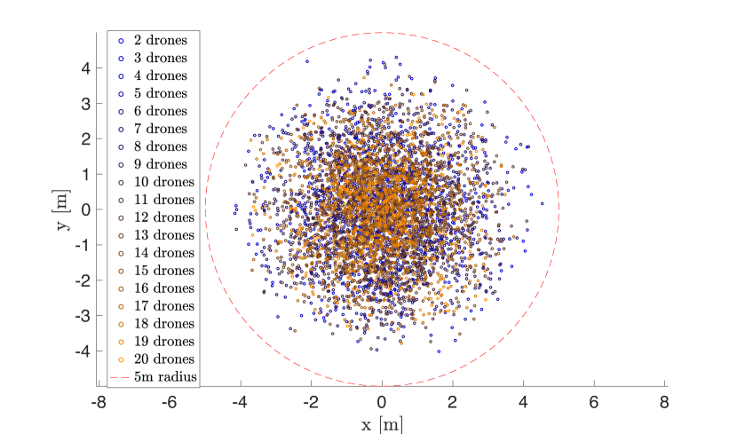
Figure 6: Scattering plot of the error $\|e_{s}\|$.

VI Conclusions

In this paper we have designed and analysed a multi-agent system conceived for the detection of a source of a gas dispersion. Methods based on random motions, such as Brownian motion and random walk here presented, perform averagely better in terms of completion time with respect to deterministic approaches, such as the coordinated scanning here proposed. For the maximum time of mission completion, deterministic approaches offer stringent guarantees, while stochastic approaches can be sometimes excessively high. The final accuracy of the source position is based on a common distributed algorithm designed on purpose. Moreover, we have shown how the number of agents in the team improves the exploration algorithms performance, while it has negligible effects on the localisation accuracy.

Future research directions will be focused on the actual deployment of the algorithms in real scenarios, on the definition of more flexible distributed control approaches as well as on the multiple sources scenarios.

References

- [1] H. Yoon, J. Shin, and B. F. Spencer Jr, “Structural displacement measurement using an unmanned aerial system,” Computer-Aided Civil and Infrastructure Engineering, vol. 33, no. 3, pp. 183–192, 2018.
- [2] G. Seminara and D. Fontanelli, “First Responders Robotic Network for Disaster Management,” in Modelling & Simulation for Autonomous Systems (MESAS), J. Mazal, Ed. Cham: Springer International Publishing, 2018, pp. 350–373.
- [3] F. Morelli, D. Vignotto, and D. Fontanelli, “Modelling of a Group of Social Agents Monitored by UAVs,” in Modelling & Simulation for Autonomous Systems (MESAS), J. Mazal, Ed. Cham: Springer International Publishing, 2018, pp. 40–58.
- [4] Amazon, “Amazon Proposes Drone Highway As It Readies For Flying Package Delivery,” 2015, https://www.forbes.com/sites/ryanmac/2015/07/28/amazon-proposes-drone-highway-as-it-readies-for-flying-package-delivery/#295d90ef2fe8.
- [5] M. Rossi, D. Brunelli, A. Adami, L. Lorenzelli, F. Menna, and F. Remondino, “Gas-drone: Portable gas sensing system on uavs for gas leakage localization,” in IEEE SENSORS 2014 Proceedings, Nov 2014, pp. 1431–1434.
- [6] M. Rossi and D. Brunelli, “Ultra low power mox sensor reading for natural gas wireless monitoring,” IEEE Sensors Journal, vol. 14, no. 10, pp. 3433–3441, Oct 2014.
- [7] V. Gallego, M. Rossi, and D. Brunelli, “Unmanned aerial gas leakage localization and mapping using microdrones,” in 2015 IEEE Sensors Applications Symposium (SAS), April 2015, pp. 1–6.
- [8] H. Huang, G. Hoffmann, S. Waslander, and C. Tomlin, “Aerodynamics and control of autonomous quadrotor helicopters in aggressive maneuvering,” in Proc. of IEEE Intl. Conf. on Robotics and Automation (ICRA), May 2009, pp. 3277–3282.
- [9] W. Ren, R. W. Beard, and E. M. Atkins, “A survey of consensus problems in multi-agent coordination,” in American Control Conference, 2005. Proceedings of the 2005. IEEE, 2005, pp. 1859–1864.
- [10] X. Zhu, Z. Liu, and J. Yang, “Model of collaborative uav swarm toward coordination and control mechanisms study,” Procedia Computer Science, vol. 51, pp. 493–502, 2015.
- [11] X. R. Li and V. P. Jilkov, “Survey of maneuvering target tracking. part v. multiple-model methods,” IEEE Transactions on Aerospace and Electronic Systems, vol. 41, no. 4, pp. 1255–1321, 2005.
- [12] M. Andreetto, M. Pacher, D. Macii, L. Palopoli, and D. Fontanelli, “A Distributed Strategy for Target Tracking and Rendezvous using UAVs relying on Visual Information only,” Electronics, no. 10, 2018. [Online]. Available: http://www.mdpi.com/2079-9292/7/10/211
- [13] R. A. Singer, “Estimating optimal tracking filter performance for manned maneuvering targets,” IEEE Transactions on Aerospace and Electronic Systems, no. 4, pp. 473–483, 1970.
- [14] S. Li, R. Kong, and Y. Guo, “Cooperative distributed source seeking by multiple robots: Algorithms and experiments,” IEEE/ASME Transactions on Mechatronics, vol. 19, no. 6, pp. 1810–1820, 2014.
- [15] M. Andreetto, M. Pacher, D. Fontanelli, and D. Macii, “A Cooperative Monitoring Technique Using Visually Servoed Drones,” in Proc. IEEE Workshop on Environmental Energy and Structural Monitoring Systems (EESMS). Trento, Italy: IEEE, July 2015, pp. 244–249.
- [16] S. Mamduh, K. Kamarudin, A. Shakaff, A. Zakaria, R. Visvanathan, A. Yeon, L. Kamarudin, and A. Nasir, “Gas source localization using grey wolf optimizer,” Journal of Telecommunication, Electronic and Computer Engineering (JTEC), vol. 10, no. 1-13, pp. 95–98, 2018.
- [17] G. Ferri, E. Caselli, V. Mattoli, A. Mondini, B. Mazzolai, and P. Dario, “Explorative particle swarm optimization method for gas/odor source localization in an indoor environment with no strong airflow,” in Robotics and Biomimetics, 2007. ROBIO 2007. IEEE International Conference on. IEEE, 2007, pp. 841–846.
- [18] Y. Zou, D. Luo, and W. Chen, “Swarm robotic odor source localization using ant colony algorithm,” in Control and Automation, 2009. ICCA 2009. IEEE International Conference on. IEEE, 2009, pp. 792–796.
- [19] R. Mahanoy, V. Kumar, and P. Corke, “Multirotor aerial vehicles,” IEEE Robotics & Automation Magazine, 2012.
- [20] G. A. Briggs, “Chimney plumes in neutral and stable surroundings,” Atmospheric Environment (1967), vol. 6, no. 7, pp. 507–510, 1972.
- [21] G. Davidson, “A modified power law representation of the pasquill-gifford dispersion coefficients,” Journal of the Air & Waste Management Association, vol. 40, no. 8, pp. 1146–1147, 1990.
- [22] Z. Huang, “Consensus control of multiple-quadcopter systems under communication delays,” 2017.
- [23] P. Connolly, “Gaussian plume modelling,” On-line, 2011, the University of Manchester, Available at: https://personalpages.manchester.ac.uk/staff/paul.connolly/teaching/ practicals/ gaussian_plume_modelling.html.