An Inductive Synthesis Framework for Verifiable Reinforcement Learning

Abstract.

Despite the tremendous advances that have been made in the last decade on developing useful machine-learning applications, their wider adoption has been hindered by the lack of strong assurance guarantees that can be made about their behavior. In this paper, we consider how formal verification techniques developed for traditional software systems can be repurposed for verification of reinforcement learning-enabled ones, a particularly important class of machine learning systems. Rather than enforcing safety by examining and altering the structure of a complex neural network implementation, our technique uses blackbox methods to synthesizes deterministic programs, simpler, more interpretable, approximations of the network that can nonetheless guarantee desired safety properties are preserved, even when the network is deployed in unanticipated or previously unobserved environments. Our methodology frames the problem of neural network verification in terms of a counterexample and syntax-guided inductive synthesis procedure over these programs. The synthesis procedure searches for both a deterministic program and an inductive invariant over an infinite state transition system that represents a specification of an application’s control logic. Additional specifications defining environment-based constraints can also be provided to further refine the search space. Synthesized programs deployed in conjunction with a neural network implementation dynamically enforce safety conditions by monitoring and preventing potentially unsafe actions proposed by neural policies. Experimental results over a wide range of cyber-physical applications demonstrate that software-inspired formal verification techniques can be used to realize trustworthy reinforcement learning systems with low overhead.

1. Introduction

Neural networks have proven to be a promising software architecture for expressing a variety of machine learning applications. However, non-linearity and stochasticity inherent in their design greatly complicate reasoning about their behavior. Many existing approaches to verifying (Katz et al., 2017; Gehr et al., 2018; Mirman et al., 2018; Ruan et al., 2018) and testing (Tian et al., 2018; Sun et al., 2018; Wicker et al., 2018) these systems typically attempt to tackle implementations head-on, reasoning directly over the structure of activation functions, hidden layers, weights, biases, and other kinds of low-level artifacts that are far-removed from the specifications they are intended to satisfy. Moreover, the notion of safety verification that is typically considered in these efforts ignore effects induced by the actual environment in which the network is deployed, significantly weakening the utility of any safety claims that are actually proven. Consequently, effective verification methodologies in this important domain still remains an open problem.

To overcome these difficulties, we define a new verification toolchain that reasons about correctness extensionally, using a syntax-guided synthesis framework (Alur et al., 2015) that generates a simpler and more malleable deterministic program guaranteed to represent a safe control policy of a reinforcement learning (RL)-based neural network, an important class of machine learning systems, commonly used to govern cyber-physical systems such as autonomous vehicles, where high assurance is particularly important. Our synthesis procedure is designed with verification in mind, and is thus structured to incorporate formal safety constraints drawn from a logical specification of the control system the network purports to implement, along with additional salient environment properties relevant to the deployment context. Our synthesis procedure treats the neural network as an oracle, extracting a deterministic program ${\cal P}$ intended to approximate the policy actions implemented by the network. Moreover, our procedure ensures that a synthesized program ${\cal P}$ is formally verified safe. To this end, we realize our synthesis procedure via a counterexample guided inductive synthesis (CEGIS) loop (Alur et al., 2015) that eliminates any counterexamples to safety of ${\cal P}$. More importantly, rather than repairing the network directly to satisfy the constraints governing ${\cal P}$, we instead treat ${\cal P}$ as a safety shield that operates in tandem with the network, overriding network-proposed actions whenever such actions can be shown to lead to a potentially unsafe state. Our shielding mechanism thus retains performance, provided by the neural policy, while maintaining safety, provided by the program. Our approach naturally generalizes to infinite state systems with a continuous underlying action space. Taken together, these properties enable safety enforcement of RL-based neural networks without having to suffer a loss in performance to achieve high assurance. We show that over a range of cyber-physical applications defining various kinds of control systems, the overhead of runtime assurance is nominal, less than a few percent, compared to running an unproven, and thus potentially unsafe, network with no shield support. This paper makes the following contributions:

1. We present a verification toolchain for ensuring that the control policies learned by an RL-based neural network are safe. Our notion of safety is defined in terms of a specification of an infinite state transition system that captures, for example, the system dynamics of a cyber-physical controller.

2. We develop a counterexample-guided inductive synthesis framework that treats the neural control policy as an oracle to guide the search for a simpler deterministic program that approximates the behavior of the network but which is more amenable for verification. The synthesis procedure differs from prior efforts (Verma et al., 2018; Bastani et al., 2018) because the search procedure is bounded by safety constraints defined by the specification (i.e., state transition system) as well as a characterization of specific environment conditions defining the application’s deployment context.

3. We use a verification procedure that guarantees actions proposed by the synthesized program always lead to a state consistent with an inductive invariant of the original specification and deployed environment context. This invariant defines an inductive property that separates all reachable (safe) and unreachable (unsafe) states expressible in the transition system.

4. We develop a runtime monitoring framework that treats the synthesized program as a safety shield (Alshiekh et al., 2018), overriding proposed actions of the network whenever such actions can cause the system to enter into an unsafe region.

We present a detailed experimental study over a wide range of cyber-physical control systems that justify the utility of our approach. These results indicate that the cost of ensuring verification is low, typically on the order of a few percent. The remainder of the paper is structured as follows. In the next section, we present a detailed overview of our approach. Sec. 3 formalizes the problem and the context. Details about the synthesis and verification procedure are given in Sec. 4. A detailed evaluation study is provided in Sec. 5. Related work and conclusions are given in Secs. 6 and 7, resp.

2. Motivation and Overview

To motivate the problem and to provide an overview of our approach, consider the definition of a learning-enabled controller that operates an inverted pendulum. While the specification of this system is simple, it is nonetheless representative of a number of practical control systems, such as Segway transporters and autonomous drones, that have thus far proven difficult to verify, but for which high assurance is very desirable.

2.1. State Transition System

We model an inverted pendulum system as an infinite state transition system with continuous actions in Fig. 1. Here, the pendulum has mass $m$ and length $l$. A system state is $s=[\eta,\omega]^{T}$ where $\eta$ is the pendulum’s angle and $\omega$ is its angular velocity. A controller can use a 1-dimensional continuous control action $a$ to maintain the pendulum upright.

Figure 1. Inverted Pendulum State Transition System. The pendulum has mass $m$ and length $l$. A system state is $s=[\eta,\omega]^{T}$ where $\eta$ is the its angle and $\omega$ is its angular velocity. A continuous control action $a$ maintains the pendulum upright.

Since modern controllers are typically implemented digitally (using digital-to-analog converters for interfacing between the analog system and a digital controller), we assume that the pendulum is controlled in discrete time instants $kt$ where $k=0,1,2,\cdots$, i.e., the controller uses the system dynamics, the change of rate of $s$, denoted as $\dot{s}$, to transition every $t$ time period, with the conjecture that the control action $a$ is a constant during each discrete time interval. Using Euler’s method, for example, a transition from state $s_{k}=s(kt)$ at time $kt$ to time $kt+t$ is approximated as $s(kt+t)=s(kt)+\dot{s}(kt)\times t$. We specify the change of rate $\dot{s}$ using the differential equation shown in Fig. 1. Intuitively, the control action $a$ is allowed to affect the change of rate of $\eta$ and $\omega$ to balance a pendulum. Thus, small values of $a$ result in small swing and velocity changes of the pendulum, actions that are useful when the pendulum is upright (or nearly so), while large values of $a$ contribute to larger changes in swing and velocity, actions that are necessary when the pendulum enters a state where it may risk losing balance. In case the system dynamics are unknown, we can use known algorithms to infer dynamics from online experiments (Ahmadi et al., 2018).

Assume the state transition system of the inverted pendulum starts from a set of initial states $\cal{S}_{0}$:

$$\cal{S}_{0}:\{(\eta,\omega)\ |-20^{\circ}\leq\eta\leq 20^{\circ}\wedge-20^{\circ}\leq\omega\leq 20^{\circ}\}$$

The global safety property we wish to preserve is that the pendulum never falls down. We define a set of unsafe states $\cal{S}_{u}$ of the transition system (colored in yellow in Fig. 1):

$$\cal{S}_{u}:\{(\eta,\omega)\ |\ \neg(-90^{\circ}<\eta<90^{\circ}\wedge-90^{\circ}<\omega<90^{\circ})\}$$

We assume the existence of a neural network control policy $\pi_{\mathbf{w}}:\mathbb{R}^{2}\rightarrow\mathbb{R}$ that executes actions over the pendulum, whose weight values of $\mathbf{w}$ are learned from training episodes. This policy is a state-dependent function, mapping a $2$-dimensional state $s$ ($\eta$ and $\omega$) to a control action $a$. At each transition, the policy mitigates uncertainty through feedback over state variables in $s$.

Environment Context. An environment context $\cal{C}[\cdot]$ defines the behavior of the application, where $[\cdot]$ is left open to deploy a reasonable neural controller $\pi_{\mathbf{w}}$. The actions of the controller are dictated by constraints imposed by the environment. In its simplest form, the environment is simply a state transition system. In the pendulum example, this would be the equations given in Fig. 1, parameterized by pendulum mass and length. In general, however, the environment may include additional constraints (e.g., a constraining bounding box that restricts the motion of the pendulum beyond the specification given by the transition system in Fig. 1).

2.2. Synthesis, Verification and Shielding

In this paper, we assume that a neural network is trained using a state-of-the-art reinforcement learning strategy (Silver et al., 2014; Lillicrap et al., 2016). Even though the resulting neural policy may appear to work well in practice, the complexity of its implementation makes it difficult to assert any strong and provable claims about its correctness since the neurons, layers, weights and biases are far-removed from the intent of the actual controller. We found that state-of-the-art neural network verifiers (Katz et al., 2017; Gehr et al., 2018) are ineffective for verification of a neural controller over an infinite time horizon with complex system dynamics.

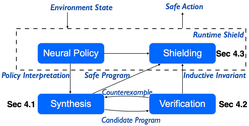
Figure 2. The Framework of Our Approach.

Framework. We construct a policy interpretation mechanism to enable verification, inspired by prior work on imitation learning (Schaal, 1999; Ross et al., 2011) and interpretable machine learning (Verma et al., 2018; Bastani et al., 2018). Fig. 2 depicts the high-level framework of our approach. Our idea is to synthesize a deterministic policy program from a neural policy $\pi_{\mathbf{w}}$, approximating $\pi_{\mathbf{w}}$ (which we call an oracle) with a simpler structural program $\cal{P}$. Like $\pi_{\mathbf{w}}$, $\cal{P}$ takes as input a system state and generates a control action $a$. To this end, ${\cal P}$ is simulated in the environment used to train the neural policy $\pi_{\mathbf{w}}$, to collect feasible states. Guided by $\pi_{\mathbf{w}}$’s actions on such collected states, $\cal{P}$ is further improved to resemble $\pi_{\mathbf{w}}$.

The goal of the synthesis procedure is to search for a deterministic program $\cal{P}^{*}$ satisfying both (1) a quantitative specification such that it bears reasonably close resemblance to its oracle so that allowing it to serve as a potential substitute is a sensible notion, and (2) a desired logical safety property such that when in operation the unsafe states defined in the environment $\cal{C}$ cannot be reached. Formally,

(1) $$\cal{P}^{*}=\operatorname*{arg\,max}_{\cal{P}\in\text{Safe}(\cal{C},\llbracket\cal{H}\rrbracket)}d(\pi_{\mathbf{w}},\cal{P},\cal{C})$$

where $d(\pi_{\mathbf{w}},\cal{P},\cal{C})$ measures proximity of $\cal{P}$ with its neural oracle in an environment $\cal{C}$; $\llbracket\cal{H}\rrbracket$ defines a search space for $\cal{P}$ with prior knowledge on the shape of target deterministic programs; and, $\text{Safe}(\cal{C},\llbracket\cal{H}\rrbracket)$ restricts the solution space to a set of safe programs. A program $\cal{P}$ is safe if the safety of the transition system $\cal{C}[\cal{P}]$, the deployment of $\cal{P}$ in the environment $\cal{C}$, can be formally verified.

The novelty of our approach against prior work on neural policy interpretation (Verma et al., 2018; Bastani et al., 2018) is thus two-fold:

1. We bake in the concept of safety and formal safety verification into the synthesis of a deterministic program from a neural policy as depicted in Fig. 2. If a candidate program is not safe, we rely on a counterexample-guided inductive synthesis loop to improve our synthesis outcome to enforce the safety conditions imposed by the environment.

2. We allow ${\cal P}$ to operate in tandem with the high-performing neural policy. ${\cal P}$ can be viewed as capturing an inductive invariant of the state transition system, which can be used as a shield to describe a boundary of safe states within which the neural policy is free to make optimal control decisions. If the system is about to be driven out of this safety boundary, the synthesized program is used to take an action that is guaranteed to stay within the space subsumed by the invariant. By allowing the synthesis procedure to treat the neural policy as an oracle, we constrain the search space of feasible programs to be those whose actions reside within a proximate neighborhood of actions undertaken by the neural policy.

Synthesis. Reducing a complex neural policy to a simpler yet safe deterministic program is possible because we do not require other properties from the oracle; specifically, we do not require that the deterministic program precisely mirrors the performance of the neural policy. For example, experiments described in (Rajeswaran et al., 2017) show that while a linear-policy controlled robot can effectively stand up, it is unable to learn an efficient walking gait, unlike a sufficiently-trained neural policy. However, if we just care about the safety of the neural network, we posit that a linear reduction can be sufficiently expressive to describe necessary safety constraints. Based on this hypothesis, for our inverted pendulum example, we can explore a linear program space from which a deterministic program $\cal{P}_{\theta}$ can be drawn expressed in terms of the following program sketch:

⬇

def $\cal{P}$[$\theta_1$, $\theta_2$]($\eta$, $\omega$): return $\theta_1 \eta + \theta_2 \omega$

Here, $\theta=[\theta_{1},\theta_{2}]$ are unknown parameters that need to be synthesized. Intuitively, the program weights the importance of $\eta$ and $\omega$ at a particular state to provide a feedback control action to mitigate the deviation of the inverted pendulum from $(\eta=0^{\circ},\omega=0^{\circ})$.

Our search-based synthesis sets $\theta$ to 0 initially. It runs the deterministic program $\cal{P}_{\theta}$ instead of the oracle neural policy $\pi_{\mathbf{w}}$ within the environment $\cal{C}$ defined in Fig. 1 (in this case, the state transition system represents the differential equation specification of the controller) to collect a batch of trajectories. A run of the state transition system of $\cal{C}[\cal{P}_{\theta}]$ produces a finite trajectory $s_{0},s_{1},\cdots,s_{T}$. We find $\theta$ from the following optimization task that realizes (1):

(2) $$\max_{\theta\in\mathbb{R}^{2}}\mathbb{E}[\Sigma^{T}_{t=0}d(\pi_{\mathbf{w}},\cal{P}_{\theta},s_{t})]$$

where $d(\pi_{\mathbf{w}},\cal{P}_{\theta},s_{t})\equiv\begin{cases}-(\cal{P}_{\theta}(s_{t})-\pi_{\mathbf{w}}(s_{t}))^{2}&s_{t}\notin\cal{S}_{u}\\ -MAX&s_{t}\in\cal{S}_{u}\end{cases}$. This equation aims to search for a program $\cal{P}_{\theta}$ at minimal distance from the neural oracle $\pi_{\mathbf{w}}$ along sampled trajectories, while simultaneously maximizing the likelihood that $\cal{P}_{\theta}$ is safe.

Our synthesis procedure described in Sec. 4.1 is a random search-based optimization algorithm (Matyas, 1965). We sample a new position of $\theta$ iteratively from its hypersphere of a given small radius surrounding the current position of $\theta$ and move to the new position (w.r.t. a learning rate) as dictated by Equation (2). For the running example, our search synthesizes:

⬇

def $\cal{P}$($\eta$, $\omega$): return $-12.05 \eta + -5.87 \omega$

The synthesized program can be used to intuitively interpret how the neural oracle works. For example, if a pendulum with a positive angle $\eta>0$ leans towards the right ($\omega>0$), the controller will need to generate a large negative control action to force the pendulum to move left.

Verification. Since our method synthesizes a deterministic program $\cal{P}$, we can leverage off-the-shelf formal verification algorithms to verify its safety with respect to the state transition system $\cal{C}$ defined in Fig. 1. To ensure that $\cal{P}$ is safe, we must ascertain that it can never transition to an unsafe state, i.e., a state that causes the pendulum to fall. When framed as a formal verification problem, answering such a question is tantamount to discovering an inductive invariant $\varphi$ that represents all safe states over the state transition system:

1. Safe: $\varphi$ is disjoint with all unsafe states $\cal{S}_{u}$,

2. Init: $\varphi$ includes all initial states $\cal{S}_{0}$,

3. Induction: Any state in $\varphi$ transitions to another state in $\varphi$ and hence cannot reach an unsafe state.

Inspired by template-based constraint solving approaches on inductive invariant inference (Gulwani and Tiwari, 2008; Gulwani et al., 2008; Prajna and Jadbabaie, 2004; Kong et al., 2013), the verification algorithm described in Sec. 4.2 uses a constraint solver to look for an inductive invariant in the form of a convex barrier certificate (Prajna and Jadbabaie, 2004) $E(s)\leq 0$ that maps all the states in the (safe) reachable set to non-positive reals and all the states in the unsafe set to positive reals. The basic idea is to identify a polynomial function $E:\mathbb{R}^{n}\rightarrow\mathbb{R}$ such that 1) $E(s)>0$ for any state $s\in\cal{S}_{u}$, 2) $E(s)\leq 0$ for any state $s\in\cal{S}_{0}$, and 3) $E(s^{\prime})-E(s)\leq 0$ for any state $s$ that transitions to $s^{\prime}$ in the state transition system $\cal{C}[\cal{P}]$. The second and third condition collectively guarantee that $E(s)\leq 0$ for any state $s$ in the reachable set, thus implying that an unsafe state in $\cal{S}_{u}$ can never be reached.

Fig. 3(a) draws the discovered invariant in blue for $\cal{C}[\cal{P}]$ given the initial and unsafe states where $\cal{P}$ is the synthesized program for the inverted pendulum system. We can conclude that the safety property is satisfied by the $\cal{P}$ controlled system as all reachable states do not overlap with unsafe states. In case verification fails, our approach conducts a counterexample guided loop (Sec. 4.2) to iteratively synthesize safe deterministic programs until verification succeeds.

Shielding. Keep in mind that a safety proof of a reduced deterministic program of a neural network does not automatically lift to a safety argument of the neural network from which it was derived since the network may exhibit behaviors not fully captured by the simpler deterministic program. To bridge this divide, we propose to recover soundness at runtime by monitoring system behaviors of a neural network in its actual environment (deployment) context.

Fig. 4 depicts our runtime shielding approach with more details given in Sec. 4.3. The inductive invariant $\varphi$ learnt for a deterministic program $\cal{P}$ of a neural network $\pi_{\mathbf{w}}$ can serve as a shield to protect $\pi_{\mathbf{w}}$ at runtime under the environment context and safety property used to synthesize $\cal{P}$. An observation about a current state is sent to both $\pi_{\mathbf{w}}$ and the shield. A high-performing neural network is allowed to take any actions it feels are optimal as long as the next state it proposes is still within the safety boundary formally characterized by the inductive invariant of $\cal{C}[\cal{P}]$. Whenever a neural policy proposes an action that steers its controlled system out of the state space defined by the inductive invariant we have learned as part of deterministic program synthesis, our shield can instead take a safe action proposed by the deterministic program $\cal{P}$. The action given by $\cal{P}$ is guaranteed safe because $\varphi$ defines an inductive invariant of $\cal{C}[\cal{P}]$; taking the action allows the system to stay within the provably safe region identified by $\varphi$. Our shielding mechanism is sound due to formal verification. Because the deterministic program was synthesized using $\pi_{\mathbf{w}}$ as an oracle, it is expected that the shield derived from the program will not frequently interrupt the neural network’s decision, allowing the combined system to perform (close-to) optimally.

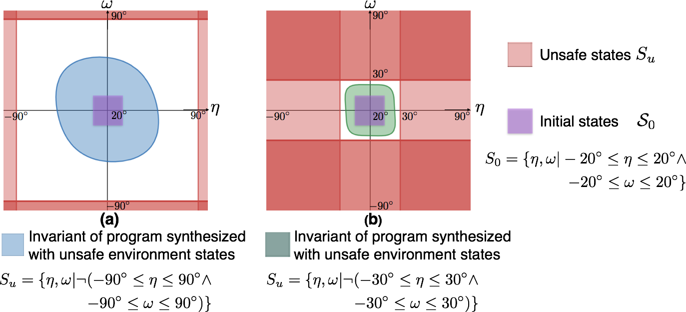
Figure 3. Invariant Inference on Inverted Pendulum.

In the inverted pendulum example, since the $90^{\circ}$ bound given as a safety constraint is rather conservative, we do not expect a well-trained neural network to violate this boundary. Indeed, in Fig. 3(a), even though the inductive invariant of the synthesized program defines a substantially smaller state space than what is permissible, in our simulation results, we find that the neural policy is never interrupted by the deterministic program when governing the pendulum. Note that the non-shaded areas in Fig. 3(a), while appearing safe, presumably define states from which the trajectory of the system can be led to an unsafe state, and would thus not be inductive.

Figure 4. The Framework of Neural Network Shielding.

Our synthesis approach is critical to ensuring safety when the neural policy is used to predict actions in an environment different from the one used during training. Consider a neural network suitably protected by a shield that now operates safely. The effectiveness of this shield would be greatly diminished if the network had to be completely retrained from scratch whenever it was deployed in a new environment which imposes different safety constraints.

In our running example, suppose we wish to operate the inverted pendulum in an environment such as a Segway transporter in which the model is prohibited from swinging significantly and whose angular velocity must be suitably restricted. We might specify the following new constraints on state parameters to enforce these conditions:

$$\cal{S}_{u}:\{(\eta,\omega)\ |\neg(-30^{\circ}<\eta<30^{\circ}\wedge-30^{\circ}<\omega<30^{\circ})\}$$

Because of the dependence of a neural network to the quality of training data used to build it, environment changes that deviate from assumptions made at training-time could result in a costly retraining exercise because the network must learn a new way to penalize unsafe actions that were previously safe. However, training a neural network from scratch requires substantial non-trivial effort, involving fine-grained tuning of training parameters or even network structures.

In our framework, the existing network provides a reasonable approximation to the desired behavior. To incorporate the additional constraints defined by the new environment $\cal{C^{\prime}}$, we attempt to synthesize a new deterministic program $\cal{P^{\prime}}$ for $\cal{C^{\prime}}$, a task based on our experience is substantially easier to achieve than training a new neural network policy from scratch. This new program can be used to protect the original network provided that we can use the aforementioned verification approach to formally verify that $\cal{C^{\prime}}[\cal{P^{\prime}}]$ is safe by identifying a new inductive invariant $\varphi^{\prime}$. As depicted in Fig. 4, we simply build a new shield $\cal{S}^{\prime}$ that is composed of the program $\cal{P}^{\prime}$ and the safety boundary captured by $\varphi^{\prime}$. The shield $\cal{S}^{\prime}$ can ensure the safety of the neural network in the environment context $\cal{C}^{\prime}$ with a strengthened safety condition, despite the fact that the neural network was trained in a different environment context $\cal{C}$.

Fig. 3(b) depicts the new unsafe states in $\cal{C}^{\prime}$ (colored in red). It extends the unsafe range draw in Fig. 3(a) so the inductive invariant learned there is unsafe for the new one. Our approach synthesizes a new deterministic program for which we learn a more restricted inductive invariant depicted in green in Fig. 3(b). To characterize the effectiveness of our shielding approach, we examined 1000 simulation trajectories of this restricted version of the inverted pendulum system, each of which is comprised of 5000 simulation steps with the safety constraints defined by $\cal{C^{\prime}}$. Without the shield $\cal{S}^{\prime}$, the pendulum entered the unsafe region $\cal{S}_{u}$ 41 times. All of these violations were prevented by $\cal{S}^{\prime}$. Notably, the intervention rate of $\cal{S}^{\prime}$ to interrupt the neural network’s decision was extremely low. Out of a total of 5000$\times$1000 decisions, we only observed 414 instances (0.00828%) where the shield interfered with (i.e., overrode) the decision made by the network.

3. Problem Setup

We model the context $\cal{C}$ of a control policy as an environment state transition system $\cal{C}[\cdot]=({X},\cal{A},\cal{S},\cal{S}_{0},\cal{S}_{u},\cal{T}_{t}[\cdot],f,r)$. Note that $\cdot$ is intentionally left open to deploy neural control policies. Here, ${X}$ is a finite set of variables interpreted over the reals $\mathbb{R}$ and $\cal{S}=\mathbb{R}^{X}$ is the set of all valuations of the variables ${X}$. We denote $s\in\cal{S}$ to be an $n$-dimensional environment state and $a\in\cal{A}$ to be a control action where $\cal{A}$ is an infinite set of $m$-dimensional continuous actions that a learning-enabled controller can perform. We use $\cal{S}_{0}\in\cal{S}$ to specify a set of initial environment states and $\cal{S}_{u}\in\cal{S}$ to specify a set of unsafe environment states that a safe controller should avoid. The transition relation $\cal{T}_{t}[\cdot]$ defines how one state transitions to another given an action by an unknown policy. We assume that $\cal{T}_{t}[\cdot]$ is governed by a standard differential equation $f$ defining the relationship between a continuously varying state $s(t)$ and action $a(t)$ and its rate of change $\dot{s}(t)$ over time $t$:

$$\dot{s}(t)=f(s(t),a(t))$$

We assume $f$ is defined by equations of the form: $\mathbb{R}^{n}\times\mathbb{R}^{m}\rightarrow\mathbb{R}^{n}$ such as the example in Fig. 1. In the following, we often omit the time variable $t$ for simplicity. A deterministic neural network control policy $\pi_{\mathbf{w}}:\mathbb{R}^{n}\rightarrow\mathbb{R}^{m}$ parameterized by a set of weight values $\mathbf{w}$ is a function mapping an environment state $s$ to a control action $a$ where

$$a=\pi_{\mathbf{w}}(s)$$

By providing a feedback action, a policy can alter the rate of change of state variables to realize optimal system control.

The transition relation $\cal{T}_{t}[\cdot]$ is parameterized by a control policy $\pi$ that is deployed in $\cal{C}$. We explicitly model this deployment as $\cal{T}_{t}[\pi]$. Given a control policy $\pi_{\mathbf{w}}$, we use $\cal{T}_{t}[\pi_{\mathbf{w}}]:\cal{S}\times\cal{S}$ to specify all possible state transitions allowed by the policy. We assume that a system transitions in discrete time instants $kt$ where $k=0,1,2,\cdots$ and $t$ is a fixed time step ($t>0$). A state $s$ transitions to a next state $s^{\prime}$ after time $t$ with the assumption that a control action $a(\tau)$ at time $\tau$ is a constant between the time period $\tau\in[0,t)$. Using Euler’s method, we discretize the continuous dynamics $f$ with finite difference approximation so it can be used in the discretized transition relation $\cal{T}_{t}[\pi_{\mathbf{w}}]$. Then $\cal{T}_{t}[\pi_{\mathbf{w}}]$ can compute these estimates by the following difference equation:

$$\cal{T}_{t}[\pi_{\mathbf{w}}]:=\{(s,s^{\prime})\ |\ s^{\prime}=s+f(s,\pi_{\mathbf{w}}(s))\times t\}$$

Environment Disturbance. Our model allows bounded external properties (e.g., additional environment-imposed constraints) by extending the definition of change of rate: $\dot{s}=f(s,a)+d$ where $d$ is a vector of random disturbances. We use $d$ to encode environment disturbances in terms of bounded nondeterministic values. We assume that tight upper and lower bounds of $d$ can be accurately estimated at runtime using multivariate normal distribution fitting methods.

Trajectory. A trajectory $h$ of a state transition system $\cal{C}[\pi_{\mathbf{w}}]$ which we denote as $h\in\cal{C}[\pi_{\mathbf{w}}]$ is a sequence of states $s_{0},\cdots,s_{i},s_{i+1},\cdots$ where $s_{0}\in\cal{S}_{0}$ and $(s_{i},s_{i+1})\in\cal{T}_{t}[\pi_{\mathbf{w}}]$ for all $i\geq 0$. We use $C\subseteq\cal{C}[\pi_{\mathbf{w}}]$ to denote a set of trajectories. The reward that a control policy receives on performing an action $a$ in a state $s$ is given by the reward function $r(s,a)$.

Reinforcement Learning. The goal of reinforcement learning is to maximize the reward that can be collected by a neural control policy in a given environment context $\cal{C}$. Such problems can be abstractly formulated as

(3) $$\begin{split}\max_{\mathbf{w}\in\mathbb{R}^{n}}&J(\mathbf{w})\\ J(\mathbf{w})=\mathbb{E}&[r(\pi_{\mathbf{w}})]\end{split}$$

Assume that $s_{0},s_{1},\ldots,s_{T}$ is a trajectory of length $T$ of the state transition system and $r(\pi_{\mathbf{w}})=\lim\limits_{T\to\infty}\Sigma^{T}_{k=0}r(s_{k},\pi_{\mathbf{w}}(s_{k}))$ is the cumulative reward achieved by the policy $\pi_{\mathbf{w}}$ from this trajectory. Thus this formulation uses simulations of the transition system with finite length rollouts to estimate the expected cumulative reward collected over $T$ time steps and aim to maximize this reward. Reinforcement learning assumes polices are expressible in some executable structure (e.g. a neural network) and allows samples generated from one policy to influence the estimates made for others. The two main approaches for reinforcement learning are value function estimation and direct policy search. We refer readers to (Li, 2017) for an overview.

Safety Verification. Since reinforcement learning only considers finite length rollouts, we wish to determine if a control policy is safe to use under an infinite time horizon. Given a state transition system, the safety verification problem is concerned with verifying that no trajectories contained in $\cal{S}$ starting from an initial state in $\cal{S}_{0}$ reach an unsafe state in $\cal{S}_{u}$. However, a neural network is a representative of a class of deep and sophisticated models that challenges the capability of the state-of-the-art verification techniques. This level of complexity is exacerbated in our work because we consider the long term safety of a neural policy deployed within a nontrivial environment context $\cal{C}$ that in turn is described by a complex infinite-state transition system.

4. Verification Procedure

To verify a neural network control policy $\pi_{\mathbf{w}}$ with respect to an environment context $\cal{C}$, we first synthesize a deterministic policy program $\cal{P}$ from the neural policy. We require that $\cal{P}$ both (a) broadly resembles its neural oracle and (b) additionally satisfies a desired safety property when it is deployed in $\cal{C}$. We conjecture that a safety proof of $\cal{C}[\cal{P}]$ is easier to construct than that of $\cal{C}[\pi_{\mathbf{w}}]$. More importantly, we leverage the safety proof of $\cal{C}[\cal{P}]$ to ensure the safety of $\cal{C}[\pi_{\mathbf{w}}]$.

4.1. Synthesis

Fig. 5 defines a search space for a deterministic policy program $\cal{P}$ where $E$ and $\varphi$ represent the basic syntax of (polynomial) program expressions and inductive invariants, respectively. Here $v$ ranges over a universe of numerical constants, $x$ represents variables, and $\oplus$ is a basic operator including $+$ and $\times$. A deterministic program $\cal{P}$ also features conditional statements using $\varphi$ as branching predicates.

We allow the user to define a sketch (Solar-Lezama, 2008, 2009) to describe the shape of target policy programs using the grammar in Fig. 5. We use $\cal{P}[\theta]$ to represent a sketch where $\theta$ represents unknowns that need to be filled-in by the synthesis procedure. We use $\cal{P}_{\theta}$ to represent a synthesized program with known values of $\theta$. Similarly, the user can define a sketch of an inductive invariant $\varphi[\cdot]$ that is used (in Sec. 4.2) to learn a safety proof to verify a synthesized program $\cal{P}_{\theta}$.

$$E ::=v\ |\ x\ |\ \oplus(E_{1},\ldots,E_{k})$$

$$\varphi ::=E\leq 0$$

$$\cal{P} ::=\text{\bf return }\ E\ |\ \text{\bf if}\ \varphi\ \text{\bf then}\ \text{\bf return}\ E\ \text{\bf else}\ \cal{P}$$

Figure 5. Syntax of the Policy Programming Language.

We do not require the user to explicitly define conditional statements in a program sketch. Our synthesis algorithm uses verification counterexamples to lazily add branch predicates $\varphi$ under which a program performs different computations depending on whether $\varphi$ evaluates to true or false. The end user simply writes a sketch over basic expressions. For example, a sketch that defines a family of linear function over a collection of variables can be expressed as:

(4) $${\cal P}[\theta](X)::=\text{\bf return}\ \theta_{1}x_{1}+\theta_{2}x_{2}+\cdots+\theta_{n}x_{n}+\theta_{n+1}$$

Here $X=(x_{1},x_{2},\cdots)$ are system variables in which the coefficient constants $\theta=(\theta_{1},\theta_{2},\cdots)$ are unknown.

The goal of our synthesis algorithm is to find unknown values of $\theta$ that maximize the likelihood that $\cal{P}_{\theta}$ resembles the neural oracle $\pi_{\mathbf{w}}$ while still being a safe program with respect to the environment context $\cal{C}$:

(5) $$\theta^{*}=\operatorname*{arg\,max}_{\theta\in\mathbb{R}^{n+1}}d(\pi_{\mathbf{w}},\cal{P}_{\theta},\cal{C})$$

where $d$ measures the distance between the outputs of the estimate program $\cal{P}_{\theta}$ and the neural policy $\pi_{\mathbf{w}}$ subject to safety constraints. To avoid the computational complexity that arises if we consider a solution to this equation analytically as an optimization problem, we instead approximate $d(\pi_{\mathbf{w}},\cal{P}_{\theta},\cal{C})$ by randomly sampling a set of trajectories $C$ that are encountered by $\cal{P}_{\theta}$ in the environment state transition system $\cal{C}[\cal{P}_{\theta}]$:

$$d(\pi_{\mathbf{w}},\cal{P}_{\theta},\cal{C})\approx d(\pi_{\mathbf{w}},\cal{P}_{\theta},C)\ s.t.\ C\subseteq\cal{C}[\cal{P}_{\theta}]$$

We estimate $\theta^{*}$ using these sampled trajectories $C$ and define:

$$d(\pi_{\mathbf{w}},\cal{P}_{\theta},C)=\sum_{h\in C}d(\pi_{\mathbf{w}},\cal{P}_{\theta},h)$$

Since each trajectory $h\in C$ is a finite rollout $s_{0},\ldots,s_{T}$ of length $T$, we have:

$$d(\pi_{\mathbf{w}},\cal{P}_{\theta},h)=\sum_{t=0}^{T}\begin{cases}-\left\lVert(\cal{P}_{\theta}(s_{t})-\pi_{\mathbf{w}}(s_{t}))\right\rVert&s_{t}\notin\cal{S}_{u}\\ -MAX&s_{t}\in\cal{S}_{u}\end{cases}$$

where $\left\lVert\cdot\right\rVert$ is a suitable norm. As illustrated in Sec. 2.2, we aim to minimize the distance between a synthesized program $\cal{P}_{\theta}$ from a sketch space and its neural oracle along sampled trajectories encountered by $\cal{P}_{\theta}$ in the environment context but put a large penalty on states that are unsafe.

1 $\theta$ $\leftarrow$ $\mathbf{0}$;

2 do

3       Sample $\delta$ from a zero mean Gaussian vector;

4       Sample a set of trajectories $C_{1}$ using $\cal{C}[\cal{P}_{\theta+\nu\delta}]$;

5       Sample a set of trajectories $C_{2}$ using $\cal{C}[\cal{P}_{\theta-\nu\delta}]$;

6       $\theta\leftarrow\theta+{\alpha}[\frac{d(\pi_{\mathbf{w}},\cal{P}_{\theta+\nu\delta},C_{1})-d(\pi_{\mathbf{w}},\cal{P}_{\theta-\nu\delta},C_{2})}{\nu}]\delta$;

7      

8while $\theta$ is not converged;

return $\cal{P}_{\theta}$

Algorithm 1 Synthesize ($\pi_{\mathbf{w}}$, $\cal{P}[\theta]$, $\cal{C}[\cdot]$)

Random Search. We implement the idea encoded in equation (5) in Algorithm 1 that depicts the pseudocode of our policy interpretation approach. It take as inputs a neural policy, a policy program sketch parameterized by $\theta$, and an environment state transition system and outputs a synthesized policy program $\cal{P}_{\theta}$.

An efficient way to solve equation (5) is to directly perturb $\theta$ in the search space by adding random noise and then update $\theta$ based on the effect on this perturbation (Matyas, 1965). We choose a direction uniformly at random on the sphere in parameter space, and then optimize the goal function along this direction. To this end, in line 3 of Algorithm 1, we sample Gaussian noise $\delta$ to be added to policy parameters $\theta$ in both directions where $\nu$ is a small positive real number. In line 4 and line 5, we sample trajectories $C_{1}$ and $C_{2}$ from the state transition systems obtained by running the perturbed policy program $\cal{P}_{\theta+\nu\delta}$ and $\cal{P}_{\theta-\nu\delta}$ in the environment context $\cal{C}$.

We evaluate the proximity of these two policy programs to the neural oracle and, in line 6 of Algorithm 1, to improve the policy program, we also optimize equation (5) by updating $\theta$ with a finite difference approximation along the direction:

(6) $$\theta\leftarrow\theta+{\alpha}[\frac{d(\cal{P}_{\theta+\nu\delta},\pi_{\mathbf{w}},C_{1})-d(\cal{P}_{\theta-\nu\delta},\pi_{\mathbf{w}},C_{2})}{\nu}]\delta$$

where $\alpha$ is a predefined learning rate. Such an update increment corresponds to an unbiased estimator of the gradient of $\theta$ (Nesterov and Spokoiny, 2017; Mania et al., 2018) for equation (5). The algorithm iteratively updates $\theta$ until convergence.

4.2. Verification

A synthesized policy program $\cal{P}$ is verified with respect to an environment context given as an infinite state transition system defined in Sec. 3: $\cal{C}[\cal{P}]=({X},\cal{A},\cal{S},\cal{S}_{0},\cal{S}_{u},\cal{T}_{t}[\cal{P}],f,r)$. Our verification algorithm learns an inductive invariant $\varphi$ over the transition relation $\cal{T}_{t}[\cal{P}]$ formally proving that all possible system behaviors are encapsulated in $\varphi$ and $\varphi$ is required to be disjoint with all unsafe states $\cal{S}_{u}$.

We follow template-based constraint solving approaches for inductive invariant inference (Gulwani and Tiwari, 2008; Gulwani et al., 2008; Prajna and Jadbabaie, 2004; Kong et al., 2013) to discover this invariant. The basic idea is to identify a function $E:\mathbb{R}^{n}\rightarrow\mathbb{R}$ that serves as a ”barrier” (Gulwani and Tiwari, 2008; Prajna and Jadbabaie, 2004; Kong et al., 2013) between reachable system states (evaluated to be nonpositive by $E$), and unsafe states (evaluated positive by $E$). Using the invariant syntax in Fig. 5, the user can define an invariant sketch

(7) $$\varphi[c](X)::=E[c](X)\leq 0$$

over variables $X$ and $c$ unknown coefficients intended to be synthesized. Fig. 5 carefully restricts that an invariant sketch $E[c]$ can only be postulated as a polynomial function as there exist efficient SMT solvers (De Moura and Bjørner, 2008) and constraint solvers (Legat et al., 2018) for nonlinear polynomial reals. Formally, assume real coefficients $c=(c_{0},\cdots,c_{p})$ are used to parameterize $E[c]$ in an affine manner:

$$E[c](X)=\Sigma^{p}_{i=0}c_{i}b_{i}(X)$$

where the $b_{i}(X)$’s are some monomials in variables $X$. As a heuristic, the user can simply determine an upper bound on the degree of $E[c]$, and then include all monomials whose degrees are no greater than the bound in the sketch. Large values of the bound enable verification of more complex safety conditions, but impose greater demands on the constraint solver; small values capture coarser safety properties, but are easier to solve.

Example 4.1 (label=ex1).

Consider the inverted pendulum system in Sec. 2.2. To discover an inductive invariant for the transition system, the user might choose to define an upper bound of 4, which results in the following polynomial invariant sketch: $\varphi[c](\eta,\omega)::=E[c](\eta,\omega)\leq 0$ where

$$E[c](\eta,\omega)=c_{0}\eta^{4}+c_{1}\eta^{3}\omega+c_{2}\eta^{2}\omega^{2}+c_{3}\eta\omega^{3}+c_{4}\omega^{4}+c_{5}\eta^{3}+\cdots+c_{p}$$

The sketch includes all monomials over $\eta$ and $\omega$, whose degrees are no greater than 4. The coefficients $c=[c_{0},\cdots,c_{p}]$ are unknown and need to be synthesized.

To synthesize these unknowns, we require that $E[c]$ must satisfy the following verification conditions:

(8) $$\forall(s)\in\cal{S}_{u} E[c](s)>0$$

(9) $$\forall(s)\in\cal{S}_{0} E[c](s)\leq 0$$

(10) $$\forall(s,s^{\prime})\in\cal{T}_{t}[\cal{P}] E[c](s^{\prime})-E[c](s)\leq 0.$$

We claim that $\varphi::=E[c](x)\leq 0$ defines an inductive invariant because verification condition (9) ensures that any initial state $s_{0}\in S_{0}$ satisfies $\varphi$ since $E[c](s_{0})\leq 0$; verification condition (10) asserts that along the transition from a state $s\in\varphi$ (so $E[c](s)\leq 0$) to a resulting state $s^{\prime}$, $E[c]$ cannot become positive so $s^{\prime}$ satisfies $\varphi$ as well. Finally, according to verification condition (8), $\varphi$ does not include any unsafe state $s_{u}\in\cal{S}_{u}$ as $E[c](s_{u})$ is positive.

Verification conditions (8) (9) (10) are polynomials over reals. Synthesizing unknown coefficients can be left to an SMT solver (De Moura and Bjørner, 2008) after universal quantifiers are eliminated using a variant of Farkas Lemma as in (Gulwani and Tiwari, 2008). However, observe that $E[c]$ is convex. We can gain efficiency by finding unknown coefficients $c$ using off-the-shelf convex constraint solvers following (Prajna and Jadbabaie, 2004). Encoding verification conditions (8) (9) (10) as polynomial inequalities, we search $c$ that can prove non-negativity of these constraints via an efficient and convex sum of squares programming solver (Legat et al., 2018). Additional technical details are provided in the supplementary material (Zhu et al., 2018).

Counterexample-guided Inductive Synthesis (CEGIS). Given the environment state transition system $\cal{C}[\cal{P}]$ deployed with a synthesized program $\cal{P}$, the verification approach above can compute an inductive invariant over the state transition system or tell if there is no feasible solution in the given set of candidates. Note however that the latter does not necessarily imply that the system is unsafe.

Since our goal is to learn a safe deterministic program from a neural network, we develop a counterexample guided inductive program synthesis approach. A CEGIS algorithm in our context is challenging because safety verification is necessarily incomplete, and may not be able to produce a counterexample that serves as an explanation for why a verification attempt is unsuccessful.

We solve the incompleteness challenge by leveraging the fact that we can simultaneously synthesize and verify a program. Our CEGIS approach is given in Algorithm 2. A counterexample is an initial state on which our synthesized program is not yet proved safe. Driven by these counterexamples, our algorithm synthesizes a set of programs from a sketch along with the conditions under which we can switch from from one synthesized program to another.

1 policies $\leftarrow$ $\emptyset$;

2 covers $\leftarrow$ $\emptyset$;

3 while $\cal{C}.\cal{S}_{0}$ $\not\subseteq$ covers do

4       search $s_{0}$ such that $s_{0}\in\cal{C}.\cal{S}_{0}\wedge s_{0}\notin{\sf covers}$;

5       $r^{*}$ $\leftarrow$ Diameter($\cal{C}.\cal{S}_{0}$);

6       do

7             $\phi_{bound}$ $\leftarrow$ $\{s\ |\ s\in\{s_{0}-r^{*},s_{0}+r^{*}\}\}$;

8             $\cal{\tilde{C}}$ $\leftarrow$ $\cal{C}$ where $\cal{\tilde{C}}.\cal{S}_{0}=(\cal{C}.\cal{S}_{0}\cap\phi_{bound})$;

9             $\theta$ $\leftarrow$ Synthesize($\pi_{\mathbf{w}}$, $\cal{P}[\theta]$, $\cal{\tilde{C}}[\cdot]$);

10             $\varphi$ $\leftarrow$ Verify($\cal{\tilde{C}}[\cal{P}_{\theta}]$);

11             if $\varphi$ is False then

12                   $r^{*}$ $\leftarrow$ $r^{*}/2$;

13                  

14             else

15                   covers $\leftarrow$ covers $\cup$ $\{s\ |\ \varphi(s)\}$;

16                   policies $\leftarrow$ policies $\cup$ ($\cal{P}_{\theta}$, $\varphi$);

17                   break;

18                  

19            

20      while True;

21 end while

return policies

Algorithm 2 CEGIS ($\pi_{\mathbf{w}}$, $\cal{P}[\theta]$, $\cal{C}[\cdot]$)

Algorithm 2 takes as input a neural policy $\pi_{\mathbf{w}}$, a program sketch $\cal{P}[\theta]$ and an environment context $\cal{C}$. It maintains synthesized policy programs in policies in line 1, each of which is inductively verified safe in a partition of the universe state space that is maintained in covers in line 2. For soundness, the state space covered by such partitions must be able to include all initial states, checked in line 3 of Algorithm 2 by an SMT solver. In the algorithm, we use $\cal{C}.\cal{S}_{0}$ to access a field of $\cal{C}$ such as its initial state space.

The algorithm iteratively samples a counterexample initial state $s_{0}$ that is currently not covered by covers in line 4. Since covers is empty at the beginning, this choice is uniformly random initially; we synthesize a presumably safe policy program in line 9 of Algorithm 2 that resembles the neural policy $\pi_{\mathbf{w}}$ considering all possible initial states $\cal{S}_{0}$ of the given environment model $\cal{C}$, using Algorithm 1.

If verification fails in line 11, our approach simply reduces the initial state space, hoping that a safe policy program is easier to synthesize if only a subset of initial states are considered. The algorithm in line 12 gradually shrinks the radius $r^{*}$ of the initial state space around the sampled initial state $s_{0}$. The synthesis algorithm in the next iteration synthesizes and verifies a candidate using the reduced initial state space. The main idea is that if the initial state space is shrunk to a restricted area around $s_{0}$ but a safety policy program still cannot be found, it is quite possible that either $s_{0}$ points to an unsafe initial state of the neural oracle or the sketch is not sufficiently expressive.

If verification at this stage succeeds with an inductive invariant $\varphi$, a new policy program $\cal{P}_{\theta}$ is synthesized that can be verified safe in the state space covered by $\varphi$. We add the inductive invariant and the policy program into covers and policies in line 14 and 15 respectively and then move to another iteration of counterexample-guided synthesis. This iterative synthesize-and-verify process continues until the entire initial state space is covered (line 3 to 18). The output of Algorithm 2 is $[({\cal{P}_{\theta}}_{1},\varphi_{1}),({\cal{P}_{\theta}}_{2},\varphi_{2}),\cdots]$ that essentially defines conditional statements in a synthesized program performing different actions depending on whether a specified invariant condition evaluates to true or false.

Theorem 4.2.

If $CEGIS(\pi_{w},\cal{P}[\theta],\cal{C}[\cdot])=[({\cal{P}_{\theta}}_{1},\varphi_{1}),({\cal{P}_{\theta}}_{2},\\ \varphi_{2}),\cdots]$ (as defined in Algorithm 2), then the deterministic program $\cal{P}$:

⬇

$\lambda X$.if $\varphi_1(X)$: return ${\cal{P}_\theta}_1(X)$ else if $\varphi_2(X)$: return ${\cal{P}_\theta}_2(X)$ $\cdots$

is safe in the environment $\cal{C}$ meaning that $\varphi_{1}\vee\varphi_{2}\vee\cdots$ is an inductive invariant of $\cal{C}[\cal{P}]$ proving that $\cal{C}.\cal{S}_{u}$ is unreachable.

Figure 6. CEGIS for Verifiable Reinforcement Learning.

Example 4.3.

We illustrate the proposed counterexample guided inductive synthesis method by means of a simple example, the Duffing oscillator (Jordan and Smith, 1987), a nonlinear second-order environment. The transition relation of the environment system $\cal{C}$ is described with the differential equation:

$$\dot{x}=y$$

$$\dot{y}=-0.6y-x-x^{3}+a$$

where $x,y$ are the state variables and $a$ the continuous control action given by a well-trained neural feedback control policy $\pi$ such that $a=\pi(x,y)$. The control objective is to regulate the state to the origin from a set of initial states $\cal{C}.\cal{S}_{0}:\{x,y|-2.5\leq x\leq 2.5\wedge-2\leq y\leq 2\}$. To be safe, the controller must be able to avoid a set of unsafe states $\cal{C}.\cal{S}_{u}:\{x,y|\ \neg(-5\leq x\leq 5\wedge-5\leq y\leq 5)\}$. Given a program sketch as in the pendulum example, that is $\cal{P}[\theta](x,y)::=\theta_{1}x+\theta_{2}y$, the user can ask the constraint solver to reason over a small (say 4) order polynomial invariant sketch for a synthesized program as in Example LABEL:ex1.

Algorithm 2 initially samples an initial state $s$ as $\{x=-0.46,y=-0.36\}$ from $\cal{S}_{0}$. The inner do-while loop of the algorithm can discover a sub-region of initial states in the dotted box of Fig. 6(a) that can be leveraged to synthesize a verified deterministic policy $\cal{P}_{1}(x,y)::=0.39x-1.41y$ from the sketch. We also obtain an inductive invariant showing that the synthesized policy can always maintain the controller within the invariant set drawn in purple in Fig. 6(a): $\varphi_{1}\equiv 20.9x^{4}+2.9x^{3}y+1.4x^{2}y^{2}+0.4xy^{3}+29.6x^{3}+20.1x^{2}y+11.3xy^{2}+1.6y^{3}+25.2x^{2}+39.2xy+53.7y^{2}-680\leq 0$.

This invariant explains why the initial state space used for verification does not include the entire $\cal{C}.\cal{S}_{0}$: a counterexample initial state $s^{\prime}=\{x=2.249,y=2\}$ is not covered by the invariant for which the synthesized policy program above is not verified safe. The CEGIS loop in line 3 of Algorithm 2 uses $s^{\prime}$ to synthesize another deterministic policy $\cal{P}_{2}(x,y)::=0.88x-2.34y$ from the sketch whose learned inductive invariant is depicted in blue in Fig. 2(b): $\varphi_{2}\equiv 12.8x^{4}+0.9x^{3}y-0.2x^{2}y^{2}-5.9x^{3}-1.5xy^{2}-0.3y^{3}+2.2x^{2}+4.7xy+40.4y^{2}-619\leq 0$. Algorithm 2 then terminates because $\varphi_{1}\vee\varphi_{2}$ covers $\cal{C}.\cal{S}_{0}$. Our system interprets the two synthesized deterministic policies as the following deterministic program $\cal{P}_{\mathit{oscillator}}$ using the syntax in Fig. 5:

⬇

def $\cal{P}_{\mathit{oscillator}}\ (x, y)$:

if $20.9x^4 + 2.9x^3y + 1.4x^2y^2 + \cdots + 53.7y^2 - 680 \le 0$: # $\color{red} \varphi_1$

return $0.39x -1.41y$

else if $12.8x^4 + 0.9x^3y - 0.2x^2y^2 + \cdots + 40.4y^2 - 619 \le 0$: # $\color{red} \varphi_2$

return $0.88x -2.34y$

else abort # unsafe

Neither of the two deterministic policies enforce safety by themselves on all initial states but do guarantee safety when combined together because by construction, $\varphi=\varphi_{1}\vee\varphi_{2}$ is an inductive invariant of $\cal{P}_{\mathit{oscillator}}$ in the environment $\cal{C}$.

Although Algorithm 2 is sound, it may not terminate as $r^{*}$ in the algorithm can become arbitrarily small and there is also no restriction on the size of potential counterexamples. Nonetheless, our experimental results indicate that the algorithm performs well in practice.

4.3. Shielding

A safety proof of a synthesized deterministic program of a neural network does not automatically lift to a safety argument of the neural network from which it was derived since the network may exhibit behaviors not captured by the simpler deterministic program. To bridge this divide, we recover soundness at runtime by monitoring system behaviors of a neural network in its environment context by using the synthesized policy program and its inductive invariant as a shield. The pseudo-code for using a shield is given in Algorithm 3. In line 1 of Algorithm 3, for a current state $s$, we use the state transition system of our environment context model to predict the next state $s^{\prime}$. If $s^{\prime}$ is not within $\varphi$, we are unsure whether entering $s^{\prime}$ would inevitably make the system unsafe as we lack a proof that the neural oracle is safe. However, we do have a guarantee that if we follow the synthesized program $\cal{P}$, the system would stay within the safety boundary defined by $\varphi$ that Algorithm 2 has formally proved. We do so in line 3 of Algorithm 3, using $\cal{P}$ and $\varphi$ as shields, intervening only if necessary so as to restrict the shield from unnecessarily intervening the neural policy.

5. Experimental Results

Table 1. Experimental Results on Deterministic Program Synthesis, Verification, and Shielding.

		Neural Network			Deterministic Program as Shield				Performance
Benchmarks	Vars	Size	Training	Failures	Size	Synthesis	Overhead	Interventions	NN	Program
Satellite	2	$240\times 200$	957s	0	1	160s	3.37%	0	5.7	9.7
DCMotor	3	$240\times 200$	944s	0	1	68s	2.03%	0	11.9	12.2
Tape	3	$240\times 200$	980s	0	1	42s	2.63%	0	3.0	3.6
Magnetic Pointer	3	$240\times 200$	992s	0	1	85s	2.92%	0	8.3	8.8
Suspension	4	$240\times 200$	960s	0	1	41s	8.71%	0	4.7	6.1
Biology	3	$240\times 200$	978s	0	1	168s	5.23%	0	2464	2599
DataCenter Cooling	3	$240\times 200$	968s	0	1	168s	4.69%	0	14.6	40.1
Quadcopter	2	$300\times 200$	990s	182	2	67s	6.41%	185	7.2	9.8
Pendulum	2	$240\times 200$	962s	60	3	1107s	9.65%	65	44.2	58.6
CartPole	4	$300\times 200$	990s	47	4	998s	5.62%	1799	681.3	1912.6
Self-Driving	4	$300\times 200$	990s	61	1	185s	4.66%	236	145.9	513.6
Lane Keeping	4	$240\times 200$	895s	36	1	183s	8.65%	64	375.3	643.5
4-Car platoon	8	$500\times 400\times 300$	1160s	8	4	609s	3.17%	8	7.6	9.6
8-Car platoon	16	$500\times 400\times 300$	1165s	40	1	1217s	6.05%	1080	38.5	55.4
Oscillator	18	$240\times 200$	1023s	371	1	618s	21.31%	93703	693.5	1135.3

We have applied our framework on a number of challenging control- and cyberphysical-system benchmarks. We consider the utility of our approach for verifying the safety of trained neural network controllers. We use the deep policy gradient algorithm (Lillicrap et al., 2016) for neural network training, the Z3 SMT solver (De Moura and Bjørner, 2008) to check convergence of the CEGIS loop, and the Mosek constraint solver (ApS, 2018) to generate inductive invariants of synthesized programs from a sketch. All of our benchmarks are verified using the program sketch defined in equation (4) and the invariant sketch defined in equation (7). We report simulation results on our benchmarks over 1000 runs (each run consists of 5000 simulation steps). Each simulation time step is fixed 0.01 second. Our experiments were conducted on a standard desktop machine consisting of Intel(R) Core(TM) i7-8700 CPU cores and 64GB memory.

1 Predict $s^{\prime}$ such that $(s,s^{\prime})\in\cal{C}[\pi_{\mathbf{w}}].\cal{T}_{t}(s)$;

2 if $\varphi(s^{\prime})$ then  return $\pi_{\mathbf{w}}(s)$ ;

3 else  return $\cal{P}(s)$ ;

Algorithm 3 Shield ($s$, $\cal{C}[\pi_{\mathbf{w}}]$, $\cal{P}$, $\varphi$)

Case Study on Inverted Pendulum.

We first give more details on the evaluation result of our running example, the inverted pendulum. Here we consider a more restricted safety condition that deems the system to be unsafe when the pendulum’s angle is more than 23^∘ from the origin (i.e., significant swings are further prohibited). The controller is a 2 hidden-layer neural model ($240\times 200$). Our tool interprets the neural network as a program containing three conditional branches:

⬇

def $\cal{P}\ (\eta, \omega)$:

if $17533\eta^4 + 13732\eta^3\omega + 3831\eta^2\omega^2 - 5472\eta\omega^3 + 8579\omega^4 + 6813\eta^3 +$

$9634\eta^2\omega + 3947\eta\omega^2 - 120\omega^3 + 1928\eta^2 + 1915\eta\omega + 1104\omega^2 - 313 \le 0$:

return $-17.28176866\eta -10.09441768\omega$

else if $2485\eta^4 + 826\eta^3\omega - 351\eta^2\omega^2 + 581\eta\omega^3 + 2579\omega^4 + 591\eta^3 +$

$9\eta^2\omega + 243\eta\omega^2 - 189\omega^3 + 484\eta^2 + 170\eta\omega + 287\omega^2 - 82 \le 0$:

return $-17.34281984x -10.73944835y$

else if $115496\eta^4 + 64763\eta^3\omega + 85376\eta^2\omega^2 + 21365\eta\omega^3 + 7661\omega^4 -$

$111271\eta^3 - 54416\eta^2\omega - 66684\eta\omega^2 - 8742\omega^3 + 33701\eta^2 +$

$11736\eta\omega + 12503\omega^2 - 1185 \le 0$:

return $-25.78835525\eta -16.25056971\omega$

else abort

Over 1000 simulation runs, we found 60 unsafe cases when running the neural controller alone. Importantly, running the neural controller in tandem with the above verified and synthesized program can prevent all unsafe neural decisions. There were only with 65 interventions from the program on the neural network. Our results demonstrate that CEGIS is important to ensure a synthesized program is safe to use. We report more details including synthesis times below.

One may ask why we do not directly learn a deterministic program to control the device (without appealing to the neural policy at all), using reinforcement learning to synthesize its unknown parameters. Even for an example as simple as the inverted pendulum, our discussion above shows that it is difficult (if not impossible) to derive a single straight-line (linear) program that is safe to control the system. Even for scenarios in which a straight-line program suffices, using existing RL methods to directly learn unknown parameters in our sketches may still fail to obtain a safe program. For example, we considered if a linear control policy can be learned to (1) prevent the pendulum from falling down (2) and require a pendulum control action to be strictly within the range $[-1,1]$ (e.g., operating the controller in an environment with low power constraints). We found that despite many experiments on tuning learning rates and rewards, directly training a linear control program to conform to this restriction with either reinforcement learning (e.g. policy gradient) or random search (Mania et al., 2018) was unsuccessful because of undesirable overfitting. In contrast, neural networks work much better for these RL algorithms and can be used to guide the synthesis of a deterministic program policy. Indeed, by treating the neural policy as an oracle, we were able to quickly discover a straight-line linear deterministic program that in fact satisfies this additional motion constraint.

Safety Verification.

Our verification results are given in Table 1. In the table, Vars represents the number of variables in a control system - this number serves as a proxy for application complexity; Size the number of neurons in hidden layers of the network; the Training time for the network; and, its Failures, the number of times the network failed to satisfy the safety property in simulation. The table also gives the Size of a synthesized program in term of the number of polices found by Algorithm 2 (used to generate conditional statements in the program); its Synthesis time; the Overhead of our approach in terms of the additional cost (compared to the non-shielded variant) in running time to use a shield; and, the number of Interventions, the number of times the shield was invoked across all simulation runs. We also report performance gap between of a shield neural policy (NN) and a purely programmatic policy (Program), in terms of the number of steps on average that a controlled system spends in reaching a steady state of the system (i.e., a convergence state).

The first five benchmarks are linear time-invariant control systems adapted from (Fan et al., 2018). The safety property is that the reach set has to be within a safe rectangle. Benchmark Biology defines a minimal model of glycemic control in diabetic patients such that the dynamics of glucose and insulin interaction in the blood system are defined by polynomials (Bergman et al., 1985). For safety, we verify that the neural controller ensures that the level of plasma glucose concentration is above a certain threshold. Benchmark DataCenter Cooling is a model of a collection of three server racks each with their own cooling devices and they also shed heat to their neighbors. The safety property is that a learned controller must keep the data center below a certain temperature. In these benchmarks, the cost to query the network oracle constitutes the dominant time for generating the safety shield in these benchmarks. Given the simplicity of these benchmarks, the neural network controllers did not violate the safety condition in our trials, and moreover there were no interventions from the safety shields that affected performance.

The next three benchmarks Quadcopter, (Inverted) Pendulum and Cartpole are selected from classic control applications and have more sophisticated safety conditions. We have discussed the inverted pendulum example at length earlier. The Quadcopter environment tests whether a controlled quadcopter can realize stable flight. The environment of Cartpole consists of a pole attached to an unactuated joint connected to a cart that moves along a frictionless track. The system is unsafe when the pole’s angle is more than 30^∘ from being upright or the cart moves by more than 0.3 meters from the origin. We observed safety violations in each of these benchmarks that were eliminated using our verification methodology. Notably, the number of interventions is remarkably low, as a percentage of the overall number of simulation steps.

Benchmark Self-driving defines a single car navigation problem. The neural controller is responsible for preventing the car from veering into canals found on either side of the road. Benchmark Lane Keeping models another safety-related car-driving problem. The neural controller aims to maintain a vehicle between lane markers and keep it centered in a possibly curved lane. The curvature of the road is considered as a disturbance input. Environment disturbances of such kind can be conservatively specified in our model, accounting for noise and unmodeled dynamics. Our verification approach supports these disturbances (verification condition (10)). Benchmarks $n$-Car platoon model multiple ($n$) vehicles forming a platoon, maintaining a safe relative distance among one another (Schürmann and Althoff, 2017). Each of these benchmarks exhibited some number of violations that were remediated by our verification methodology. Benchmark Oscillator consists of a two-dimensional switched oscillator plus a 16-order filter. The filter smoothens the input signals and has a single output signal. We verify that the output signal is below a safe threshold. Because of the model complexity of this benchmark, it exhibited significantly more violations than the others. Indeed, the neural-network controlled system often oscillated between the safe and unsafe boundary in many runs. Consequently, the overhead in this benchmark is high because a large number of shield interventions was required to ensure safety. In other words, the synthesized shield trades performance for safety to guarantee that the threshold boundary is never violated.

For all benchmarks, our tool successfully generated safe interpretable deterministic programs and inductive invariants as shields. When a neural controller takes an unsafe action, the synthesized shield correctly prevents this action from executing by providing an alternative provable safe action proposed by the verified deterministic program. In term of performance, Table 1 shows that a shielded neural policy is a feasible approach to drive a controlled system into a steady state. For each of the benchmarks studied, the programmatic policy is less performant than the shielded neural policy, sometimes by a factor of two or more (e.g., Cartpole, Self-Driving, and Oscillator). Our result demonstrates that executing a neural policy in tandem with a program distilled from it can retain performance, provided by the neural policy, while maintaining safety, provided by the verified program.

Although our synthesis algorithm does not guarantee convergence to the global minimum when applied to nonconvex RL problems, the results given in Table 1 indicate that our algorithm can often produce high-quality control programs, with respect to a provided sketch, that converge reasonably fast. In some of our benchmarks, however, the number of interventions are significantly higher than the number of neural controller failures, e.g., 8-Car platoon and Oscillator. However, the high number of interventions is not primarily because of non-optimality of the synthesized programmatic controller. Instead, inherent safety issues in the neural network models are the main culprit that triggers shield interventions. In 8-Car platoon, after corrections made by our deterministic program, the neural model again takes an unsafe action in the next execution step so that the deterministic program has to make another correction. It is only after applying a number of such shield interventions that the system navigates into a part of the state space that can be safely operated on by the neural model. For this benchmark, all system states where there occur shield interventions are indeed unsafe. We also examined the unsafe simulation runs made by executing the neural controller alone in Oscillator. Among the large number of shield interventions (as reflected in Table 1), 74% of them are effective and indeed prevent an unsafe neural decision. Ineffective interventions in Oscillator are due to the fact that, when optimizing equation (5), a large penalty is given to unsafe states, causing the synthesized programmatic policy to weigh safety more than proximity when there exist a large number of unsafe neural decisions.

Suitable Sketches.

Providing a suitable sketch may need domain knowledge. To help the user more easily tune the shape of a sketch, our approach provides algorithmic support by not requiring conditional statements in a program sketch and syntactic sugar, i.e., the user can simply provide an upper bound on the degree of an invariant sketch.

Table 2. Experimental Results on Tuning Invariant Degrees. TO means that an adequate inductive invariant cannot be found within 2 hours.

Benchmarks	Degree	Verification	Interventions	Overhead
Pendulum	2	TO	-	-
	4	22.6s	40542	7.82%
	8	23.6s	30787	8.79%
Self-Driving	2	TO	-	-
	4	24s	128851	6.97%
	8	25.1s	123671	26.85%
8-Car-platoon	2	172.9s	43952	8.36%
	4	540.2s	37990	9.19%
	8	TO	-	-

Our experimental results are collected using the invariant sketch defined in equation (7) and we chose an upper bound of 4 on the degree of all monomials included in the sketch. Recall that invariants may also be used as conditional predicates as part of a synthesized program. We adjust the invariant degree upper bound to evaluate its effect in our synthesis procedure. The results are given in Table 2.

Table 3. Experimental Results on Handling Environment Changes.

		Neural Network		Deterministic Program as Shield
Benchmarks	Environment Change	Size	Failures	Size	Synthesis	Overhead	Shield Interventions
Cartpole	Increased Pole length by 0.15m	$1200\times 900$	3	1	239s	2.91%	8
Pendulum	Increased Pendulum mass by 0.3kg	$1200\times 900$	77	1	581s	8.11%	8748
Pendulum	Increased Pendulum length by 0.15m	$1200\times 900$	76	1	483s	6.53%	7060
Self-driving	Added an obstacle that must be avoided	$1200\times 900$	203	1	392s	8.42%	108320

Generally, high-degree invariants lead to fewer interventions because they tend to be more permissive than low-degree ones. However, high-degree invariants take more time to synthesize and verify. This is particularly true for high-dimension models such as 8-Car platoon. Moreover, although high-degree invariants tend to have fewer interventions, they have larger overhead. For example, using a shield of degree 8 in the Self-Driving benchmark caused an overhead of 26.85%. This is because high-degree polynomial computations are time-consuming. On the other hand, an insufficient degree upper bound may not be permissive enough to obtain a valid invariant. It is, therefore, essential to consider the tradeoff between overhead and permissiveness when choosing the degree of an invariant.

Handling Environment Changes.

We consider the effectiveness of our tool when previously trained neural network controllers are deployed in environment contexts different from the environment used for training. Here we consider neural network controllers of larger size (two hidden layers with $1200\times 900$ neurons) than in the above experiments. This is because we want to ensure that a neural policy is trained to be near optimal in the environment context used for training. These larger networks were in general more difficult to train, requiring at least 1500 seconds to converge.

Our results are summarized in Table 3. When the underlying environment sightly changes, learning a new safety shield takes substantially shorter time than training a new network. For Cartpole, we simulated the trained controller in a new environment by increasing the length of the pole by 0.15 meters. The neural controller failed 3 times in our 1000 episode simulation; the shield interfered with the network operation only 8 times to prevent these unsafe behaviors. The new shield was synthesized in 239s significantly faster than retraining a new neural network for the new environment. For (Inverted) Pendulum, we deployed the trained neural network in an environment in which the pendulum’s mass is increased by 0.3kg. The neural controller exhibits noticeably higher failure rates than in the previous experiment; we were able to synthesize a safety shield adapted to this new environment in 581 seconds that prevented these violations. The shield intervened with the operation of the network only 8.7 number of times per episode. Similar results were observed when we increased the pendulum’s length by 0.15m. For Self-driving, we additionally required the car to avoid an obstacle. The synthesized shield provided safe actions to ensure collision-free motion.

6. Related Work

Verification of Neural Networks. While neural networks have historically found only limited application in safety- and security-related contexts, recent advances have defined suitable verification methodologies that are capable of providing stronger assurance guarantees. For example, Reluplex (Katz et al., 2017) is an SMT solver that supports linear real arithmetic with ReLU constraints and has been used to verify safety properties in a collision avoidance system. AI² (Gehr et al., 2018; Mirman et al., 2018) is an abstract interpretation tool that can reason about robustness specifications for deep convolutional networks. Robustness verification is also considered in (Bastani et al., 2016; Huang et al., 2017). Systematic testing techniques such as (Tian et al., 2018; Sun et al., 2018; Wicker et al., 2018) are designed to automatically generate test cases to increase a coverage metric, i.e., explore different parts of neural network architecture by generating test inputs that maximize the number of activated neurons. These approaches ignore effects induced by the actual environment in which the network is deployed. They are typically ineffective for safety verification of a neural network controller over an infinite time horizon with complex system dynamics. Unlike these whitebox efforts that reason over the architecture of the network, our verification framework is fully blackbox, using a network only as an oracle to learn a simpler deterministic program. This gives us the ability to reason about safety entirely in terms of the synthesized program, using a shielding mechanism derived from the program to ensure that the neural policy can only explore safe regions.

Safe Reinforcement Learning. The machine learning community has explored various techniques to develop safe reinforcement machine learning algorithms in contexts similar to ours, e.g., (Moldovan and Abbeel, 2012; Turchetta et al., 2016). In some cases, verification is used as a safety validation oracle (Akametalu et al., 2014a; Berkenkamp et al., 2017). In contrast to these efforts, our inductive synthesis algorithm can be freely incorporated into any existing reinforcement learning framework and applied to any legacy machine learning model. More importantly, our design allows us to synthesize new shields from existing ones, without requiring retraining of the network, under reasonable changes to the environment.

Syntax-Guided Synthesis for Machine Learning. An important reason underlying the success of program synthesis is that sketches of the desired program (Solar-Lezama, 2009, 2008), often provided along with example data, can be used to effectively restrict a search space and allow users to provide additional insight about the desired output (Alur et al., 2015). Our sketch based inductive synthesis approach is a realization of this idea applicable to continuous and infinite state control systems central to many machine learning tasks. A high-level policy language grammar is used in our approach to constrain the shape of possible synthesized deterministic policy programs. Our program parameters in sketches are continuous, because they naturally fit continuous control problems. However, our synthesis algorithm (line 9 of Algorithm 2) can call a derivate-free random search method (which does not require the gradient or its approximative finite difference) for synthesizing functions whose domain is disconnected, (mixed-) integer, or non-smooth. Our synthesizer thus may be applied to other domains that are not continuous or differentiable like most modern program synthesis algorithms (Solar-Lezama, 2009, 2008).

In a similar vein, recent efforts on interpretable machine learning generate interpretable models such as program code (Verma et al., 2018) or decision trees (Bastani et al., 2018) as output, after which traditional symbolic verification techniques can be leveraged to prove program properties. Our approach novelly ensures that only safe programs are synthesized via a CEGIS procedure and can provide safety guarantees on the original high-performing neural networks via invariant inference. A detailed comparison was provided on page 2.2.

Controller Synthesis. Random search (Matyas, 1965) has long been utilized as an effective approach for controller synthesis. In (Mania et al., 2018), several extensions of random search have been proposed that substantially improve its performance when applied to reinforcement learning. However, (Mania et al., 2018) learns a single linear controller that we found to be insufficient to guarantee safety for our benchmarks in our experience. We often need to learn a program that involves a family of linear controllers conditioned on different input spaces to guarantee safety. The novelty of our approach is that it can automatically synthesize programs with conditional statements by need, which is critical to ensure safety.

In Sec. 5, linear sketches were used in our experiments for shield synthesis. LQR-Tree based approaches such as (Tedrake, 2009) can synthesize a controller consisting of a set of linear quadratic regulator (LQR (Dorato et al., 1994)) controllers each applicable in a different portion of the state space. These approaches focus on stability while our approach primarily addresses safety. In our experiments, we observed that because LQR does not take safe/unsafe regions into consideration, synthesized LQR controllers can regularly violate safety constraints.

Runtime Shielding. Shield synthesis has been used in runtime enforcement for reactive systems (Bloem et al., 2015; Könighofer et al., 2017). Safety shielding in reinforcement learning was first introduced in (Alshiekh et al., 2018). Because their verification approach is not symbolic, however, it can only work over finite discrete state and action systems. Since states in infinite state and continuous action systems are not enumerable, using these methods requires the end user to provide a finite abstraction of complex environment dynamics; such abstractions are typically too coarse to be useful (because they result in too much over-approximation), or otherwise have too many states to be analyzable (Fan et al., 2018). Indeed, automated environment abstraction tools such as (Filippidis et al., 2016) often take hours even for simple 4-dimensional systems. Our approach embraces the nature of infinity in control systems by learning a symbolic shield from an inductive invariant for a synthesized program that includes an infinite number of environment states under which the program can be guaranteed to be safe. We therefore believe our framework provides a more promising verification pathway for machine learning in high-dimensional control systems. In general, these efforts focused on shielding of discrete and finite systems with no obvious generalization to effectively deal with continuous and infinite systems that our approach can monitor and protect. Shielding in continuous control systems was introduced in (Akametalu et al., 2014b; Gillula and Tomlin, 2012). These approaches are based on HJ reachability (Hamilton-Jacobi Reachability (Bansal et al., 2017)). However, current formulations of HJ reachability are limited to systems with approximately five dimensions, making high-dimensional system verification intractable. Unlike their least restrictive control law framework that decouples safety and learning, our approach only considers state spaces that a learned controller attempts to explore and is therefore capable of synthesizing safety shields even in high dimensions.

7. Conclusions

This paper presents an inductive synthesis-based toolchain that can verify neural network control policies within an environment formalized as an infinite-state transition system. The key idea is a novel synthesis framework capable of synthesizing a deterministic policy program based on an user-given sketch that resembles a neural policy oracle and simultaneously satisfies a safety specification using a counterexample-guided synthesis loop. Verification soundness is achieved at runtime by using the learned deterministic program along with its learned inductive invariant as a shield to protect the neural policy, correcting the neural policy’s action only if the chosen action can cause violation of the inductive invariant. Experimental results demonstrate that our approach can be used to realize fully trustworthy reinforcement learning systems with low overhead.

References

- (1)
- Ahmadi et al. (2018) M. Ahmadi, C. Rowley, and U. Topcu. 2018. Control-Oriented Learning of Lagrangian and Hamiltonian Systems. In American Control Conference.
- Akametalu et al. (2014a) Anayo K. Akametalu, Shahab Kaynama, Jaime F. Fisac, Melanie Nicole Zeilinger, Jeremy H. Gillula, and Claire J. Tomlin. 2014a. Reachability-based safe learning with Gaussian processes. In 53rd IEEE Conference on Decision and Control, CDC 2014. 1424–1431.
- Akametalu et al. (2014b) Anayo K. Akametalu, Shahab Kaynama, Jaime F. Fisac, Melanie Nicole Zeilinger, Jeremy H. Gillula, and Claire J. Tomlin. 2014b. Reachability-based safe learning with Gaussian processes. In 53rd IEEE Conference on Decision and Control, CDC 2014, Los Angeles, CA, USA, December 15-17, 2014. 1424–1431.
- Alshiekh et al. (2018) Mohammed Alshiekh, Roderick Bloem, Rüdiger Ehlers, Bettina Könighofer, Scott Niekum, and Ufuk Topcu. 2018. Safe Reinforcement Learning via Shielding. AAAI (2018).
- Alur et al. (2015) Rajeev Alur, Rastislav Bodík, Eric Dallal, Dana Fisman, Pranav Garg, Garvit Juniwal, Hadas Kress-Gazit, P. Madhusudan, Milo M. K. Martin, Mukund Raghothaman, Shambwaditya Saha, Sanjit A. Seshia, Rishabh Singh, Armando Solar-Lezama, Emina Torlak, and Abhishek Udupa. 2015. Syntax-Guided Synthesis. In Dependable Software Systems Engineering. NATO Science for Peace and Security Series, D: Information and Communication Security, Vol. 40. IOS Press, 1–25.
- ApS (2018) MOSEK ApS. 2018. The mosek optimization software. http://www.mosek.com
- Bansal et al. (2017) Somil Bansal, Mo Chen, Sylvia Herbert, and Claire J Tomlin. 2017. Hamilton-Jacobi Reachability: A Brief Overview and Recent Advances. (2017).
- Bastani et al. (2016) Osbert Bastani, Yani Ioannou, Leonidas Lampropoulos, Dimitrios Vytiniotis, Aditya V. Nori, and Antonio Criminisi. 2016. Measuring Neural Net Robustness with Constraints. In Proceedings of the 30th International Conference on Neural Information Processing Systems (NIPS’16). 2621–2629.
- Bastani et al. (2018) Osbert Bastani, Yewen Pu, and Armando Solar-Lezama. 2018. Verifiable Reinforcement Learning via Policy Extraction. CoRR abs/1805.08328 (2018).
- Bergman et al. (1985) Richard N Bergman, Diane T Finegood, and Marilyn Ader. 1985. Assessment of insulin sensitivity in vivo. Endocrine reviews 6, 1 (1985), 45–86.
- Berkenkamp et al. (2017) Felix Berkenkamp, Matteo Turchetta, Angela P. Schoellig, and Andreas Krause. 2017. Safe Model-based Reinforcement Learning with Stability Guarantees. In Advances in Neural Information Processing Systems 30: Annual Conference on Neural Information Processing Systems 2017. 908–919.
- Bloem et al. (2015) Roderick Bloem, Bettina Könighofer, Robert Könighofer, and Chao Wang. 2015. Shield Synthesis: - Runtime Enforcement for Reactive Systems. In Tools and Algorithms for the Construction and Analysis of Systems - 21st International Conference, TACAS 2015. 533–548.
- De Moura and Bjørner (2008) Leonardo De Moura and Nikolaj Bjørner. 2008. Z3: An Efficient SMT Solver. In Proceedings of the Theory and Practice of Software, 14th International Conference on Tools and Algorithms for the Construction and Analysis of Systems (TACAS’08/ETAPS’08). 337–340.
- Dorato et al. (1994) Peter Dorato, Vito Cerone, and Chaouki Abdallah. 1994. Linear-Quadratic Control: An Introduction. Simon & Schuster, Inc., New York, NY, USA.
- Fan et al. (2018) Chuchu Fan, Umang Mathur, Sayan Mitra, and Mahesh Viswanathan. 2018. Controller Synthesis Made Real: Reach-Avoid Specifications and Linear Dynamics. In Computer Aided Verification - 30th International Conference, CAV 2018. 347–366.
- Filippidis et al. (2016) Ioannis Filippidis, Sumanth Dathathri, Scott C. Livingston, Necmiye Ozay, and Richard M. Murray. 2016. Control design for hybrid systems with TuLiP: The Temporal Logic Planning toolbox. In 2016 IEEE Conference on Control Applications, CCA 2016. 1030–1041.
- Gehr et al. (2018) Timon Gehr, Matthew Mirman, Dana Drachsler-Cohen, Petar Tsankov, Swarat Chaudhuri, and Martin T. Vechev. 2018. AI2: Safety and Robustness Certification of Neural Networks with Abstract Interpretation. In 2018 IEEE Symposium on Security and Privacy, SP 2018. 3–18.
- Gillula and Tomlin (2012) Jeremy H. Gillula and Claire J. Tomlin. 2012. Guaranteed Safe Online Learning via Reachability: tracking a ground target using a quadrotor. In IEEE International Conference on Robotics and Automation, ICRA 2012, 14-18 May, 2012, St. Paul, Minnesota, USA. 2723–2730.
- Gulwani et al. (2008) Sumit Gulwani, Saurabh Srivastava, and Ramarathnam Venkatesan. 2008. Program Analysis As Constraint Solving. In Proceedings of the 29th ACM SIGPLAN Conference on Programming Language Design and Implementation (PLDI ’08). 281–292.
- Gulwani and Tiwari (2008) Sumit Gulwani and Ashish Tiwari. 2008. Constraint-based approach for analysis of hybrid systems. In International Conference on Computer Aided Verification. 190–203.
- Huang et al. (2017) Xiaowei Huang, Marta Kwiatkowska, Sen Wang, and Min Wu. 2017. Safety Verification of Deep Neural Networks. In CAV (1) (Lecture Notes in Computer Science), Vol. 10426. 3–29.
- Jordan and Smith (1987) Dominic W Jordan and Peter Smith. 1987. Nonlinear ordinary differential equations. (1987).
- Katz et al. (2017) Guy Katz, Clark W. Barrett, David L. Dill, Kyle Julian, and Mykel J. Kochenderfer. 2017. Reluplex: An Efficient SMT Solver for Verifying Deep Neural Networks. In Computer Aided Verification - 29th International Conference, CAV 2017. 97–117.
- Kong et al. (2013) Hui Kong, Fei He, Xiaoyu Song, William N. N. Hung, and Ming Gu. 2013. Exponential-Condition-Based Barrier Certificate Generation for Safety Verification of Hybrid Systems. In Proceedings of the 25th International Conference on Computer Aided Verification (CAV’13). 242–257.
- Könighofer et al. (2017) Bettina Könighofer, Mohammed Alshiekh, Roderick Bloem, Laura Humphrey, Robert Könighofer, Ufuk Topcu, and Chao Wang. 2017. Shield Synthesis. Form. Methods Syst. Des. 51, 2 (Nov. 2017), 332–361.
- Legat et al. (2018) Benoît Legat, Chris Coey, Robin Deits, Joey Huchette, and Amelia Perry. 2017 (accessed Nov 16, 2018). Sum-of-squares optimization in Julia. https://www.juliaopt.org/meetings/mit2017/legat.pdf
- Li (2017) Yuxi Li. 2017. Deep Reinforcement Learning: An Overview. CoRR abs/1701.07274 (2017).
- Lillicrap et al. (2016) Timothy P. Lillicrap, Jonathan J. Hunt, Alexander Pritzel, Nicolas Heess, Tom Erez, Yuval Tassa, David Silver, and Daan Wierstra. 2016. Continuous control with deep reinforcement learning. In 4th International Conference on Learning Representations, ICLR 2016, San Juan, Puerto Rico, May 2-4, 2016, Conference Track Proceedings.
- Mania et al. (2018) Horia Mania, Aurelia Guy, and Benjamin Recht. 2018. Simple random search of static linear policies is competitive for reinforcement learning. In Advances in Neural Information Processing Systems 31. 1800–1809.
- Matyas (1965) J Matyas. 1965. Random optimization. Automation and Remote Control 26, 2 (1965), 246–253.
- Mirman et al. (2018) Matthew Mirman, Timon Gehr, and Martin T. Vechev. 2018. Differentiable Abstract Interpretation for Provably Robust Neural Networks. In Proceedings of the 35th International Conference on Machine Learning, ICML 2018. 3575–3583.
- Moldovan and Abbeel (2012) Teodor Mihai Moldovan and Pieter Abbeel. 2012. Safe Exploration in Markov Decision Processes. In Proceedings of the 29th International Coference on International Conference on Machine Learning (ICML’12). 1451–1458.
- Nesterov and Spokoiny (2017) Yurii Nesterov and Vladimir Spokoiny. 2017. Random Gradient-Free Minimization of Convex Functions. Found. Comput. Math. 17, 2 (2017), 527–566.
- Prajna and Jadbabaie (2004) Stephen Prajna and Ali Jadbabaie. 2004. Safety Verification of Hybrid Systems Using Barrier Certificates. In Hybrid Systems: Computation and Control, 7th International Workshop, HSCC 2004. 477–492.
- Rajeswaran et al. (2017) Aravind Rajeswaran, Kendall Lowrey, Emanuel Todorov, and Sham M. Kakade. 2017. Towards Generalization and Simplicity in Continuous Control. In Advances in Neural Information Processing Systems 30: Annual Conference on Neural Information Processing Systems 2017. 6553–6564.
- Ross et al. (2011) Stéphane Ross, Geoffrey J. Gordon, and Drew Bagnell. 2011. A Reduction of Imitation Learning and Structured Prediction to No-Regret Online Learning. In Proceedings of the Fourteenth International Conference on Artificial Intelligence and Statistics, AISTATS 2011. 627–635.
- Ruan et al. (2018) Wenjie Ruan, Xiaowei Huang, and Marta Kwiatkowska. 2018. Reachability Analysis of Deep Neural Networks with Provable Guarantees. In Proceedings of the Twenty-Seventh International Joint Conference on Artificial Intelligence, IJCAI 2018. 2651–2659.
- Schaal (1999) Stefan Schaal. 1999. Is imitation learning the route to humanoid robots? Trends in cognitive sciences 3, 6 (1999), 233–242.
- Schürmann and Althoff (2017) Bastian Schürmann and Matthias Althoff. 2017. Optimal control of sets of solutions to formally guarantee constraints of disturbed linear systems. In 2017 American Control Conference, ACC 2017. 2522–2529.
- Silver et al. (2014) David Silver, Guy Lever, Nicolas Heess, Thomas Degris, Daan Wierstra, and Martin Riedmiller. 2014. Deterministic Policy Gradient Algorithms. In Proceedings of the 31st International Conference on International Conference on Machine Learning - Volume 32. I–387–I–395.
- Solar-Lezama (2008) Armando Solar-Lezama. 2008. Program Synthesis by Sketching. Ph.D. Dissertation. Berkeley, CA, USA. Advisor(s) Bodik, Rastislav.
- Solar-Lezama (2009) Armando Solar-Lezama. 2009. The Sketching Approach to Program Synthesis. In Proceedings of the 7th Asian Symposium on Programming Languages and Systems (APLAS ’09). 4–13.
- Sun et al. (2018) Youcheng Sun, Min Wu, Wenjie Ruan, Xiaowei Huang, Marta Kwiatkowska, and Daniel Kroening. 2018. Concolic Testing for Deep Neural Networks. In Proceedings of the 33rd ACM/IEEE International Conference on Automated Software Engineering (ASE 2018). 109–119.
- Tedrake (2009) Russ Tedrake. 2009. LQR-trees: Feedback motion planning on sparse randomized trees. In Robotics: Science and Systems V, University of Washington, Seattle, USA, June 28 - July 1, 2009.
- Tian et al. (2018) Yuchi Tian, Kexin Pei, Suman Jana, and Baishakhi Ray. 2018. DeepTest: Automated Testing of Deep-neural-network-driven Autonomous Cars. In Proceedings of the 40th International Conference on Software Engineering (ICSE ’18). 303–314.
- Turchetta et al. (2016) Matteo Turchetta, Felix Berkenkamp, and Andreas Krause. 2016. Safe Exploration in Finite Markov Decision Processes with Gaussian Processes. In Proceedings of the 30th International Conference on Neural Information Processing Systems (NIPS’16). 4312–4320.
- Verma et al. (2018) Abhinav Verma, Vijayaraghavan Murali, Rishabh Singh, Pushmeet Kohli, and Swarat Chaudhuri. 2018. Programmatically Interpretable Reinforcement Learning. In Proceedings of the 35th International Conference on Machine Learning, ICML 2018. 5052–5061.
- Wicker et al. (2018) Matthew Wicker, Xiaowei Huang, and Marta Kwiatkowska. 2018. Feature-Guided Black-Box Safety Testing of Deep Neural Networks. In Tools and Algorithms for the Construction and Analysis of Systems - 24th International Conference, TACAS 2018. 408–426.
- Zhu et al. (2018) He Zhu, Zikang Xiong, Stephen Magill, and Suresh Jagannathan. 2018. An Inductive Synthesis Framework for Verifiable Reinforcement Learning. Technical Report. Galois, Inc. http://herowanzhu.github.io/herowanzhu.github.io/VerifiableLearning.pdf