Inference-Based Resource Allocation
for Multi-Cell Backscatter Sensor Networks

Abstract

This work studies inference-based resource allocation in ultra low-power, large-scale backscatter sensor networks (BSNs). Several ultra-low cost and power sensor devices (tags) are illuminated by a carrier and reflect the measured information towards a wireless core that uses conventional Marconi radio technology. The development of multi-cell BSNs requires few multi-antenna cores and several low-cost scatter radio devices, targeting at maximum possible coverage. The average signal-to-interference-plus-noise ratio (SINR) of maximum-ratio combining (MRC) and zero-forcing (ZF) linear detectors is found and harnessed for frequency sub-channel allocation at tags, exploiting long-term SINR information. The resource allocation problem is formulated as an integer programming optimization problem and solved through the Max-Sum message-passing algorithm. The proposed algorithm is fully parallelizable and adheres to simple message-passing update rules, requiring mainly addition and comparison operations. In addition, the convergence to the optimal solution is attained within very few iteration steps. Judicious simulation study reveals that ZF detector is more suitable for large scale BSNs, capable to cancel out the intra-cell interference. It is also found that the proposed algorithm offers at least an order of magnitude decrease in execution time compared to conventional convex optimization methods.

I Introduction

Backscatter sensor networks (BSNs) have emerged as a promising technology for ultra low-cost, large-scale wireless sensor networking and relevant internet-of-things (IoT) applications [1, 2, 3]. A multi-cell BSN consists of a few interrogators (or cores) that act as fusion centers and tags/sensors that are responsible for measuring environmental quantities, and transmitting the sensed information towards the cores. Cores use the conventional Marconi radio technology with front-ends consisting of active filters, mixers, and amplifiers. On the other hand, tags utilize scatter radio technology and rely on the reflection principle: Cores emit a continuous sinusoidal wave that illuminates the tags in their vicinity, which in turn use backscattering, i.e., they modulate information onto the incident signal by alternating a radio frequency (RF) transistor switch according to the sensed data.

Current BSNs are extremely power-limited due to the round-trip nature of backscatter communication; even for free-space propagation loss, received power decays with the forth-power as a function of core-to-tag distance [4]. Especially for passive tags, the maximum achieved range is on the order of a few meters – far from the required standards of large-scale, low-cost, ubiquitous sensing applications. As a result, increasing the coverage, or equivalently, increasing core-to-tag communication range, is of principle importance in low-cost, low-power BSNs. To overcome the limited range issues, prior art in backscatter communications has proposed: (a) semi-passive tags and (b) power-limited modulation at tags, such as minimum-shift keying (MSK) [2] or frequency-shift keying (FSK) [5]. Especially, FSK is ideal for power-limited and low-bit rate communications and in conjunction with semi-passive tags, offers promising core-to-tag ranges, on the order of hundreds of meters [6, 7]. In contrast to passive tags, semi-passive tags are powered through an external power source, e.g., a battery, or a super-capacitor, or other ambient sources (e.g., solar or RF or their combination).

This work examines a multi-cell BSN architecture with joint time-frequency multiple-access. A measurement phase is considered to assess signal-to-interference-plus-noise ratio (SINR) information at the tags in the BSN. The frequency sub-channel allocation at tags changes during the measurement phase and the goal at each core is to assess the average SINR for each pair of neighboring tag-frequency sub-channel. Subsequently, resource allocation based on a maximization of a specific metric, involving a function of estimated average SINR is applied to find the optimal frequency assignment.

Using the above multi-cell BSN framework, the contributions of this work are summarized as follows:

• For zero-forcing (ZF) and maximum ratio combining (MRC) multiuser detection techniques, the average received SINR is extracted and subsequently harnessed to produce a generic formulation for resource allocation in BSNs. The formulated problem is attacked with a message-passing inference algorithm with simple update rules and convergence to the desired solution within very few lightweight steps. The proposed algorithm is an instance of the Max-Sum algorithm.

• Judicious simulation study corroborates theoretical findings, showing that the proposed Max-Sum algorithm offers the same optimal performance with classic convex optimization methods with reduced computational cost, measured in terms of execution time in large-scale BSNs.

Notation: The set of real, complex, natural, and binary numbers is denoted $\mathds{R}$, $\mathds{C}$, $\mathds{N}$, and $\mathds{B}$, respectively. Operators $(\cdot)^{*}$, $\Re\{\cdot\}$, $(\cdot)^{\top}$ , $(\cdot)^{\mathsf{H}}$, and $(\cdot)^{\dagger}$ take the conjugate, real part, transpose, conjugate transpose, and pseudo-inverse respectively. $\mathbf{I}_{N}$ and $\mathbf{0}_{N}$ ($\mathbf{1}_{N}$) represent the $N\times N$ identity matrix and the all-zeros (all-ones) vector of size $N$, respectively. $\mathcal{CN}(\boldsymbol{\mu},\boldsymbol{\Sigma})$ denotes the proper complex Gaussian distribution with mean $\boldsymbol{\mu}$ and covariance matrix $\boldsymbol{\Sigma}$. $\mathbb{E}[\cdot]$ denotes the expectation operator.

II Wireless Scatter Radio System Model

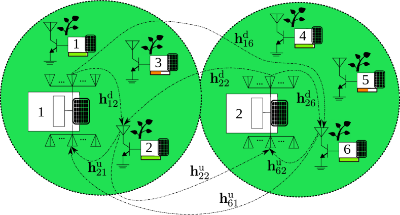
Figure 1: A multi-cell BSN with $B=2$ cores and $K=6$ tags.

We consider a static multi-cell backscatter sensor network (BSN) consisting of $B$ cores and $K$ sensors/tags; an example is given in Fig. 1. Each core is a Marconi radio with separate transmit and receive antennas, e.g., a software define radio (SDR) reader. It is assumed that each core has $N_{\rm T}$ transmit and $N_{\rm R}$ receive antennas. The set of all cores and tags is given by the sets $\mathcal{B}\triangleq\{1,2,\ldots,B\}$ and $\mathcal{K}\triangleq\{1,2,\ldots,K\}$, respectively. There exist at total $C$ orthogonal frequency sub-carriers (or sub-channels) $\left\{\mathtt{f}^{(1)},\mathtt{f}^{(2)},\ldots,\mathtt{f}^{(C)}\right\}$, given in an ascending order, indexed by set $\mathcal{C}\triangleq\{1,2,\ldots,C\}$. The distance between core $b$ and tag $k$ is denoted $\mathsf{d}_{kb}$.

Due to relatively small symbol rate, $1/T$, delay spread is considered negligible, and thus, frequency non-selective (flat) fading channel [8] is assumed across core-to-tag links $(b,k)$ and tag-to-core links $(k,b)$, $b\in\mathcal{B}$, $k\in\mathcal{K}$. For outdoor environments, it is customary to assume strong line-of-site components, and thus, the baseband complex channel responses for downlink $(b,k)$ and uplink $(k,b)$ are, respectively, given by:

$$\mathbf{h}_{bk}^{\rm d}\sim\mathcal{CN}\left(\sqrt{\frac{\kappa_{bk}^{\rm d}}{\kappa_{bk}^{\rm d}+1}}\sigma_{bk}\mathbf{e}_{bk}^{\rm d},\frac{\sigma_{bk}^{2}}{\kappa_{bk}^{\rm d}+1}\mathbf{I}_{N_{\rm T}}\right),$$ (1)

$$\mathbf{h}_{kb}^{\rm u}\sim\mathcal{CN}\left(\sqrt{\frac{\kappa_{kb}^{\rm u}}{\kappa_{kb}^{\rm u}+1}}\sigma_{kb}\mathbf{e}_{kb}^{\rm u},\frac{\sigma_{kb}^{2}}{\kappa_{kb}^{\rm u}+1}\mathbf{I}_{N_{\rm R}}\right),$$ (2)

where $\kappa_{bk}^{\rm d}$ and $\kappa_{kb}^{\rm u}$ denote the ratio between the power in the direct path and the power in the scattered paths of core-to-tag link $(b,k)$ and tag-to-core link $(k,b)$, respectively. $\mathbf{e}_{bk}^{\rm d}$ and $\mathbf{e}_{kb}^{\rm u}$ are the antenna steering vectors, depending, respectively, on the angle-of-departure (AoD) and angle-of-arrival (AoA) between core $b$ and tag $k$. $\frac{1}{N_{\rm T}}\mathbb{E}[\|\mathbf{h}_{bk}^{\rm d}\|_{2}^{2}]=\sigma_{bk}^{2}$ and $\frac{1}{N_{\rm R}}\mathbb{E}[\|\mathbf{h}_{kb}^{\rm u}\|_{2}^{2}]=\sigma_{kb}^{2}$ denote the normalized channel powers of core-to-tag link $(b,k)$ and tag-to-core link $(k,b)$, respectively. Both downlink $\{\mathbf{h}_{bk}^{\rm d}\}_{(b,k)\in\mathcal{B}\times\mathcal{K}}$ and uplink $\{\mathbf{h}_{kb}^{\rm u}\}_{(b,k)\in\mathcal{B}\times\mathcal{K}}$ channel gains are assumed uncorrelated of each other and across any pair $(b,k)$, changing independently every $T_{\rm coh}$ seconds, where $T_{\rm coh}$ is the channel coherence time. The normalized channel powers depend on large-scale path-gain (inverse of path-loss) which is assumed the same for links $(b,k)$ and $(k,b)$, i.e., $\sigma_{bk}=\sigma_{kb}$.

When a tag $k\in\mathcal{K}$ reflects information, it backscatters a packet of $M$ symbols, where each symbol within a packet takes values $\{\pm 1\}$. $M_{\rm tr}$ symbols form a preamble, dedicated for training and the rest $M_{\rm d}=M-M_{\rm tr}$ are data symbols. The set of available training sequences $\mathcal{X}_{\rm tr}=\left\{\mathbf{x}^{(1)},\mathbf{x}^{(2)},\ldots,\mathbf{x}^{(M_{\rm tr})}\right\}\subset\{\pm 1\}^{M_{\rm tr}}$, i.e., set $\mathcal{X}_{\rm tr}$ contains $M_{\rm tr}$ sequences, each of dimension $M_{\rm tr}$. The sequences in set $\mathcal{X}_{\rm tr}$ are orthogonal, i.e., $\left(\mathbf{x}^{(m)}\right)^{\top}\mathbf{x}^{(m^{\prime})}=0$, for $m\neq m^{\prime}$. The training sequence assigned to a tag $k$ has been decided a-priori and is assumed fixed. In a practical scenario, to reduce the training interference, the same training sequence has to be reused across tags that are far apart. Let $\mathcal{M}_{\rm tr}\triangleq\{1,2,\ldots,M_{\rm tr}\}$ and $\mathcal{M}_{\rm d}\triangleq\{M_{\rm tr}+1,M_{\rm tr}+2,\ldots,M\}$. The set of tags assigned to the $m$-th training sequence is expressed as $\mathcal{K}_{\mathcal{M}_{\rm tr}}(m)\!\triangleq\!\{k\in\mathcal{K}\!:\text{tag }k\text{ uses training sequence }\mathbf{x}^{(m)}\},$ the set of tags assigned to $c$-th frequency sub-channel is $\mathcal{K}_{\mathcal{C}}(c)\!\triangleq\!\{k\in\mathcal{K}:\text{tag }k\text{ assigned to sub-carrier }\mathtt{f}^{(c)}\}$, and the tags belonging to cell $b$ are given by the following set $\mathcal{K}_{\mathcal{B}}(b)\!\triangleq\!\{k\in\mathcal{K}:b={\rm arg}\min_{b^{\prime}\in\mathcal{B}}\mathsf{d}_{b^{\prime}k}\}$. It is not difficult to see that the set $\mathcal{K}$ can be partitioned as $\mathcal{K}=\bigcup_{b\in\mathcal{B}}\mathcal{K}_{\mathcal{B}}(b)$, where $\mathcal{K}_{\mathcal{B}}(b)=\bigcup_{m\in\mathcal{M}_{\rm tr}}\mathcal{K}_{bm}$, with $\mathcal{K}_{bm}\triangleq\mathcal{K}_{\mathcal{B}}(b)\cap\mathcal{K}_{\mathcal{M}_{\rm tr}}(m)$ and each $\mathcal{K}_{bm}$ can be further partitioned as $\mathcal{K}_{bm}=\bigcup_{c\in\mathcal{C}}\mathcal{K}_{bmc}$, where $\mathcal{K}_{bmc}=\mathcal{K}_{bm}\cap\mathcal{K}_{\mathcal{C}}(c)$. Easily follows that $\mathcal{K}_{bmc}$ and $\mathcal{K}_{b^{\prime}m^{\prime}c^{\prime}}$ are disjoint if $b\neq b^{\prime}$ or $m\neq m^{\prime}$ or $c\neq c^{\prime}$.

To minimize intra-cell interference, the tags sharing the same training sequence are configured to backscatter with different switching frequency rate (i.e., sub-carrier). Namely, tags within the same cell are assigned to a unique pair $(m,c)\in\mathcal{M}_{\rm tr}\times\mathcal{C}$ (i.e., $|\mathcal{K}_{bmc}|\leq 1$).

For any core pair $(b,b^{\prime})\in\mathcal{B}\times\mathcal{B}$, $b^{\prime}$ emits a continuous sinusoidal wave with baseband representation $\mathsf{q}_{bb^{\prime}}(t)=\sqrt{\frac{P_{b^{\prime}}}{N_{\rm T}}}\,\mathsf{e}^{-\mathsf{j}(2\pi\Delta F_{bb^{\prime}}t+\phi_{bb^{\prime}})}$, where $P_{b^{\prime}}$ is the total transmission power of core $b^{\prime}$, $\Delta F_{bb^{\prime}}$ and $\phi_{bb^{\prime}}$ are the carrier frequency offset (CFO) and carrier phase offset (CPO) between core’s $b^{\prime}$ transmit circuity and core’s $b$ receive circuitry, which both are deterministic and varying very slowly over time. For a tag-core pair $(k,b)\in\mathcal{K}\times\mathcal{B}$, the superposition of emitted signals from cores $b^{\prime}\in\mathcal{B}$ propagated across downlink channels $\{\mathbf{h}_{b^{\prime}k}^{\rm d}\}_{b^{\prime}\in\mathcal{B}}$ impinges on the antenna of tag $k$, i.e., tag $k$ receives $\sum_{b^{\prime}=1}^{B}\mathsf{q}_{bb^{\prime}}(t)\mathbf{1}_{N_{T}}^{\top}\mathbf{h}_{b^{\prime}k}^{\rm d}.$ According to tag’s $k$ measured data, an alternation of its antenna load is performed producing the following backscattered signal towards core $b$ [5, 6]:

$$\mathsf{u}_{kb}(t)= \,{\rm DC}_{k}+\sum_{b^{\prime}=1}^{B}\sqrt{\frac{P_{b^{\prime}}}{N_{\rm T}}}\,\mathsf{e}^{-\mathsf{j}(2\pi\Delta F_{bb^{\prime}}t+\phi_{bb^{\prime}})}\mathbf{1}_{N_{\rm T}}^{\top}\mathbf{h}_{b^{\prime}k}^{\rm d}\eta_{k}\cdot$$

$$\cdot ~{}\frac{(\Gamma_{k,0}-\Gamma_{k,1})}{2}\sum_{i=0}^{M-1}x_{k,i+1}\,\mathsf{v}_{kb}(t-iT),$$ (3)

where ${\rm DC}_{k}$ is a DC term, independent on time $t$, depending solely on antenna structural mode and the loads of tag $k$ [9]. ${\eta}_{k}$ is the scattering efficiency, remaining constant within packet duration, $\Gamma_{k,0}$ and $\Gamma_{k,1}$ are the (load-dependent) reflection coefficients, and $\mathsf{v}_{kb}(t)$ is the reflected waveform of tag $k$. Incorporating the alternation of tag’s $k$ switch, waveform $\mathsf{v}_{kb}(t)$ is the fundamental frequency component of a $50\%$ duty cycle square waveform of period $1/f_{k}$ and bit (or symbol) duration $T$, i.e., $\mathsf{v}_{kb}(t)=\frac{4}{\pi}\mathsf{cos}\!\left(2\pi f_{k}t+\Phi_{kb}\right)\Pi_{T}(t),$ where $\Pi_{T}(t)$ is $1$ when $t\in[0,T)$, and $0$ otherwise. $f_{k}$ and $\Phi_{kb}$ are the generated frequency of tag $k$ and the random phase mismatch between tag $k$ and core $b$, respectively. The latter depends on the channel propagation delay and the transmitted signal and is modeled as uniform RV in $[0,2\pi)$. If the $m$-th training sequence and the $c$-th frequency sub-channel are assigned to tag $k$, then $\{x_{k,i}\}_{i=1}^{M_{\rm tr}}=\mathbf{x}^{(m)}$ and $f_{k}=\mathtt{f}^{(c)}$ holds.

Core $b$ receives the superposition of $\{\mathsf{u}_{kb}(t)\}_{k\in\mathcal{K}}$, propagated by uplink channels $\left\{\mathbf{h}^{\rm u}_{kb}\right\}_{k\in\mathcal{K}}$, i.e.,

$$\widetilde{\mathsf{\mathbf{y}}}_{b}(t)=\sum_{k\in\mathcal{K}}\mathbf{h}^{\rm u}_{kb}\mathsf{u}_{kb}(t)+\mathbf{w}_{b}(t),$$ (4)

where each component of $\mathsf{\mathbf{w}}_{b}(t)$ is independent circularly symmetric, complex Gaussian random process with flat power spectral density $N_{0}$ over $[-\mathtt{B}_{b},\mathtt{B}_{b}]$ band, and zero otherwise, with parameter $\mathtt{B}_{b}$ denoting the receiver bandwidth at core $b$.

Signal in (4) contains CFO, CPO, and DC terms. Assuming perfect compensation for the slow-varying $\Delta F_{bb^{\prime}}$ and $\phi_{bb^{\prime}}$, the DC term is compensated by removing the time-average of $\widetilde{\mathbf{y}}_{b}(t)$ from the signal itself, i.e., $\mathbf{y}_{b}(t)=\widetilde{\mathbf{y}}_{b}(t)-\int_{\mathcal{T}_{0}}\widetilde{\mathbf{y}}_{b}(t)\mathsf{d}t$, where $\mathcal{T}_{0}\supseteq[0,MT]$ is the time processing interval. Hence, abbreviating $\forall b\in\mathcal{B}$, $\forall k\in\mathcal{K}$,

$$\mathbf{g}_{kb}\triangleq\frac{\sum\limits_{b^{\prime}=1}^{B}\!\sqrt{\frac{P_{b^{\prime}}}{N_{\rm T}}}\mathbf{1}_{N_{\rm T}}^{\top}\mathbf{h}_{b^{\prime}k}^{\rm d}\eta_{k}\,(\Gamma_{k,0}-\Gamma_{k,1})\,\mathbf{h}^{\rm u}_{kb}}{\frac{\pi}{2}}$$ (5)

and plugging Eqs. (3) and (5) in (4) , the DC-blocked, CFO-free signal $\mathbf{y}_{b}(t)$ can be written as:

$$\mathbf{y}_{b}(t)= \sum_{k\in\mathcal{K}}\mathbf{g}_{kb}\sum_{i=0}^{M-1}x_{k,i+1}\,\mathsf{cos}\!\left[2\pi f_{k}(t-iT)+\Phi_{kb}\right]+\mathbf{w}_{b}(t),$$ (6)

for $t\in\mathcal{T}_{0}$. The received signal $\mathbf{y}_{b}(t)$ passes through correlators and the outcome is sampled at time instants $\{iT~{}|~{}i=1,2,\ldots,M\}$.

Theorem 1.

If (a) the frequency sub-carriers satisfy $\mathtt{f}^{(c)}=\frac{l_{c}}{T},~{}~{}\forall c\in\mathcal{C},$ for some $l_{c}\in\mathds{N}$ and (b) SDR bandwidth satisfies $\mathtt{B}_{b}\gg\frac{1}{T}$, then the discrete baseband equivalent signal vector at core $b$ can be written as:

$$\mathbf{r}_{b,i}^{(c)}=\sum_{k\in\mathcal{K}_{\mathcal{C}}(c)}\boldsymbol{\xi}_{kb}^{(c)}\,{x}_{k,i}+\mathbf{n}_{b}^{(c)},~{}i=1,2,\ldots,M,$$ (7)

where $\boldsymbol{\xi}_{kb}^{(c)}\triangleq\mathbf{g}_{kb}\,\sqrt{\frac{T}{2}}\,\mathsf{cos}(\Phi_{kb})$ if $k\in\mathcal{K}_{\mathcal{C}}(c)$ and zero otherwise. Vector $\boldsymbol{\xi}_{kb}^{(c)}$ is the compound (uplink) channel between tag $k$ and core $b$ at the output of $c$-th frequency matched filter, incorporating microwave and wireless propagation parameters, while noise vector $\mathbf{n}_{b}^{(c)}\sim\mathcal{CN}(\mathbf{0}_{N_{\rm R}},\sigma_{b}^{2}\,\mathbf{I}_{N_{\rm R}})$, with $\sigma_{b}^{2}=N_{0}$.

III Linear Detection and SINR Calculation

Assuming knowledge of $\{\boldsymbol{\xi}_{kb}^{(c)}\}_{c\in\mathcal{C}}$ for all $k\in\mathcal{K}_{\mathcal{B}}(b)$, a multi-tag linear detector is applied as a linear operator $\mathbf{a}_{kb}^{(c)}$ on the received vector $\mathbf{r}_{b,i}^{(c)}$ , i.e.,

$$z_{k,i}~{} =(\mathbf{a}_{kb}^{(c)})^{\mathsf{H}}\mathbf{r}_{b,i}^{(c)}\overset{(a)}{=}(\mathbf{a}_{kb}^{(c)})^{\mathsf{H}}\Big{(}{\boldsymbol{\xi}}_{kb}^{(c)}x_{ki}+\sum_{\begin{smallmatrix}m^{\prime}\in\mathcal{M}_{\rm tr}\\ k^{\prime}\in\mathcal{K}_{bm^{\prime}c}\backslash k\end{smallmatrix}}{\boldsymbol{\xi}}_{k^{\prime}b}^{(c)}x_{k^{\prime}i}$$

$$+~{}\sum_{b^{\prime}\neq b}\sum_{\begin{smallmatrix}m^{\prime}\in\mathcal{M}_{\rm tr}\\ k^{\prime}\in\mathcal{K}_{b^{\prime}m^{\prime}c}\end{smallmatrix}}\boldsymbol{\xi}_{k^{\prime}b}^{(c)}x_{k^{\prime}i}+\mathbf{n}_{b}^{(c)}\Big{)},$$ (8)

where in $(a)$, the set $\mathcal{K}_{\mathcal{C}}(c)$ is partitioned to following disjoint sets: $(i)$ the desired user $k$, $(ii)$ the intra-cell interferers $\mathcal{I}_{\rm in}(k)\triangleq\bigcup_{m^{\prime}\in\mathcal{M}_{\rm tr}}\mathcal{K}_{bm^{\prime}c}\backslash k$ (i.e. the tags in cell $b$ assigned to the $c$-th frequency sub-channel, excluding $k$) and $(iii)$ the inter-cell interferers $\mathcal{I}_{\rm out}(k)\triangleq\bigcup_{b^{\prime}\neq b}\bigcup_{m^{\prime}\in\mathcal{M}_{\rm tr}}\mathcal{K}_{b^{\prime}m^{\prime}c}$ (i.e. the tags from all cells $b^{\prime}$ except cell $b$ assigned to the $c$-th frequency sub-channel). The estimate of $x_{k,i}$ is given by $\widehat{x}_{k,i}=\mathsf{sign}(\Re\{z_{k,i}\}),~{}i\in\mathcal{M}_{\rm d}$ [8].

Two linear detection techniques are examined for symbol $x_{k,i}$, $i\in\mathcal{M}_{\rm d}$: maximum-ratio combining (MRC) and zero-forcing (ZF). For MRC detection, vector $\mathbf{a}_{kb}^{(c)}={\boldsymbol{\xi}}_{kb}^{(c)}$. On the other hand, for ZF detection, core $b$ partitions the tags in the cell according to their utilized frequency sub-channels; for sub-channel $\mathtt{f}^{(c)}$ the following matrix is formed: $\mathbf{P}^{(c)}_{b}=\left[{\boldsymbol{\xi}}_{l_{1}b}^{(c)}~{}{\boldsymbol{\xi}}_{l_{2}b}^{(c)}~{}\ldots~{}{\boldsymbol{\xi}}_{l_{K_{bc}}b}^{(c)}\right]$, where $\mathcal{K}_{\mathcal{B}}(b)\cap\mathcal{K}_{\mathcal{C}}(c)=\{l_{1},l_{2},\ldots l_{K_{bc}}\}$ and $K_{bc}=|\mathcal{K}_{\mathcal{B}}(b)\cap\mathcal{K}_{\mathcal{C}}(c)|$. The final ZF operator is given by $(\mathbf{a}_{kb}^{(c)})^{\mathsf{H}}=\left[(\mathbf{P}^{(c)}_{b})^{\dagger}\right]_{q,:}$, where the $q$-th element of set $\mathcal{K}_{\mathcal{B}}(b)\cap\mathcal{K}_{\mathcal{C}}(c)$ satisfies $l_{q}=k$. Note that ZF detector tries to mitigate the intra-cell interference coming from the tags in cell $b$ using the same frequency sub-channel with tag $k$. It holds that ZF can fully mitigate intra-cell interference, provided that $N_{\rm R}\geq K_{bc}$, i.e., $(\mathbf{a}_{kb}^{(c)})^{\mathsf{H}}{\boldsymbol{\xi}}_{k^{\prime}b}^{(c)}=0$ for $k^{\prime}\in(\mathcal{K}_{\mathcal{B}}(b)\cap\mathcal{K}_{\mathcal{C}}(c))\backslash{k}$.

Core $b$ treats the channel vectors within its cell (i.e., $\{\boldsymbol{\xi}_{kb}^{(c)}:\{k\}\cup\mathcal{I}_{\rm in}(k)\}$) as known and the terms of inter-cell interference and noise in (8) are considered as random. Thus, using the independence of zero-mean $\{\boldsymbol{\xi}_{k^{\prime}b}^{(c)}\}_{k^{\prime}\in\mathcal{I}_{\rm out}(k)}$ [1], $\{x_{k,i}\}_{k\in\mathcal{K}}$, and $\mathbf{n}_{b}^{(c)}$, the instantaneous received signal-to-interference-plus-noise (SINR) for tag $k\in\mathcal{K}_{bmc}$ is given by:

$${\rm SINR}_{kb}^{(c)}=\frac{\left|(\mathbf{a}_{kb}^{(c)})^{\mathsf{H}}{\boldsymbol{\xi}}_{kb}^{(c)}\right|^{2}}{I_{kb}^{1(c)}+I_{kb}^{2(c)}+\sigma_{b}^{2}\,\|\mathbf{a}_{kb}^{(c)}\|_{2}^{2}},$$ (9)

where intra-cell ($I_{k,b}^{1(c)}$) and inter-cell ($I_{k,b}^{2(c)}$) interference terms are given by: $I_{kb}^{1(c)}=\!\!\sum_{k^{\prime}\in\mathcal{I}_{\rm in}(k)}\!\left|(\mathbf{a}_{kb}^{(c)})^{\mathsf{H}}{\boldsymbol{\xi}}_{k^{\prime}b}^{(c)}\right|^{2}$ and $I_{kb}^{2(c)}=\!\sum_{k^{\prime}\in\mathcal{I}_{\rm out}(k)}\!(\mathbf{a}_{kb}^{(c)})^{\mathsf{H}}\mathbf{C}_{\boldsymbol{\xi}_{k^{\prime}b}^{(c)}}\mathbf{a}_{kb}^{(c)},$ respectively. Matrix $\mathbf{C}_{\boldsymbol{\xi}_{k^{\prime}b}^{(c)}}$ is the covariance of $\boldsymbol{\xi}_{k^{\prime}b}^{(c)}$, given in [1, Eq. (5.20)].

The SINR in (9) depends on $\{{\boldsymbol{\xi}}_{k^{\prime}b}^{(c)}:k^{\prime}\in\{k\}\cup\mathcal{I}_{\rm in}(k)\cup\mathcal{I}_{\rm out}(k)\}$ which in turn changes every coherence period. To apply robust frequency allocation, an average SINR calculation has to be conducted across many wireless channel and frequency allocation realizations. To this end, a measurement procedure is employed by all cores and tags to obtain long-term SINR information for subsequent frequency allocation.

Each tag is assigned to a fixed preamble sequence across the whole measurement phase, while the frequency channel allocation of each tag changes in a per frame basis. Let us denote $J$ the total number of frames for the measurement phase, with set $\mathcal{J}\triangleq\{1,2,\ldots J\}$. For a tag $k\in\mathcal{K}_{\mathcal{B}}(b)$, let us denote $\mathcal{J}_{kb}^{(c)}$ the measurement indices for which tag $k$ is assigned to sub-channel $\mathtt{f}^{(c)}$. For each tag $k\in\mathcal{K}_{\mathcal{B}}(b)$ core $b$ calculates the received SINR in (9) for the frames indexed by the set $\mathcal{J}_{kb}^{(c)}$, denoted as ${\rm SINR}_{kb}^{(c)}[j]$, forming the set $\left\{{\rm SINR}_{kb}^{(c)}[j]:j\in\mathcal{J}_{kb}^{(c)}\right\}$.

At the end, for each tag $k\in\mathcal{K}_{\mathcal{B}}(b)$, an estimate of average SINR at core $b$ for the $c$-th sub-channel is obtained as:

$$\overline{\mathtt{SINR}}_{kb}^{(c)}=\frac{1}{\left|\mathcal{J}_{kb}^{(c)}\right|}\sum_{j\in\mathcal{J}_{kb}^{(c)}}{\rm SINR}_{kb}^{(c)}[j].$$ (10)

IV Frequency Allocation Based On Max-Sum Message-Passing

After obtaining the average SINR estimates $\overline{\mathtt{SINR}}_{kb}^{(c)}$ for all tuples $\{(k,b,c)\in\mathcal{K}\times\mathcal{B}\times\mathcal{C}:k\in\mathcal{K}_{\mathcal{B}}(b)\}$, all cores try to obtain a frequency sub-channel–tag assignment that maximizes a specific metric involving the estimated average received SINRs. Using the average received SINR instead of instantaneous SINR, the impact of random intra- and inter- interference is averaged out, and thus, the optimization problem can be decoupled to $B$ parallel sub-problems across all cores.

The proposed formulation to obtain the optimal tag–frequency sub-channel association is expressed at each core individually through the following optimization problem:

$$~{}~{}~{}\underset{}{\rm maximize} ~{}~{}\sum_{k\in\mathcal{K}_{\mathcal{B}}(b)}\sum_{c\in\mathcal{C}}\mathsf{g}\!\left({\overline{\mathtt{SINR}}}_{kb}^{(c)}\right)\cdot v_{kc}$$ (11a)

$$~{}~{}~{}{\rm subject~{}to} ~{}~{}\sum_{k\in\mathcal{K}_{bm}}\!\!v_{kc}\leq 1,~{}\forall(m,c)\in\mathcal{M}_{\rm tr}\times\mathcal{C},$$ (11b)

$$~{}~{}~{}\sum_{c\in\mathcal{C}}v_{kc}=1,~{}\forall k\in\mathcal{K}_{\mathcal{B}}(b),$$ (11c)

$$~{}~{}~{}~{}\,{v_{kc}\in\mathds{B},~{}\forall(k,c)\in\mathcal{K}_{\mathcal{B}}(b)\times\mathcal{C}},$$ (11d)

where $\mathsf{g}:\mathds{R}^{+}\longrightarrow\mathds{R}$ is an arbitrary increasing function. Resource allocation variables $v_{kc}$ indicate whether tag $k\in\mathcal{K}$ backscatters on the $c$-th frequency sub-channel ($v_{kc}=1$) or not ($v_{kc}=0$). Constraint (11b) imposes that a frequency sub-channel $\mathtt{f}^{(c)}$ can be assigned to at most one tag in $\mathcal{K}_{bm}$, $\forall m\in\mathcal{M}_{\rm tr}$, Constraint (11c) dictates that each tag has to be assigned to one frequency sub-channel. From a practical point of view, constraint (11b) offers intra-cell pilot interference cancellation by assigning each tag in cell $b$ to a unique pair $(m,c)\in\mathcal{M}_{\rm tr}\times\mathcal{C}$ of sequence $\mathbf{x}^{(m)}$ and frequency sub-channel $\mathtt{f}^{(c)}$, causing orthogonal training transmissions. In doing so, the channel estimate obtained for the tag $k\in\mathcal{K}_{bmc}$ is contaminated only by the tags from other cells that use the same frequency sub-channel $\mathtt{f}^{(c)}$ (i.e., $k\in\mathcal{I}_{\rm out}(k)$).

For set $\mathcal{K}_{\mathcal{B}}(b)$, the corresponding assignment matrix is defined as $\mathbf{V}_{b}\triangleq\{v_{kc}:\forall(k,c)\in\mathcal{K}_{\mathcal{B}}(b)\times\mathcal{C}\}$. The following functions are also defined:

$$\mathsf{G}(\mathbf{V}_{b})\triangleq ~{}\sum_{k\in\mathcal{K}_{\mathcal{B}}(b)}\sum_{c\in\mathcal{C}}\mathsf{G}_{kc}(v_{kc})$$ (12)

$$\mathsf{G}_{kc}(v_{kc})\triangleq ~{}\mathsf{g}\Big{(}\overline{\mathtt{SINR}}_{kb}^{(c)}\Big{)}\cdot v_{kc}$$ (13)

$$\mathsf{p}_{mc}\!\left(\{v_{kc}\}_{k\in\mathcal{K}_{bm}}\right)\triangleq ~{}\mathbb{I}\!\left\{\sum_{k\in\mathcal{K}_{bm}}v_{kc}\leq 1\right\},~{}(m,c)\in\mathcal{M}_{\rm tr}\times\mathcal{C}$$ (14)

$$\mathsf{h}_{k}\!\left(\{v_{kc}\}_{c\in\mathcal{C}}\right)\triangleq ~{}\mathbb{I}\!\left\{\sum_{c\in\mathcal{C}}v_{kc}=1\right\},~{}k\in\mathcal{K}_{\mathcal{B}}(b)$$ (15)

where the last two functions (factors) are associated with constraints (11b) and (11c), respectively; for a statement $X$, function $\mathbb{I}\{X\}$ is the max-indicator function defined as $\mathbb{I}\{X\}=0$, if $X$ is true, and $\mathbb{I}\{X\}=-\infty$ if $X$ is false.

The integer programming problem in (11) belongs to the class of maximum weighted matching problems [10] that can be solved through the Max-Sum algorithm. It can be shown that the problem in Eq. (11) is equivalently expressed as:

$$\max_{\mathbf{V}_{b}\in\mathds{B}^{|\mathcal{K}_{\mathcal{B}}(b)|\times|\mathcal{C}|}} \!\left\{\mathsf{G}(\mathbf{V}_{b})+\sum_{\begin{smallmatrix}m\in\mathcal{M}_{\rm tr}\\ c\in\mathcal{C}\end{smallmatrix}}\mathsf{p}_{mc}\!\left(\{v_{kc}\}_{k\in\mathcal{K}_{bm}}\right)\right.$$

$$+ \left.\sum_{k\in\mathcal{K}_{\mathcal{B}}(b)}\mathsf{h}_{k}\!\left(\{v_{kc}\}_{c\in\mathcal{C}}\right)\right\}.$$ (16)

The above (unconstrained) maximization problem is equivalent to the constrained problem (11) because the constraints in (11b) and (11c) are imposed through indicator functions $\{\mathsf{p}_{mc}\}_{c\in\mathcal{C},m\in\mathcal{M}_{\rm tr}}$ and $\{\mathsf{h}_{k}\}_{k\in\mathcal{K}_{\mathcal{B}}(b)}$. The problem in (16) can be easily transformed to an equivalent factor graph (FG) and can be solved through the Max-Sum algorithm.

Figure 2: A FG associated with the first core (i.e., $b=1$) for the multi-cell BSN of Fig. 1. The FG assumes: (a) $C=4$ frequency channels, (b) $M_{\rm tr}=2$ orthogonal training sequences of length 2, and (c) $\mathcal{K}_{11}=\{1,3\}$ and $\mathcal{K}_{12}=\{2\}$.

A FG expresses factorizations as the one in Eq. (16), consisting of factor nodes and variable nodes. Each factor node in the FG is connected through an edge to a variable node if the corresponding factor has input the specific variable. In the optimization problem (16) there exist $3$ types of factors:

• factors $\{\mathsf{G}_{kc}:\forall(k,c)\in\mathcal{K}_{\mathcal{B}}(b)\times\mathcal{C}\}$: each of them is connected to the corresponding variable $v_{kc}$,

• factors $\{\mathsf{p}_{mc}\}_{c\in\mathcal{C},m\in\mathcal{M}_{\rm tr}}$: each of them is connected to variables $\{v_{kc}\}_{k\in\mathcal{K}_{bm}}$,

• factors $\{\mathsf{h}_{k}\}_{k\in\mathcal{K}_{\mathcal{B}}(b)}$: each of them is connected to variables $\{v_{kc}\}_{c\in\mathcal{C}}$.

Given the definition of the above factors and the assignment variable matrix $\mathbf{V}_{b}$, a FG can be constructed for each core $b\in\mathcal{B}$. Each such FG corresponds to the Max-Sum factorization in (16). An example of a FG associated with core $1$ at the BSN of Fig. 1 is depicted in Fig. 2.

Algorithm 1 Max-Sum Algorithm

Input: $\left\{\overline{\mathtt{SINR}}_{kb}^{(c)}:k\in\mathcal{K}_{\mathcal{B}}(b),c\in\mathcal{C}\right\}$

1: $n=0$, $\phi_{kc}^{(0)}=\rho_{kc}^{(0)}=0,~{}\forall(k,c)\in\mathcal{K}_{\mathcal{B}}(b)\times\mathcal{C},$ $a\in[0,1)$

2:while termination criterion is not reached do

3:     $n:=n+1$

4:     for each $(k,c)\in\mathcal{K}_{\mathcal{B}}(b)\times\mathcal{C}$ do

5:         $\phi_{kc}^{(n)}=\max\limits_{c^{\prime}\in\mathcal{C}\backslash c}\!\left\{-\rho_{kc^{\prime}}^{(n-1)}+\mathsf{g}\!\left(\overline{\mathtt{SINR}}_{kb}^{(c^{\prime})}\right)\right\}$

6:         $\phi_{kc}^{(n)}:=a\phi_{kc}^{(n-1)}+(1-a)\phi_{kc}^{(n)}$

7:     end for

8:     for each $m\in\mathcal{M}_{\rm tr}$ and each $(k,c)\in\mathcal{K}_{bm}\times\mathcal{C}$ do

9:          $\rho_{kc}^{(n)}=\!\left[\max\limits_{k^{\prime}\in\mathcal{K}_{bm}\backslash k}\!\left\{-\phi_{k^{\prime}c}^{(n)}+\mathsf{g}\!\left(\overline{\mathtt{SINR}}_{k^{\prime}b}^{(c)}\right)\right\}\right]^{+}$

10:         $\rho_{kc}^{(n)}:=a\rho_{kc}^{(n-1)}+(1-a)\rho_{kc}^{(n)}$

11:     end for

12:     for each $(k,c)\in\mathcal{K}_{\mathcal{B}}(b)\times\mathcal{C}$ do

13:         $\chi_{kc}^{(n)}=\phi_{kc}^{(n)}+\rho_{kc}^{(n)}-\mathsf{g}\!\left(\overline{\mathtt{SINR}}_{kb}^{(c)}\right)$

14:         $\widehat{v}_{kc}^{(n)}=1$ if $\chi_{kc}^{(n)}\leq 0$, and $0$, otherwise.

15:     end for

16:end while

Output: $\widehat{\mathbf{V}}_{b}=\left\{\widehat{v}_{kc}^{(n)}:\forall(k,c)\in\mathcal{K}_{\mathcal{B}}(b)\times\mathcal{C}\right\}$

For a given FG, the standard Max-Sum message-passing rules can be derived to find the optimal association matrix $\mathbf{V}_{b}$ that maximizes objective function in (11) and satisfies the constraints (11b)–(11d).

Theorem 2.

Algorithm 1 applies the Max-Sum update rules associated with the factorization in Eq. (16).

The proof of the above is provided in [1, Appendix 5.6]. The overall procedure to solve the optimization problem in (11) is provided in Algorithm 1. The algorithm is executed for all cores $b\in\mathcal{B}$ in parallel. It can be observed that a damping technique with an extra one-iteration-memory step is employed at lines 6 and 10 of the algorithm. Damping technique is utilized to prevent pathological oscillations [11]. Algorithm 1 terminates either if a maximum number of iterations, $n_{\rm max}$, is reached, or if the normalized max-absolute error (NMAE) between two consecutive soft-estimates, $\frac{\max_{(k,c)\in\mathcal{K}_{\mathcal{B}}(b)\times\mathcal{C}}\left|\chi_{kc}^{(n)}-\chi_{kc}^{(n-1)}\right|}{\max_{(k,c)\in\mathcal{K}_{\mathcal{B}}(b)\times\mathcal{C}}\left|\chi_{kc}^{(n)}\right|}$, is below a prescribed precision $\epsilon$. It is emphasized that Algorithm 1 is fully parallelizable with very simple update rules that require mainly addition and comparison operations.

Invoking the convergence results derived in [12] for general weighted matching problems, it follows that if the optimal solution of linear program (LP) associated with the relaxed version of problem (11) is integral (i.e., the optimal solution belongs in $\mathds{B}^{|\mathcal{K}_{\mathcal{B}}(b)|\times|\mathcal{C}|}$) and unique, then Max-Sum algorithm converges to the exact solution after at most $\mathcal{O}(C\,|\mathcal{K}_{\mathcal{B}}(b)|)$ iterations.

Regarding per iteration computational cost of the proposed algorithm, it is not difficult to see that lines (4)–(7), (8)–(11), and (12)–(15) require $\mathcal{O}(C^{2}|\mathcal{K}_{\mathcal{B}}(b)|)$, $\mathcal{O}(C\,|\mathcal{K}_{\mathcal{B}}(b)|^{2})$, and $\mathcal{O}(C\,|\mathcal{K}_{\mathcal{B}}(b)|)$ arithmetic operations, respectively. The algorithm iterates at most $n_{\rm max}$ times, and thus, the overall worst-case computational complexity of Algorithm 1 becomes $\mathcal{O}(n_{\rm max}\,(C\,|\mathcal{K}_{\mathcal{B}}(b)|^{2}+C^{2}|\mathcal{K}_{\mathcal{B}}(b)|))$.

V Simulation Results

A multi-cell BSN topology is considered, consisting of $B=7$ cores and $K=140$ tags. Cores are placed in a cellular setting [8] and the distance of neighboring cores is $\sqrt{3}R_{\rm core}$, where $R_{\rm core}=6$ meters. The height of all cores is $2$ meters. Tags are scattered randomly in the vicinity of cores. Their height is a uniform random variable in $[0,1]$.

The adopted path-loss model is given by [8] $\sigma_{bk}^{2}=\sigma_{kb}^{2}=\left({d_{0}}/{\mathsf{d}_{bk}}\right)^{\nu_{bk}}\left({\lambda}/({4\pi d_{0}})\right)^{2},$ with path-loss exponent $\nu_{bk}=2.1,~{}\forall b\in\mathcal{B},\,\forall k\in\mathcal{K}_{\mathcal{B}}(b)$, carrier wavelength $\lambda\approx 0.3456$ m (UHF frequencies), and $d_{0}=1$ m. Rician parameters are taken $\kappa_{kb}^{\rm u}=\kappa_{bk}^{\rm d}=10$ dB, $\forall b\in\mathcal{B},\,\forall k\in\mathcal{K}_{\mathcal{B}}(b)$ and noise variance $\sigma_{b}^{2}=-174+{\rm NF}$ dBm, with noise figure ${\rm NF}=4$ dB. For simplicity, common backscatter reflection coefficients are considered for all tags with $\Gamma_{k,0}=0.47$ and $\Gamma_{k,1}=-0.54$, $k\in\mathcal{K}$. The tag scattering efficiency is assumed common for all tags, given by ${\eta}_{k}=0.2,~{}\forall k\in\mathcal{K}$. The cores’ transmission power, $P_{b}$ is the same. Each core is equipped with uniform linear arrays with $N_{\rm T}=1$ transmit and $N_{\rm R}=4$ receive antennas assuming known AoA and AoD relative to the neighboring tags. The number of available frequency sub-carrier in BSN is $C=8$ and $M_{\rm tr}=8$ orthogonal training sequences are employed. Each sub-channel is given by $\mathtt{f}^{(c)}=\frac{2c}{T}$, $c\in\mathcal{C}$ and the symbol period is $T=0.1$ msec. Finally, set $\mathcal{X}_{\rm tr}$ comprises of the columns of the $M_{\rm tr}\times M_{\rm tr}$ Hadamard matrix.

Using the parameters of previous paragraph, $J=10000$ SINR measurements are obtained to estimate the average (long-term) SINR according to Eq. (10). The proposed algorithm 1 is executed to obtain the optimal assignment of variables $\{v_{kc}\}_{(k,c)\in\mathcal{K}\times\mathcal{C}}$, with parameters $\mathsf{g}(x)=x,~{}x\geq 0$,$n_{\rm max}=100$, $\alpha=0.05$, and $\epsilon=10^{-5}$. The specific value for the objective tries to maximize the sum of average SINRs, although other metrics could be employed.

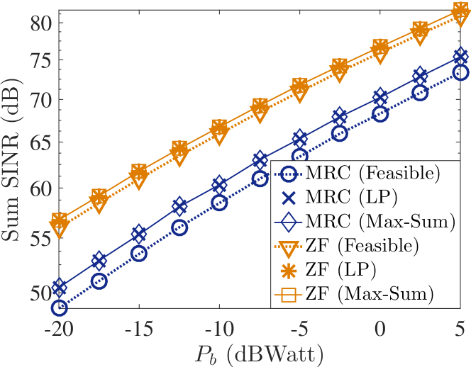
Figure 3: Sum of SINRs for the Max-Sum algorithm, LP, and orthogonal channel allocation.

Fig. 3 compares the sum of average SINR performance across all tags as a function of cores’ transmission power. As expected, for both ZF and MRC the proposed Max-Sum algorithm offers the same optimal performance with the relaxed LP technique and both outperform the channel allocation for which tags of the same cell use unique pairs $(m,c)\in\mathcal{M}_{\rm tr}\times\mathcal{C}$ (a feasible solution of problem (11)). The performance of the latter allocation is calculated across 1000 independent experiments. It can be remarked that the gap between ZF and MRC is $5$-$10$ dB, corroborating the intra-cell interference mitigation capabilities of ZF detector.

Fig. 4 shows how fast the proposed algorithm converges to the optimal $\mathbf{V}_{b}^{\star}$ and how many iterations are required until the termination criterion is reached at cores $2$ and $7$. For all cores the algorithm terminates after $5$-$10$ iterations on average, and for all cases the termination criterion of soft-estimates NMAE below $\epsilon$ was met. Also, the algorithm converges to the optimal solution within $2$-$3$ iteration at all cores. The above demonstrates the potential benefits of the proposed Max-Sum algorithm, since per iteration complexity is small and convergence is accomplished within few steps.

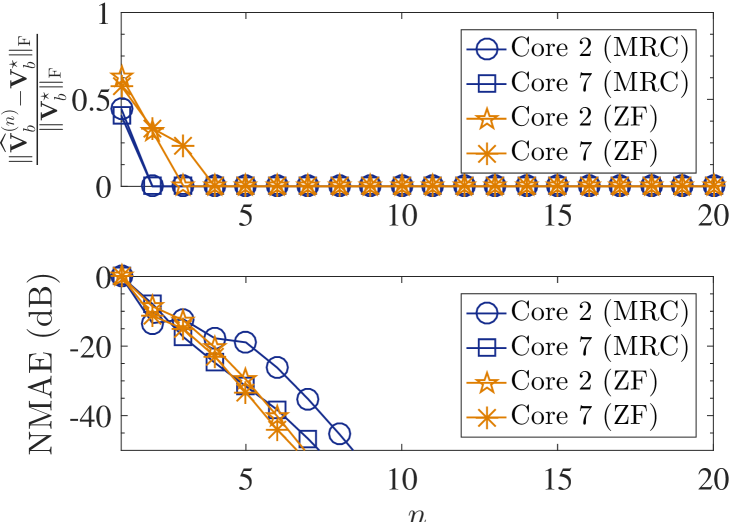
Figure 4: Convergence rate and NMAE of soft-estimates for the Max-Sum algorithm executed at cores $2$ and $7$.

Finally, one important question would be why one should use the proposed algorithm instead of classic LP to solve the studied optimization problem in (11). To this end, the proposed algorithm was compared with CVX convex optimization solver [13] in terms of average execution time across all cores. For the simulations, a computer with 64-bit operating system and Intel(R) Core(TM) i7-3540 and CPU at 3 GHz was used. The proposed algorithm was implemented with a custom MATLAB script, while the solution of LP relaxed problem was obtained by CVX solver. The average execution time, averaged across several transmit powers, for the proposed Max-Sun algorithm was $0.03$ sec and $0.033$ sec for ZF and MRC detectors, respectively, whereas, for the LP program with CVX solver required $0.424$ sec and $0.5$ for ZF and MRC detectors, respectively. This shows at least an order of magnitude improvement.

References

• [1] P. N. Alevizos, “Intelligent scatter radio, RF harvesting analysis, and resource allocation for ultra-low-power Internet-of-Things,” Ph.D. dissertation, Technical University of Crete, Chania, Greece, Dec. 2017.
• [2] G. Vannucci, A. Bletsas, and D. Leigh, “A software-defined radio system for backscatter sensor networks,” IEEE Trans. Wireless Commun., vol. 7, no. 6, pp. 2170–2179, Jun. 2008.
• [3] P. N. Alevizos, K. Tountas, and A. Bletsas, “Multistatic scatter radio sensor networks for extended coverage,” IEEE Trans. Wireless Commun., vol. 17, no. 7, pp. 4522–4535, Jul. 2018.
• [4] J. D. Griffin and G. D. Durgin, “Complete link budgets for backscatter-radio and RFID systems,” IEEE Antennas Propag. Mag., vol. 51, no. 2, pp. 11–25, Apr. 2009.
• [5] J. Kimionis, A. Bletsas, and J. N. Sahalos, “Bistatic backscatter radio for power-limited sensor networks,” in Proc. IEEE Global Commun. Conf. (Globecom), Atlanta, GA, Dec. 2013, pp. 353–358.
• [6] N. Fasarakis-Hilliard, P. N. Alevizos, and A. Bletsas, “Coherent detection and channel coding for bistatic scatter radio sensor networking,” IEEE Trans. Commun., vol. 63, pp. 1798–1810, May 2015.
• [7] P. N. Alevizos, A. Bletsas, and G. N. Karystinos, “Noncoherent short packet detection and decoding for scatter radio sensor networking,” IEEE Trans. Commun., vol. 65, no. 5, pp. 1–13, May 2017.
• [8] A. Goldsmith, Wireless Communications.   New York, NY, USA: Cambridge University Press, 2005.
• [9] A. Bletsas, A. G. Dimitriou, and J. N. Sahalos, “Improving backscatter radio tag efficiency,” IEEE Trans. Microw. Theory Techn., vol. 58, no. 6, pp. 1502–1509, Jun. 2010.
• [10] M. Bayati, C. Borgs, J. Chayes, and R. Zecchina, “On the exactness of the cavity method for weighted $b$-matchings on arbitrary graphs and its relation to linear programs,” Journal of Statistical Mechanics: Theory and Experiment, vol. 2008, no. 06, Jun. 2008.
• [11] T. Heskes, “On the uniqueness of loopy belief propagation fixed points,” Neural Comput., vol. 16, no. 11, pp. 2379–2413, Nov. 2004.
• [12] M. Bayati, C. Borgs, J. Chayes, and R. Zecchina, “Belief propagation for weighted $b$-matchings on arbitrary graphs and its relation to linear programs with integer solutions,” SIAM Journal on Discrete Mathematics, vol. 25, no. 2, pp. 989–1011, Jul. 2011.
• [13] M. Grant and S. Boyd, “CVX: Matlab software for disciplined convex programming, version 2.1,” http://cvxr.com/cvx, Mar. 2014.