The Peculiar Volatile Composition of CO-Dominated Comet C/2016 R2 (PanSTARRS)

Abstract

Comet C/2016 R2 (PanSTARRS) has a peculiar volatile composition, with CO being the dominant volatile as opposed to H${}_{2}$O and one of the largest N${}_{2}$/CO ratios ever observed in a comet. Using observations obtained with the Spitzer Space Telescope, NASA’s Infrared Telescope Facility, the 3.5-meter ARC telescope at Apache Point Observatory, the Discovery Channel Telescope at Lowell Observatory, and the Arizona Radio Observatory 10-m Submillimeter Telescope we quantified the abundances of 12 different species in the coma of R2 PanSTARRS: CO, CO${}_{2}$, H${}_{2}$O, CH${}_{4}$, C${}_{2}$H${}_{6}$, HCN, CH${}_{3}$OH, H${}_{2}$CO, OCS, C${}_{2}$H${}_{2}$, NH${}_{3}$, and N${}_{2}$. We confirm the high abundances of CO and N${}_{2}$ and heavy depletions of H${}_{2}$O, HCN, CH${}_{3}$OH, and H${}_{2}$CO compared to CO reported by previous studies. We provide the first measurements (or most sensitive measurements/constraints) on H${}_{2}$O, CO${}_{2}$, CH${}_{4}$, C${}_{2}$H${}_{6}$, OCS, C${}_{2}$H${}_{2}$, and NH${}_{3}$, all of which are depleted relative to CO by at least one to two orders of magnitude compared to values commonly observed in comets. The observed species also show strong enhancements relative to H${}_{2}$O, and even when compared to other species like CH${}_{4}$ or CH${}_{3}$OH most species show deviations from typical comets by at least a factor of two to three. The only mixing ratios found to be close to typical are CH${}_{3}$OH/CO${}_{2}$ and CH${}_{3}$OH/CH${}_{4}$. The CO${}_{2}$/CO ratio is within a factor of two of those observed for C/1995 O1 (Hale-Bopp) and C/2006 W3 (Christensen) at similar heliocentric distance, though it is at least an order of magnitude lower than many other comets observed with AKARI. While R2 PanSTARRS was located at a heliocentric distance of 2.8 AU at the time of our observations in January/February 2018, we argue, using sublimation models and comparison to other comets observed at similar heliocentric distance, that this alone cannot account for the peculiar observed composition of this comet and therefore must reflect its intrinsic composition. We discuss possible implications for this clear outlier in compositional studies of comets obtained to date, and encourage future dynamical and chemical modeling in order to better understand what the composition of R2 PanSTARRS tells us about the early Solar System.

1 Introduction

Comets are primitive, volatile-rich remnants from the formation of the Solar System, and for this reason their volatile composition is considered indicative of the physics and chemistry occurring in the protosolar disk during the planet formation stage. While there is diversity in compositions among the cometary population, comets consist primarily of H${}_{2}$O, followed by CO${}_{2}$ and CO at the 1-30% level, with trace species such as HCN, CH${}_{3}$OH, and C${}_{2}$H${}_{6}$ being present at the few percent level or less (MummaCharnley2011). The optical taxonomy of comets also shows diversity and evidence for modality (i.e. clumps of different compositional types), but in general optical cometary spectra are dominated by OH (and therefore H${}_{2}$O), with CN, C${}_{2}$, C${}_{3}$, CH, NH, and NH${}_{2}$ present at the percent level or less (e.g. AHearn1995; Cochran2012).
However, a few comets do not fit neatly into the established taxonomies. Comet 96P/Machholz shows an extremely atypical coma composition at optical wavelengths (though OH is still the dominant species), with a C${}_{2}$/CN ratio an order of magnitude higher than other comets (LanglandShulaSmith2007; Schleicher2008). Some comets, such as 29P/Schwassman-Wachmann 1, have observed CO/H${}_{2}$O ratios $>>$ 1 (Ootsubo2012), though this is often, at least partially, explained by its heliocentric distance being beyond the water ice line where water ice does not readily sublimate, meaning the observed coma composition is not necessarily indicative of the ice composition of the nucleus (WomackDistantReview2017).
Comet C/2016 R2 (PanSTARRS) was observed to have a peculiar optical spectrum when it was at a heliocentric distance of 3.1 AU, dominated by emissions from CO${}^{+}$ and N${}_{2}^{+}$ with a lack of emission from other species such as CN and C${}_{2}$ typically observed at these wavelengths (CochranMcKay2018). From these observations, it was derived that N${}_{2}$/CO $\sim$ 0.06, among the highest values observed in a comet. This result, coupled with the lack of many of the usual emissions observed in optical cometary spectra, suggested that this comet has a composition very different from any other comet observed to date. This was quickly communicated to the cometary science community for additional observations. Observations with the Arizona Radio Observatory 10-m Submillimeter Telescope (ARO SMT) confirmed a very high CO production rate and identified a low HCN abundance (WierzchosWomack2017; WierzchosWomack2018; deValBorro2018). Observations with the IRAM 30-meter telescope and the Nancay radio telescope provided a more complete picture of the volatile composition of R2 PanSTARRS, confirming the high CO abundance and anomalously low abundances of other volatiles such as HCN and H${}_{2}$O compared to CO (Biver2018). Additional high spectral resolution optical observations obtained with the UVES instrument on the VLT were reported by Opitom2019, confirming the findings of CochranMcKay2018 as well as providing new insights such as the first detection of [N I] emission in a cometary coma.
We present analysis of IR measurements obtained with the Spitzer Space Telescope and iSHELL on the NASA IRTF designed to quantify a suite of species observed in comets: H${}_{2}$O, CO${}_{2}$, CO, C${}_{2}$H${}_{6}$, CH${}_{3}$OH, CH${}_{4}$, H${}_{2}$CO, and OCS. We also present optical measurements used to study HCN (through CN emission), NH${}_{3}$ (through NH${}_{2}$ emission), N${}_{2}$ (through N${}_{2}^{+}$), C${}_{2}$H${}_{2}$ (through C${}_{2}$) and H${}_{2}$O (through OH and [O I]6300 Å emission), as well as new millimeter-wavelength observations of CO that are contemporaneous with our Spitzer observations. Section 2 presents our observations and Section 3 presents our analysis procedures and results. Section 4 discusses this truly peculiar comet in the context of current compositional taxonomies and possible implications for the physics and chemistry of the comet-forming region during the protoplanetary disk phase. Section 5 concludes the paper and encourages future work to better understand what R2 PanSTARRS reveals about the early Solar System.

2 Observations

We obtained observations in late January/February 2018 with several facilities, both space-borne and ground-based. These observations are detailed in Table 1.

Table 1: Observation Log

UT Date	R${}_{h}$ (AU)	$\dot{R_{h}}$ (km s${}^{-1}$)	$\Delta^{a}$ (AU)	$\dot{\Delta}^{a}$ (km s${}^{-1}$)	Solar Standard	Tell. Standard	Flux Standard
NASA IRTF iSHELL
January 30, 2018	2.81	-6.8	2.27	+17.2	-	HR 1165	HR 1165
ARO SMT
February 13, 2018	2.76	-6.0	2.41	+19.5	-	-	Chopper Wheel
Spitzer IRAC${}^{b}$
February 12, 2018	2.76	-6.0	2.26	-28.4	-	-	-
February 21, 2018	2.73	-5.5	2.11	-25.9	-	-	-
DCT LMI
February 21, 2018	2.73	-5.5	2.52	+20.3	-	-	HD 72526
							HD 37112
APO ARCES
January 30, 2018	2.81	-6.8	2.27	+17.2	Hyades 64	55 Persei	HR 1544

${}^{a}$Values for $\Delta$ and $\dot{\Delta}$ are the distance to the observer and velocity relative to the observer, respectively. Therefore for Spitzer observations these are relative to the Spitzer spacecraft, while for ground-based observations these are relative to Earth.
${}^{b}$Spitzer astronomical observation request (AOR) numbers: 65280768, 65281280, 65281024, 65281536

2.1 NASA IRTF iSHELL

We obtained Director’s Discretionary Time to observe R2 PanSTARRS with the powerful iSHELL IR spectrograph on the NASA IRTF on Maunakea, HI on UT January 29 and 30, 2018. While poor weather precluded obtaining useful data on January 29, we obtained high quality spectra on January 30. The iSHELL detector is a 2048 $\times$ 2048 pixel Hawaii H2RG array with sensitivity over a wavelength range of $\sim$ 1-5 $\mu$m. As a cross-dispersed instrument, iSHELL measures signal in many ($>$10) consecutive echelle orders simultaneously with complete (for $\lambda\leq 4$ $\mu$m) or nearly complete (for $\lambda>4$ $\mu$m) spectral coverage, a significant improvement over the previous IRTF high-resolution facility spectrograph, CSHELL (Tokunaga1990). More details on iSHELL can be found in Rayner2012; Rayner2016.
For our observations of R2 PanSTARRS, we used the 0.75″ wide slit, which provides a spectral resolution of R $\equiv$ $\frac{\lambda}{\delta\lambda}$ $\sim$ 38,000 for a uniform monochromatic source. We also observed an early type IR standard star with the 4″ wide slit to serve as a flux calibrator and a telluric standard (see Section 3.1). This slit provides lower spectral resolution (R $\sim$ 20,000), but minimizes slit losses and therefore systematic errors in flux calibration. Both the comet and standard star were observed using the classic ABBA nodding sequence, with a 7.5″ telescope nod (half the slit length) along the slit between the A and B positions, located equidistant to either side of the slit midpoint. We employed two grating settings: M2 and Lp1. M2 covers a wavelength range of $\sim$ 4.52 - 5.25 $\mu$m, encompassing spectral lines of CO, H${}_{2}$O, and OCS. Lp1 covers the wavelength range $\sim$ 3.28-3.65 $\mu$m and targets emission from CH${}_{4}$, C${}_{2}$H${}_{6}$, CH${}_{3}$OH, H${}_{2}$CO, and OH prompt emission (a well established proxy for H${}_{2}$O production in comets (Bonev2006)). Our comet observations resulted in 29.2 minutes on source in M2 and 59.8 minutes on source in Lp1. We obtained flats and darks at the end of each observing sequence for each grating setting.
Guiding was achieved through filter imaging with the slit-viewer camera, performed in specific wavelength bands independent of the wavelength regime used to obtain spectra. The slitviewer allows active guiding on sufficiently bright targets while obtaining spectra. Short time-scale guiding is achieved through a boresight guiding technique, which utilizes “spillover” flux that falls outside the slit to keep the optocenter on the slit. However, while easily visible in the guider using a broadband J filter, R2 PanSTARRS was not bright enough for active guiding. We instead performed offset guiding using a reference (guide) star in the slitviewer field of view (FOV). Owing to the small non-sidereal rates of R2 PanSTARRS, this worked very well; we verified that the comet’s position with respect to the slit remained very stable over the course of our observations, with minimal adjustments needed to keep it in the slit. More details relevant to cometary observations using iSHELL are presented in DiSanti2017.

2.2 Arizona Radio Observatory Sub-millimeter Telescope (SMT)

Observations of the CO(2-1) line at 230.53799 GHz were performed with the Arizona Radio Observatory 10-m Submillimeter Telescope on 2018 February 13 at 5:16 UT using the 1.3 mm dual polarization receiver with ALMA Band 6 sideband-separating mixers. The observations began 11 hours after the first Spitzer epoch. Data acquisition was done in beam-switching mode with a +2′ throw in azimuth and standard 6 minute scans were acquired. System temperatures had peak values of 390K, but on average remained under 340K. The chopper wheel method was used to determine the temperature scale for the SMT receiver systems with a beam efficiency of $\eta$ = 0.74. The backend configuration that provided the best velocity resolution (0.325 km s${}^{-1}$ per channel) consisted of a 2048 channel 250 kHz/channel filterbank in parallel mode. Accuracy of the pointing and tracking was checked against the JPL Horizon’s ephemeris position and was found to be better than $<$ 1″ rms. Due to high winds, only 12 scans were obtained but the CO line was strong enough to be seen in single scans.

2.3 Spitzer IRAC

We obtained Director’s Discretionary Time to observe R2 PanSTARRS with Spitzer IRAC on 2018 February 12 at 18:22 UT and 2018 February 21 at 01:03 UT in order to measure the CO${}_{2}$ production rate. As Spitzer is well into its post-cryogenic mission, IRAC presently observes in two pass bands: one centered at 3.6 $\mu$m and the other at 4.5 $\mu$m. Both filters have broad wavelength coverage, with bandwidths of 0.8 and 1.0 $\mu$m, respectively. The 4.5 $\mu$m band has been used extensively in the past for measuring CO${}_{2}$ production rates in comets, as this bandpass includes the $\nu_{3}$ band of CO${}_{2}$ at 4.26 $\mu$m (e.g. Reach2013; McKay2016). It also contains the $\nu$(1-0) band of CO at 4.7 $\mu$m, but in many comets in the AKARI survey (Ootsubo2012), the CO${}_{2}$ feature was at least 10 times brighter than the CO feature, and so CO${}_{2}$ is typically assumed to be the dominant gas emission feature in the IRAC 4.5 $\mu$m band. This is due to the fluorescence efficiency of CO${}_{2}$ being approximately an order of magnitude larger than that for CO coupled with the fact that the CO${}_{2}$ abundance in comets is often equal to or greater than the CO abundance. There are examples, however, such as C/2006 W3 (Christensen) and 29P/Schwassman-Wachmann 1, where CO emission contributes significantly to the 4.5 $\mu$m band flux (Ootsubo2012; Reach2013). The high CO production rate found for R2 PanSTARRS (WierzchosWomack2018; deValBorro2018; Biver2018) means CO emission may not be negligible in the Spitzer imaging, and may in fact dominate signal in the 4.5 $\mu$m channel. We discuss how we account for the CO contribution in the Spitzer imaging in Section 3.3.
We supply details of our observations in Table 1. The IRAC array is a 256 x 256 pixel InSb array, covering a 5.2′ x 5.2′ FOV with a spatial scale of 1.2″/pixel, which for our observations corresponds to a projected FOV of $\sim$500,000 km and a spatial scale of $\sim$1900 km/pixel. We employed a 9-position random dither pattern. Each bandpass is observed with independent arrays, such that when one array is observing the comet, the other is on an adjacent field. The sequence takes about 12 minutes to execute. For each epoch we performed observations of the comet field several days after each cometary observation in order to image the field without the comet in it. These images are termed “shadow observations” and provide a measurement of the background to be subtracted from the cometary images. Our observations were obtained in high dynamic range (HDR) mode, which entailed obtaining exposures with both short (1.2 s) and long (30 s) exposure times in order to avoid saturation of the inner coma, while still keeping high signal-to-noise ratio (SNR) in the fainter outer coma. Observing in HDR mode also helps protect against saturation due to bright field stars. For these observations no pixels were saturated; therefore to optimize SNR we analyzed the longest exposure time images.

2.4 Discovery Channel Telescope-Large Monolithic Imager, (LMI)

We observed R2 PanSTARRS with the Large Monolithic Imager (LMI) on the 4.3-m Discovery Channel Telescope (DCT) at Lowell Observatory from 2:51–4:13 UT on February 21, 2018. The observations were a Target of Opportunity (ToO) request that interrupted normal observations and began within 2 hours of the Spitzer observations in order to provide a near-simultaneous constraint on the water production of R2 PanSTARRS. DCT ToO requests are limited to 2 hr, which allowed us sufficient time to focus the instrument, observe high and low airmass standard stars (listed in Table 1), and obtain $\sim$83 minutes on R2 PanSTARRS. Conditions were photometric with seeing $\sim$1.2″. The comet was $\sim$33${}^{\circ}$ from a 26% illuminated moon, although no stray light attributable to the moon was evident in any of our images. The comet’s airmass ranged from 1.06 to 1.23.

LMI has a 12.3′$\times$12.3′ field of view and $6.1\mathrm{K}{\times}6.1\mathrm{K}$ e2v CCD. On-chip $3{\times}3$ binning resulted in a pixel scale of 0.36″/pixel. We obtained images using a standard broadband SDSS-$r^{\prime}$ filter and narrowband ion (CO${}^{+}$ central wavelength/bandpass width=4266 Å/64 Å), gas (OH 3090/62, CN 3870/62), and dust continuum (UC 3448/84, BC 4450/67) filters that are all part of the comet Hale-Bopp set (Farnham2000). Single frames were acquired at the start and end of the sequence in the two filters with the highest signal-to-noise, $r^{\prime}$ (30 s) and CO${}^{+}$ (300 s). In between, sets of exposures were acquired in OH (3 exposures each of 600 s), UC (3$\times$300 s), and BC (2$\times$120 s), with the sets proceeding from shortest to longest wavelength in order to minimize the effects of atmospheric extinction as the airmass increased. A single CN exposure (180 s) was also acquired at the end of the sequence. The telescope followed the comet’s ephemeris rate for all comet images.

2.5 Apache Point Observatory-ARCES

We obtained Director’s Discretionary Time to observe R2 PanSTARRS with the ARCES instrument on the Astrophysical Research Consortium (ARC) 3.5-meter telescope at Apache Point Observatory (APO) in Sunspot, NM on UT January 30, 2018, just hours before the iSHELL observations. ARCES provides a spectral resolving power of R = 31,500 and a spectral range of 3500-10,000 Å with no interorder gaps. More specifics for this instrument are discussed elsewhere (Wang2003).
Observational details are described in Table 1. For all observations we centered the 1.6″$\times$3.2″ slit on the optocenter of the comet. We obtained six spectra of 1800 s each over the course of the night. These spectra were averaged after extraction and calibration to increase SNR. We obtained an ephemeris generated from JPL Horizons for non-sidereal tracking of the optocenter. For short time-scale guiding, the guiding software employs a boresight technique to keep the optocenter centered in the slit. We observed a G2V star in order to remove the underlying solar continuum and Fraunhofer absorption lines, a fast rotating (vsin(i) $>$ 150 km s${}^{-1}$) B star to account for telluric features, and spectra of a flux standard to establish absolute intensities of cometary emission lines. The calibration stars used are given in Table 1. We obtained spectra of a quartz lamp for flat fielding and acquired spectra of a ThAr lamp for wavelength calibration.

3 Data Analysis and Results

3.1 IRTF-iSHELL

Figure 1 shows raw spectral-spatial difference frames (total A-beam minus B-beam exposures) of R2 PanSTARRS for our M2 (left) and Lp1 (upper right) observing sequences. We applied our general methodology for processing IR spectra (e.g. DelloRusso2006; Villanueva2011; DiSanti2014). New techniques specific to iSHELL are described in detail in DiSanti2017 (see also Roth2018). We provide a brief summary of our reduction procedures below.
Processing of each iSHELL order produces a “rectified” spectral-spatial frame, meaning each column pertains to a unique wavelength and each row to a unique spatial location along the slit. An example is shown in Figure 1 for the region of Lp1 order 157 containing the cometary R0 and R1 lines of CH${}_{4}$ (panel (e), bottom-right). Such rectified orders consist of three parts: the bottom and top thirds show comet signal obtained from A-beam and B-beam observations, respectively (in black), and the middle third shows the combined signal [(A+B)/2] (in white). Spectral extracts for the standard star and comet are obtained by summing signal over a range of rows in the central (combined-beam) portion of their rectified frames.

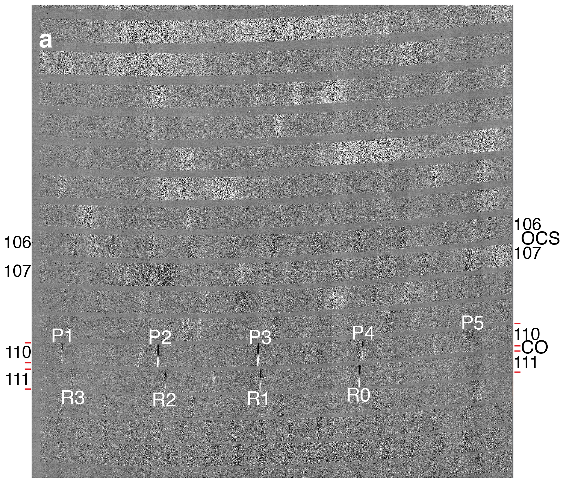
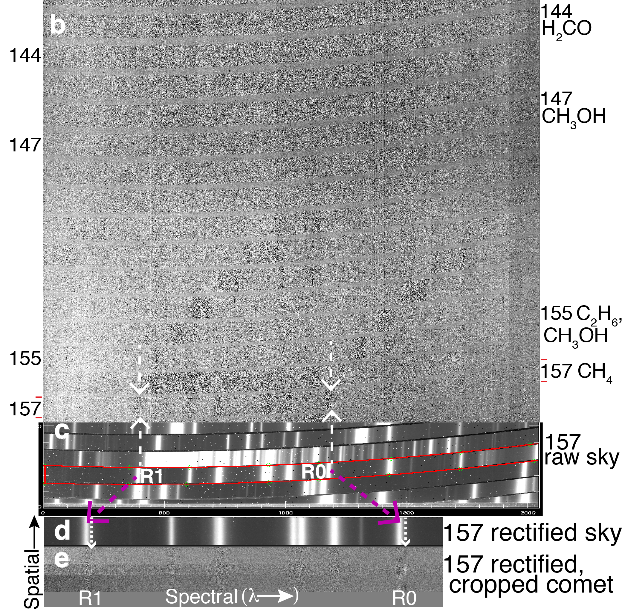
Figure 1: Raw spectral-spatial stacks (A-B difference frames) of R2 PanSTARRS obtained with iSHELL in the (a) M2 and (b) Lp1 settings on UT 30 January 2018, with echelle orders relevant to our study indicated (106, 107, 110 and 111 for M2; 144, 147, 155, and 157 for Lp1), and with molecules targeted in each order listed at right. CO emission lines (labeled with their rotational designations) are clearly seen in M2 orders 110 and 111, with the A-beam signal in white and the B-beam signal in black. Conversely, no emission lines are readily apparent in the Lp1 stack. (c) Portion of the corresponding Lp1 raw sky frame that includes order 157, outlined in red and spectrally aligned with the raw comet stack. Expected positions of the cometary CH${}_{4}$ lines are depicted by vertical white dashed arrows immediately to the right/red of the corresponding sky emission lines, in accordance with the geocentric velocity of R2 PanSTARRS ($\dot{\Delta}=+17.2$ km s${}^{-1}$; Table 1). (d) Sky emission centered around the CH${}_{4}$ lines in order 157, after being rectified as explained in the text. (e) Corresponding rectified order for R2 PanSTARRS, again with the cometary CH${}_{4}$ lines Doppler-shifted from their telluric counterparts. The combined comet signal (in white) is shown as the middle portion and, above and below this (in black) individual B- and A-beams, respectively. For spectral extracts from the CO and CH${}_{4}$ orders, see Fig. 2.

To achieve absolute flux calibration, and to determine the column burdens of absorbing species in the terrestrial atmosphere, we fit a synthetic atmospheric transmittance model to the standard star spectrum for each processed order. We applied this optimized atmospheric transmittance model (calculated at the airmass of R2 PanSTARRS), convolved it to the spectral resolution of the cometary observations and scaled it to the cometary continuum level (the continuum is virtually absent for our observations of R2 PanSTARRS). Subtracting the scaled model yields the net observed cometary emission spectrum, still multiplied by monochromatic atmospheric transmittance at the Doppler-shifted frequency of each cometary line. Correcting for transmittance and incorporating flux calibration factors from our standard star spectra allows establishing line fluxes incident at the top of the terrestrial atmosphere. Fully calibrated spectral extracts for R2 PanSTARRS showing emission lines of CO and CH${}_{4}$ are shown in Figure 2. All other species searched for were not detected.

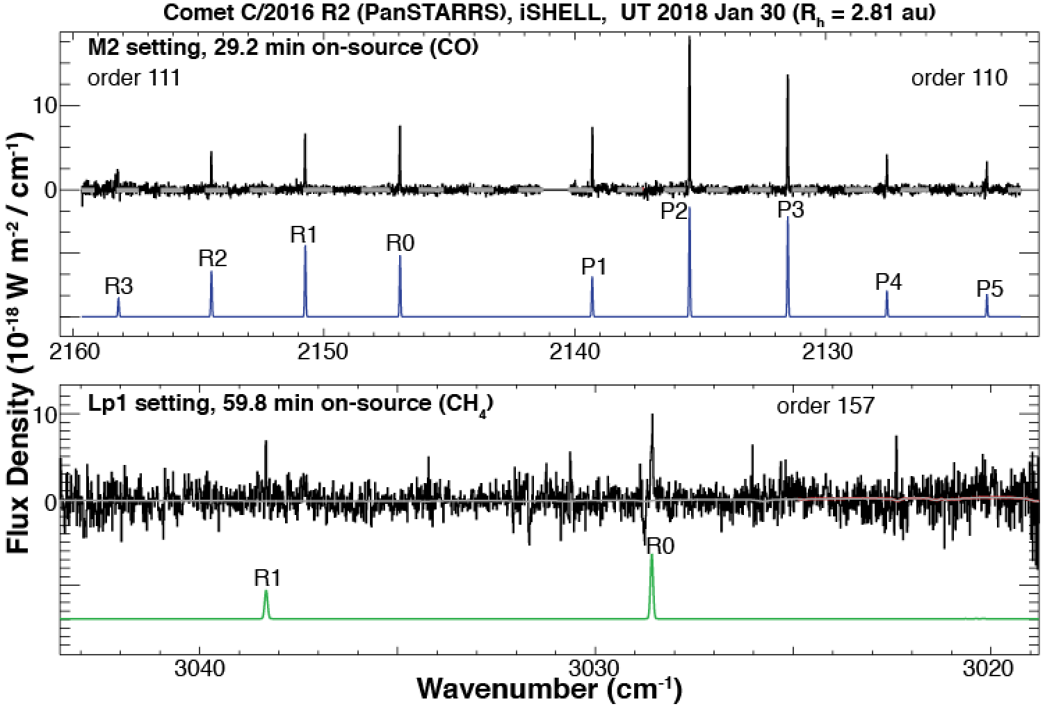
Figure 2: Spectra and corresponding fluorescence model fits to observed CO (top) and CH${}_{4}$ (bottom) emission in R2 PanSTARRS obtained with iSHELL. Each spectrum represents the signal summed over 15 rows (2.25”) centered on the peak emission, and each line is labeled with its rotational identification. We detected nine CO lines spanning two echelle orders, and two CH${}_{4}$ lines within a single order.

We establish molecular column densities (or upper limits) by dividing these transmittance-corrected line fluxes by appropriate line-specific fluorescence g-factors, the values of which depend on rotational temperature ($T_{rot}$). For our study of R2 PanSTARRS with iSHELL, only CO presented enough lines with high signal-to-noise that spanned a sufficient range of rotational energy to obtain a measure of $T_{rot}$. Because the solar spectrum contains CO absorption lines, an accurate treatment required using “reduced” CO g-factors that incorporate the Swings effect for the heliocentric velocity of the comet at the time of our observations (-6.8 km s${}^{-1}$; see Table 1). Our analysis of CO provided a best-fit value $T_{rot}$ = 13$\pm$2 K. We assume this temperature also applies to other species, as observations of brighter comets in which $T_{rot}$ was measured for multiple species demonstrate that this is generally a valid assumption (e.g. DelloRusso2011; Mumma2011; Gibb2012; DiSanti2014).
We obtained molecular production rates as follows. We extracted a “nucleus-centered” spectrum by summing signal over 15 rows ($\sim$ 2.5″) centered on the row containing the peak emission line intensity. Application of Swings-corrected g-factors and geometric parameters (R${}_{h}$, $\Delta$, beam size at the comet) to transmittance-corrected line fluxes provides the nucleus-centered production rate, Q${}_{nc}$. However, owing primarily to seeing, Q${}_{nc}$ invariably underestimates the actual “total” (or “global”) production rate, Q${}_{tot}$. To obtain Q${}_{tot}$ we multiplied each Q${}_{nc}$ by an appropriate growth factor (GF), determined through the well-documented “Q-curve” method for analyzing spatial profiles of emissions (DelloRusso1998). For each spatial step, a “symmetrized” Q-curve was produced by averaging signal at equal but diametrically opposed distances from the nucleus. For our observations, only CO and CH${}_{4}$ were detected. Each showed bright enough emissions to allow a reliable Q-curve analysis to be performed.
We present spatial profiles and symmetrized Q-curves for CO and CH${}_{4}$ in Fig. 3. For each Q-curve, GF is depicted graphically as the level of the upper horizontal line (representing Q${}_{tot}$) divided by that of the corresponding lower horizontal line (representing Q${}_{nc}$). We refer to the region of the coma over which Q${}_{tot}$ is measured as the “terminal region.”

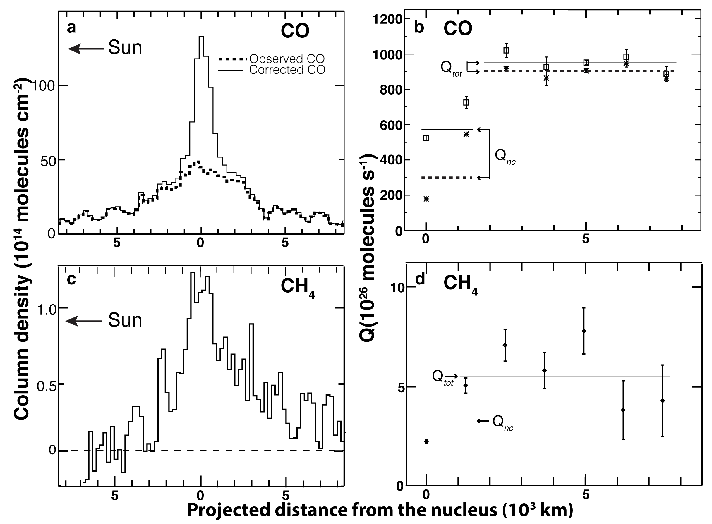
Figure 3: Spatial profiles (left) and symmetrized Q-curves (right) from our iSHELL observations of R2 PanSTARRS, representing the sum of 9 CO lines (top) and the sum of 2 CH${}_{4}$ lines (bottom). For the spatial profiles, the sunward-facing hemisphere is to the left as indicated. For CO (panels a and b), dashed traces/lines represent observed emission while solid traces/lines represent emission after correcting line-by-line for optical depth in the solar pump, following the methodology of DiSanti2001. In all cases, GF is given by the ratio of total Q (Q${}_{tot}$, upper horizontal line) to nucleus-centered Q (Q${}_{nc}$, corresponding lower horizontal line). The GF for CO prior to correcting for optical depth (2.93$\pm$0.04) is much larger than that measured for (optically thin) CH${}_{4}$ (1.70$\pm$0.19). However, the opacity-corrected CO Q-curve has a much lower GF = 1.67$\pm$0.04, consistent with that for CH${}_{4}$. We note that for CO our formalism for correcting optical depth increases Q${}_{nc}$ by 91%, but increases Q${}_{tot}$ by only 5.6% (well within 1-$\sigma$ uncertainty; see Table LABEL:Qrates). This suggests that our approach for modeling optical depth, coupled with the Q-curve formalism, provides robust production rates for these two species in R2 PanSTARRS.

Comparison of the profiles in Fig. 3 reveals a relatively broad (and in particular a “flat-topped”) spatial distribution for the observed CO emission. This is demonstrated by its much larger GF compared to CH${}_{4}$, and also that leveling its Q-curve required beginning two steps from the nucleus instead of one step, as was used for CH${}_{4}$. This could indicate extended release of CO (e.g., from grains) in the inner coma, and/or optical depth in the CO lines (particularly along lines-of-sight passing close to the nucleus). The high CO production rates reported from millimeter observations of R2 PanSTARRS with IRAM (Biver2018) and SMT (WierzchosWomack2018), as well as from our iSHELL observations (see Table 3) suggest the IR lines of CO are affected by optical depth.
Several previous CO-rich comets revealed optically thick emissions that in all cases were most pronounced for lines-of-sight passing through the innermost coma. For observations of C/1995 O1 (Hale-Bopp) and C/1996 B2 (Hyakutake) with CSHELL at the IRTF, observed column densities and Q-curves were corrected for opacity in the solar pump assuming uniform gas outflow at constant speed (DiSanti2001; DiSanti2003). Observations of C/2006 W3 (Christensen) with CRIRES at the ESO/VLT (Bonev2017) at a similar observing geometry to our observations of R2 PanSTARRS also revealed optically thick CO for a production rate only slightly lower than has been reported for R2 PanSTARRS.  Bonev2017 developed a formalism for addressing optical depth effects in CO emission based on a curve-of-growth analysis, demonstrating through their Q-curve analysis that the effects of optical depth on retrieved production rates can be quantified (and thus corrected for).
Provided that signal in the terminal region (i.e., the ends of the slit farthest from the comet optocenter) approximates optically thin conditions, the Q-curve will level out, as was observed for these three previously observed CO-rich comets, and as we also observed for R2 PanSTARRS (Fig. 3). Although in this case for CO the central region is optically thick, the GF still allows establishing a reliable approximation of the actual Q${}_{tot}$, but with the GF for CO being significantly larger than the corresponding value for the optically thin CH${}_{4}$ emission in R2 PanSTARRS (see Fig. 3). For all these comets (including R2 PanSTARRS), Q${}_{tot}$(CO) as retrieved from optically thin and optically thick treatments are in formal agreement (i.e., they agree to within their respective 1-$\sigma$ uncertainties); see Fig. A4 of DiSanti2001, Fig. 4 of DiSanti2003, and Fig. 4 of Bonev2017. We demonstrate this by applying the methodology detailed in the Appendix of DiSanti2001 to the observed CO emission in R2 PanSTARRS. The presence of optically thick CO emission in R2 PanSTARRS is supported by the much larger GF for the observed CO profile (2.93 $\pm$ 0.04) versus that for (optically thin) CH${}_{4}$ (1.70 $\pm$ 0.19), a discrepancy that is resolved by correcting for optical depth in the CO lines (resulting in 1.67 $\pm$ 0.04, see Fig. 3b). Therefore we conclude that our Q-curve analysis for CO mitigates the effects of optical depth on our measured CO production rate. It also reinforces our decision to apply its “corrected” GF (1.7) to obtain a realistic upper limit for co-measured OCS, and similarly to constrain Q${}_{tot}$ using the (identical within 1-$\sigma$ uncertainty) GF from CH${}_{4}$ for co-measured, undetected species included in the Lp1 setting (C${}_{2}$H${}_{6}$, CH${}_{3}$OH, and H${}_{2}$CO). Derived production rates and mixing ratios are shown in Table LABEL:Qrates.
Our spatial profiles also permit testing for asymmetric gas outflow in the coma. This is very pronounced for CH${}_{4}$ (Fig. 3c), indicating a large enhancement in the anti-sunward facing hemisphere, particularly considering the relatively small solar phase angle of R2 PanSTARRS at the time of our observations ($\sim$ 19${}^{\circ}$) and thus the potential high degree of projection onto the sky plane. The column density of CH${}_{4}$ averaged between $\sim$ 2,000 and 8,000 km from the nucleus (projected on the sky) is a factor of 2.65$\pm$0.55 larger in the anti-sunward direction compared to the solar direction, while the CO profile is much more symmetric, its corresponding ratio being only 1.03$\pm$0.02.
It is possible that the asymmetry observed for CH${}_{4}$ is associated with rotation of the nucleus. However, for the measured gas speed v${}_{exp}$ of 0.52 km s${}^{-1}$ (from our SMT observations, see Section 3.2) the time required to exit the iSHELL terminal region (extending to 4.9” from the nucleus) is approximately 4.3 hours, longer than the clock times encompassed by our M2 and Lp1 sequences (obtained consecutively and together spanning 2.65 hours of elapsed clock time). This suggests that gas in the iSHELL slit was not replenished (at least significantly) between M2 and Lp1 observations, and thus the large differences in the degrees of asymmetry observed for CO and CH${}_{4}$ cannot be explained by temporally variable outgassing. Nonetheless, these results indicate that the abundance ratio CH${}_{4}$/CO was higher in the anti-sunward-facing hemisphere than in the sunward-facing hemisphere by a factor of $\sim$ 2.5 and therefore, assuming little to no replenishment of coma gas between M2 and Lp1 sequences, this implies a significantly higher CH${}_{4}$/CO abundance ratio in the anti-sunward direction at the time of our iSHELL observations.

3.2 ARO-SMT

Figure 4 shows the spectrum resulting from coadding all 12 scans on UT February 13. We calculated the column density assuming optically thin gas (appropriate for the relatively large beam diameter of 32$\arcsec$) with T${}_{rot}$=23K (Biver2018, see Section LABEL:sec:discuss for discussion of difference with iSHELL), and we calculated the production rate assuming a simple symmetric outflow expansion model with V${}_{exp}$=0.52 km s${}^{-1}$ consistent with our spectra and other detailed modeling of the spectral line profiles (WierzchosWomack2018; Biver2018). We adopt this expansion velocity for all analysis in this work. The CO production rate is (5.5 $\pm$ 0.89) $\times$ 10${}^{28}$ mol/s (see Table LABEL:Qrates).

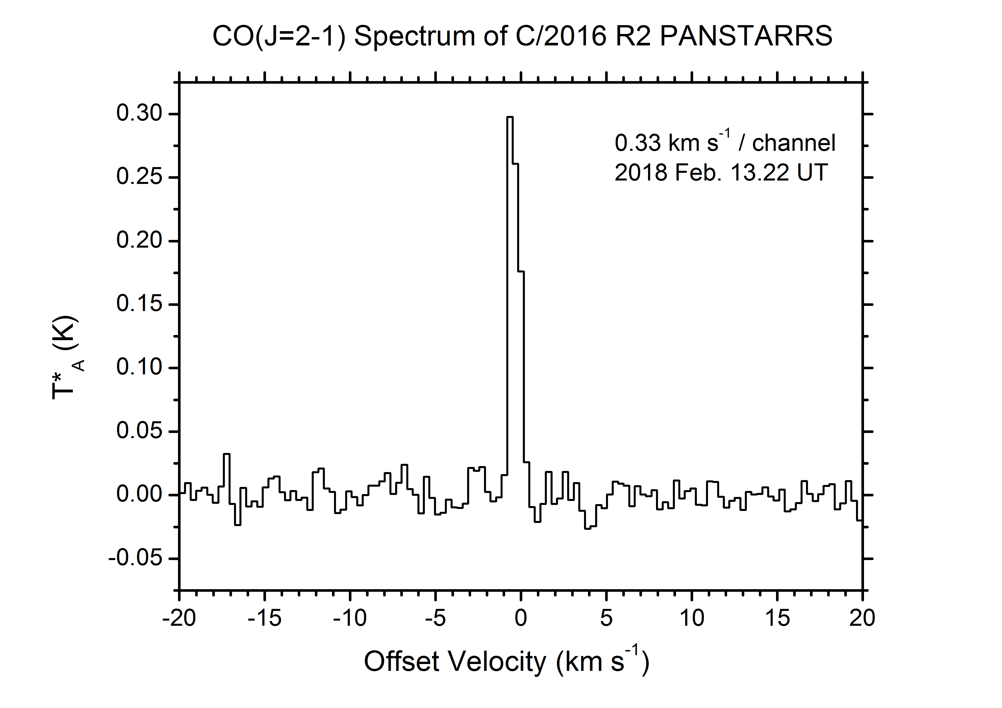
Figure 4: Spectrum of CO J=2-1 emission from comet C/2016 R2 obtained with the ARO SMT 10-m telescope on Feb. 13.22 2018 UT.

3.3 Spitzer IRAC

We combined all images of the same exposure time using the MOPEX software (Makovoz2005). This process creates a mosaic in the rest frame of the comet from the individual images, averaging overlapping data together, but ignoring cosmic rays and bad pixels. Two mosaics are created: one for the comet data, the other for the shadow (background) data. We subtracted the shadow mosaic from the comet mosaic to remove the background. This includes zodiacal light and celestial sources. While this removes background stars and most of the sky background, it may not completely remove the sky background (for instance, zodiacal light for a given RA and Declination varies with time). We used the sky value from the adjacent image of blank sky to remove any residual background that remained after shadow subtraction. The resulting images are shown in the first two columns of Fig. 5.

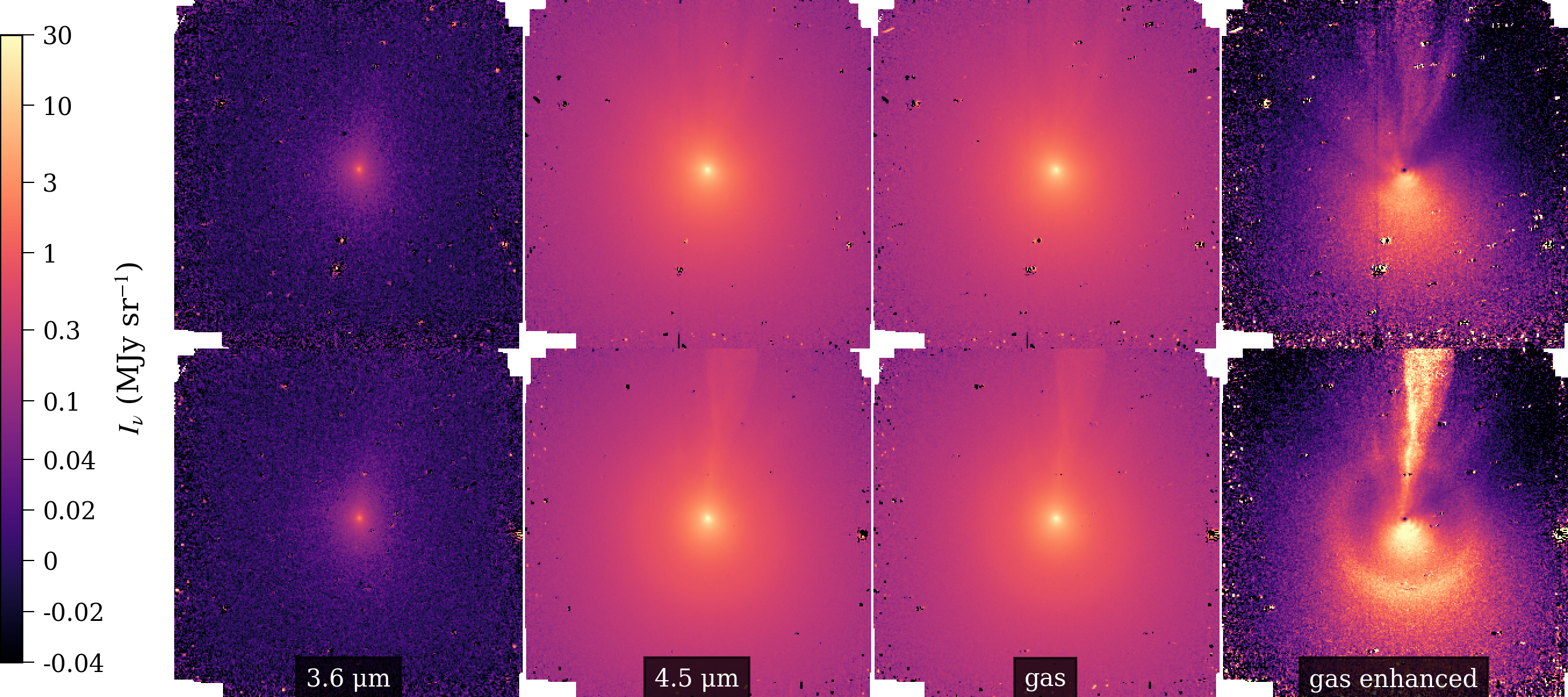
Figure 5: Shadow-subtracted images of C/2016 R2 (PanSTARRS) obtained with Spitzer IRAC at 3.6 $\mu$m (leftmost column) and 4.5 $\mu$m (left middle column), as well as the dust-subtracted images (right middle column) on UT February 12, 2018 (top row) and UT February 21, 2018 (bottom row). These images are for the longer exposure time (30 s) in our HDR mode observations. The solar direction is downward in all images. The spherical coma geometry observed in the 4.5 $\mu$m channel, as well as the large flux ratio between the two filters, is indicative of a large gas contribution to the observed flux, due to CO${}_{2}$ and CO. The last column shows the dust-subtracted images normalized by a $\rho^{-1}$ surface brightness distribution, where $\rho$ is the projected distance to the peak brightness, which enhances coma asymmetries. There is clear evidence for a strong ion tail, which we attribute to CO${}^{+}$ (see Discussion). There is also a clear spiral structure in the inner-most coma indicative of a rotating jet and a large circular arc that is present on February 21 but not February 12, possibly indicative of an impulsive outgassing event in between the two observation epochs. On both dates there is broad sunward enhancement indicative of preferential outgassing from the sunward hemisphere, which is consistent with results from CO spectral line profiles and spatial mapping measured at millimeter wavelengths (WierzchosWomack2018; Biver2018). A more detailed analysis of the coma morphology is beyond the scope of this paper and will be deferred to a future publication.

After the mosaic images were created and the sky background was subtracted, we removed the dust contribution from the 4.5 $\mu$m band flux, isolating the gas emission. As the level of dust contamination is minimal as inferred from the 3.6 $\mu$m image being much fainter than the 4.5 $\mu$m image (see Fig. 5), we simply applied a scaling factor of 0.9 to the 3.6 $\mu$m image and subtracted it from the 4.5 $\mu$m image to remove the dust contribution from the 4.5 $\mu$m image. The scale factor of 0.9 was derived from a model for cometary dust accounting for the expected contributions of reflected light and thermal emission at the heliocentric distance of R2 PanSTARRS, based on the empirical coma dust model of Kelley2016 and the dust color of comet 67P/Churyumov-Gerasimenko at 2.8 au (Snodgrass2017). The resulting dust-subtracted images are shown in the right center column of Fig. 5. The right-most column of Fig. 5 shows the dust-subtracted images normalized by a $\rho^{-1}$ surface brightness distribution, where $\rho$ is the projected distance to the peak brightness, which enhances coma asymmetries. The enhanced images show strong spiral structures as well as an ion tail that we attribute to CO${}^{+}$ (see Section LABEL:sec:discuss). A more detailed analysis of the coma morphology is beyond the scope of this paper.
As mentioned in Section 2.3, CO likely contributes significant flux to the Spitzer 4.5 $\mu$m channel, especially considering the large CO production rates measured for R2 PanSTARRS at millimeter-wavelengths (WierzchosWomack2018; Biver2018) and in the IR with iSHELL (Fig. 3b). CO${}_{2}$ is also observed with strong emission at this wavelength in many comets (Ootsubo2012), with few other likely contributors (see Section LABEL:sec:discuss for a discussion of other possible contaminating species). Therefore, we assume that the gas emission at 4.5 $\mu$m predominantly arises from CO and CO${}_{2}$, and separate their contributions with a three-step process: 1) we initially assume that 100% of the gas emission flux comes from CO molecules and derive a CO production rate, 2) subtract the contemporaneous ground-based measured CO production rate taking care to match the projected photometric aperture used for the Spitzer observations, which leaves a residual amount, and 3) then re-characterize this residual as a CO${}_{2}$ production rate.
From the dust-subtracted image of gas emission, we measured the flux for apertures ranging from 10-100 pixels (12-120″) in radius. We converted the broadband photometry to CO line fluxes in photons following the IRAC data handbook (Laine2015). The line fluxes were then used to calculate the total number of CO molecules inside the photometric aperture ($N_{CO,100\%}$) using

$$N_{CO,100\%}=4\pi\Delta^{2}F\frac{R_{h}^{2}}{g_{CO}}$$ (1)

where $\Delta$ is the Spitzer-comet distance, $F$ is the observed photon flux, $R_{h}$ is the heliocentric distance of the comet, and $g_{CO}$ is the g-factor for excitation of the CO 1$\rightarrow$0 fundamental vibrational band, which is 2.5 $\times$ 10${}^{-4}$ photons s${}^{-1}$ (Debout2016). Then the production rate $Q_{CO,100\%}$, is given by

$$Q_{CO,100\%}=\frac{2v}{\pi\rho}N_{CO,100\%}$$ (2)

where $N_{CO,100\%}$ is the total number of CO molecules in the photometric aperture, $v$ is the expansion velocity, and $\rho$ is the projected radius of the photometric aperture. We assume an expansion velocity of the coma of 0.52 km/s consistent with CO line widths from our SMT observations (see Section 3.2) and with expansion velocities reported for R2 PanSTARRS by WierzchosWomack2018 and Biver2018. This approach assumes a negligible effect of photodissociation on the spatial profile in the photometric aperture, which is justified as our photometric apertures are $<$ 10% of both the CO${}_{2}$ and CO photodissociation scale lengths. We calculated production rates for a variety of aperture sizes to quantify any trends in derived production rates with aperture size. Since we found the deviations between derived production rates for different aperture sizes to be minimal ($<$ 5%), for the rest of this paper we quote production rates derived using a photometric aperture that matches the projected distance at the comet of the ARO SMT observation beam (see Section 2.2). This is a 14-pixel radius on UT February 12 and a 15-pixel radius on UT February 21. This choice minimizes systematic errors when subtracting the expected CO flux from the Spitzer images (see below).
If we assume that all the gas flux in the Spitzer 4.5 $\mu$m image is due to CO and calculate its corresponding production rate using equations (1) and (2), we find Q${}_{CO,100\%}$ $\sim$ 1.6 $\times$ 10${}^{29}$ mol/s, higher than values derived from ground-based CO observations (WierzchosWomack2018; Biver2018; deValBorro2018, and this work). Therefore we conclude that CO is probably not the sole contributor to the observed flux. However, it is a major contributor and accounting for it does have a strong influence on the derived CO${}_{2}$ production rate. While CO contributes significantly to the observed Spitzer fluxes, the excess we attribute to CO${}_{2}$ is still $>$ 50% of the observed flux, so the detection of CO${}_{2}$ is robust.
To calculate $Q_{CO_{2}}$ and account for the CO contribution to the Spitzer 4.5 $\mu$m images, we employ our contemporaneous observations of CO at mm-wavelengths obtained with the ARO SMT (section 2.2). We favor using the contemporaneous SMT results over the IRTF CO measurements from several weeks earlier for subtraction of the CO contribution from the Spitzer imaging in order to minimize effects due to possible comet variability. Moreover, the production rates from SMT and Spitzer data were obtained using the same sized photometric aperture, whereas the iSHELL observations cover a much smaller projected region of the coma, making it more sensitive to short-time scale changes in gas production such as rotational variation. This approach minimizes systematic uncertainties introduced by possible variability in the comet’s activity.
We subtracted the mm-wavelength derived CO production rate, $Q_{CO,mm}$ (see Section 3.2), from the derived $Q_{CO,100\%}$ value, which leaves a residual production rate: $Q_{residual}=Q_{CO,100\%}-Q_{CO,mm}$. We attribute the residual gas production to CO${}_{2}$ (see Section LABEL:sec:discuss for a discussion of other possible contaminating species). This residual production rate is then converted to $Q_{CO_{2}}$ by taking advantage of the scaling relationship between production rates and fluorescence efficiencies:

$$Q_{CO_{2}}=Q_{residual}{{g_{CO}}\over{g_{CO_{2}}}}$$ (3)

where $g_{CO_{2}}$ = 2.69 $\times$ 10${}^{-3}$ photons s${}^{-1}$ (Debout2016). Using the SMT CO production rate, we derive Q${}_{CO_{2}}$=(1.0 $\pm$ 0.1) $\times$ 10${}^{28}$ mol/s (Table LABEL:Qrates). As a demonstration of the sensitivity of our derived CO${}_{2}$ production rate to the assumed value for CO, if Q${}_{CO}$=0 then Q${}_{CO_{2}}$ $\sim$ 1.5 $\times$ 10${}^{28}$ mol/s, while Q${}_{CO}$=1.0 $\times$ 10${}^{29}$ mol/s (closer to the iSHELL value) results in Q${}_{CO_{2}}$ $\sim$ 6.0 $\times$ 10${}^{27}$ mol/s.
Lastly, we derived the Af$\rho$ value as a proxy for the dust production based on the 3.6 $\mu$m flux levels using the same photometric aperture as for the gas photometry and assuming all the flux is solar continuum reflected off of dust particles in the coma (i.e., negligible emissions from gaseous species and no thermal emission). We follow the methodology of AHearn1984 to calculate Af$\rho$. We derive Af$\rho$ values of 896 $\pm$ 27 cm on February 12 and 884 $\pm$ 27 cm on February 21, very low for a comet of this activity level and heliocentric distance. We derive $log$[$Af\rho$/Q(H${}_{2}$O)] = -23.54 $\pm$ 0.03, $log$[$Af\rho$/Q(CO)]= -25.79 $\pm$ 0.04, and $log$[$Af\rho$/Q(CO${}_{2}$)]=-25.05 $\pm$ 0.04. For similar reasons discussed above, we compare Af$\rho$ to the CO production rate measured by SMT rather than IRTF.
Due to the high quality of our Spitzer data, uncertainties in the photometry are dominated by the absolute calibration uncertainty of Spitzer IRAC, which is approximately 3% (Reach2005).

3.4 DCT-LMI

The images were bias subtracted and flat-field corrected following standard practices, and all images for a given set (OH, UC, or BC) were median combined to improve signal-to-noise and mitigate background (stellar) contamination. Absolute calibrations and gas/dust decontamination for the narrowband filters were performed using extinction coefficients determined from the two standard stars and following the procedures outlined in Farnham2000, with sky values determined from regions near the corners of the CCD that appeared to be visually free of gas/dust/ions. The CN and UC images exhibited extended, filamentary structures similar to those seen with the CO${}^{+}$ filter. Although the filters were designed to isolate gas (CN) or to be a nearly emission-free continuum area (UC), the CN bandpass includes N${}_{2}^{+}$ emission (CochranMcKay2018; Opitom2019) and both bandpasses contain emissions from CO${}^{+}$ ions (PearseGaydon1976, and references therein). For most comets, these ions are much fainter than the intended gas and/or continuum and can be safely ignored but this is not the case for R2 PanSTARRS. We thus conclude that the features we observed are ions and that UC and CN cannot be interpreted in their normal fashion. As a result, absolute calibrations of the OH images were performed using only the BC filter to define continuum, with solar color assumed. Flux calibrated and decontaminated images are shown in Figure 6.

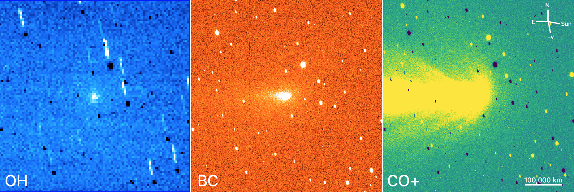
Figure 6: DCT images of OH (left, after dust and ion removal), BC (middle), and CO${}^{+}$ (right, after dust removal). The OH image has been rebinned 8$\times$8 to improve signal to noise. Background stars are visible as trailed streaks in all images, while the negative of background stars (from the continuum image) are also visible in the OH and CO${}^{+}$ images as black trailed streaks. Artifacts from a bad column on the CCD are faintly seen as vertical lines on the BC and CO${}^{+}$ panels. A scale bar and arrows indicating north, east, and the directions to the Sun and the heliocentric velocity vector are given on the CO${}^{+}$ panel.

Our normal procedure for determining gas production rates from fully calibrated images (e.g., KnightSchleicher2015) is to measure the flux in a circular aperture centered on the central condensation and convert to a production rate using a Haser model and standard assumptions about the appropriate lifetimes and scale lengths (AHearn1995). However, we elected to perform a more complex analysis, detailed below, due to several factors. First, the low signal-to-noise of our “pure” OH image meant that trailed stars or their negative residuals from the continuum image which was removed could significantly impact our inferred OH signal. Second, the aforementioned difficulties in decontaminating the image may have potentially led to over- or under-removal of sky background and/or underlying dust continuum. Finally, we identified four lines of CO${}^{+}$ from the A${}^{2}\Pi-\mathrm{X}^{2}\Sigma$ “comet-tail system” (PearseGaydon1976, and references therein) that fall in the OH filter bandpass. While no ion tail structure is evident by eye in our OH image, we were nonetheless concerned about possible ion contamination that was not accounted for in the standard comet filter reduction procedures.
In order to understand the extent to which our “pure” OH image might be contaminated by improperly removed continuum and/or ions, we extracted radial profiles from the uncalibrated CO${}^{+}$, BC, and OH images after removing the background. The radial profiles were binned in distance from the nucleus, $\rho$, and in azimuthal angle, with a resistant mean used to screen out anomalously high or low pixel values. The dust and ion tails were oriented nearly due east, at a position angle (PA) of $\sim$90${}^{\circ}$, slightly offset from the anti-sunward direction of PA = 79${}^{\circ}$, so we determined radial profiles for the sunward and tailward hemispheres as well as 90${}^{\circ}$ wedges centered at 0${}^{\circ}$, 90${}^{\circ}$, 180${}^{\circ}$, and 270${}^{\circ}$. We then fit slopes to the profiles from ${\rho}=4000-60000$ km (the inner radius was set to be about twice the seeing disk). The exact slopes retrieved are very sensitive to the background level, but the behavior of slopes with azimuth is not. The OH slope was the flattest, falling off as roughly ${\rho}^{-0.7}$ in all four quadrants. The BC slope was steeper, falling as roughly ${\rho}^{-1.1}$ in all four quadrants. The CO${}^{+}$ exhibited the steepest slope and was the only one that varied significantly with PA, falling as ${\rho}^{-1.4}$ in the sunward quadrant, and ${\rho}^{-1.0}$ in the other quadrants. The CO${}^{+}$ slopes are consistent with the expected behavior of ions whose sunward extent is minimal, while the consistency of the OH and BC slopes at all PAs suggest that each is relatively free of ion contamination. Furthermore, the more rapid fall off of BC and CO${}^{+}$ compared to OH suggests that, even if there were problems with improper decontamination of the OH image, the flux should increasingly approach the true OH signal at larger distances, with the sunward direction providing the least contaminated OH signal.
This exercise also demonstrated that despite our previous concern about the low signal-to-noise of individual pixels in the OH image, with appropriate binning, clear signal could be detected to at least ${\rho}=1.2{\times}10^{5}$ km. Thus, we measured a radial profile in the sunward quadrant for the “pure” OH image and used this to determine the H${}_{2}$O production rate on the assumption that the coma was spherically symmetric as follows. We created a synthetic OH profile using J. Parker and M. Festou’s online version of the vectorial model (Festou1981) using standard parameters given in Table 2 and scaling for the geometry of R2 PanSTARRS during our observations. We then interpolated the model to the midpoints of our radial profile $\rho$ bins and scaled it up or down to minimize ${\chi}^{2}$ from ${\rho}=4000-1.2{\times}10^{5}$ km. We repeated the process but added a second parameter, a fixed background offset that was allowed to be positive or negative, to minimize ${\chi}^{2}$ again. We continued to add complexity by including the BC and CO${}^{+}$ profiles, first individually and then together, ultimately testing all combinations of vectorial model, fixed background, BC profile, and CO${}^{+}$ profile. We repeated the fitting using an OH image that was flux calibrated with the continuum component set to zero as a further test of the reduction process.
For the DCT imaging, the best-fit using all parameters is a water production rate, $Q$(H${}_{2}$O), of $\sim$3$\times$10${}^{26}$ mol/s. The best-fit for the BC scale factor was close to the solar color, implying that the dust was properly removed in the standard processing despite our earlier concerns. Similarly, the best-fits for both images required a CO${}^{+}$ component, supporting our suspicion that there was some ion contamination. In all cases, the fits yielded $Q$(H${}_{2}$O) between 1 and 5$\times$10${}^{26}$ mol/s, with the largest variations occurring for fits using only background fluxes (e.g., no continuum or ion component). We tested reasonable deviations from the standard vectorial model assumptions, such as varying lifetimes and velocities, but these only changed $Q$(H${}_{2}$O) at the $\sim$20% level or less. The fits consistently show that the OH signal is much stronger than the CO${}^{+}$ and dust continuum beyond $\sim$20,000 km. Figure 7 shows a “pure” OH image using our best-fit parameters (top left panel), the residual flux after removing the modeled OH component from the “pure” OH image (top right), and the radial profiles in our best-fit model (bottom).

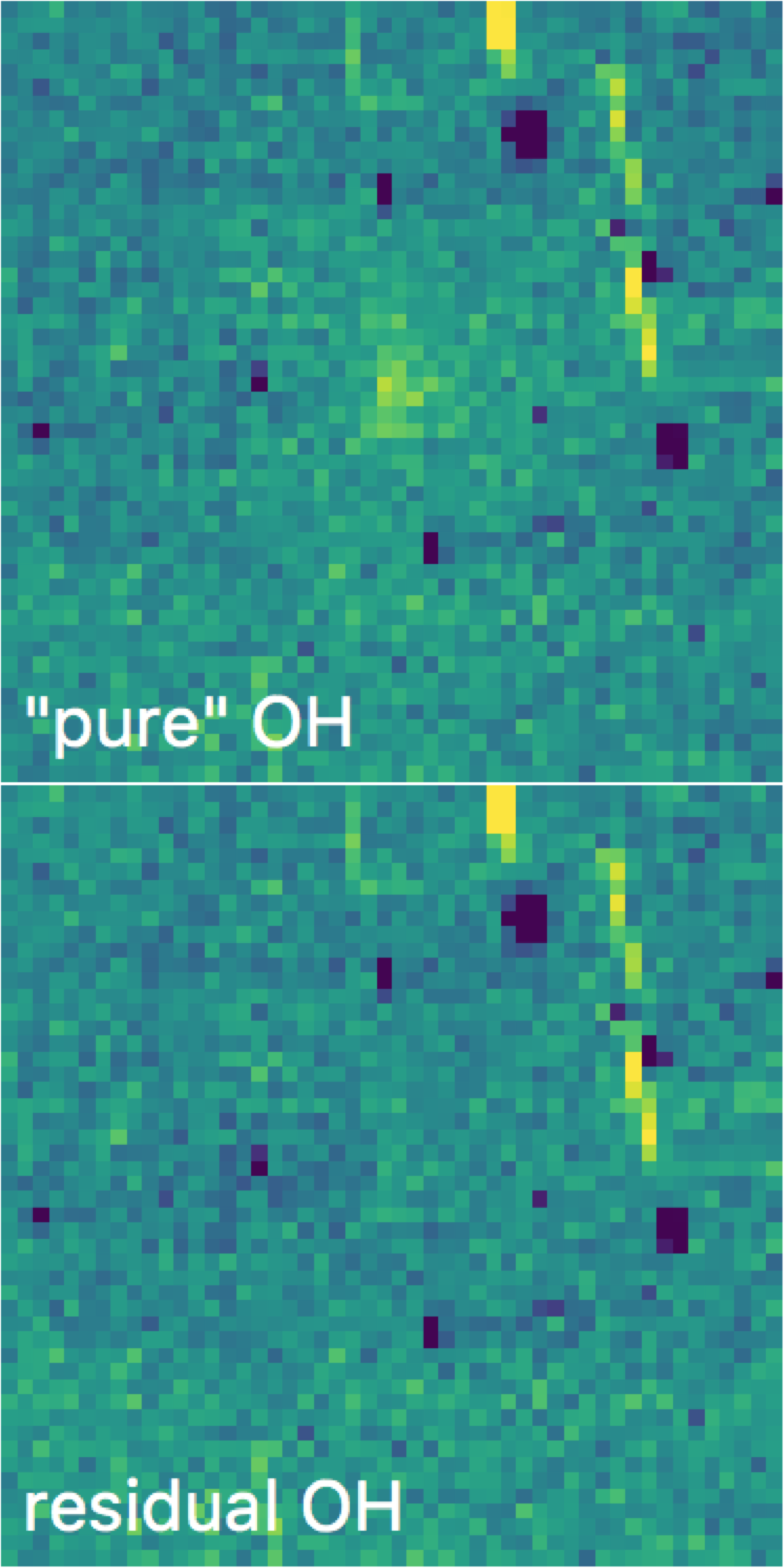
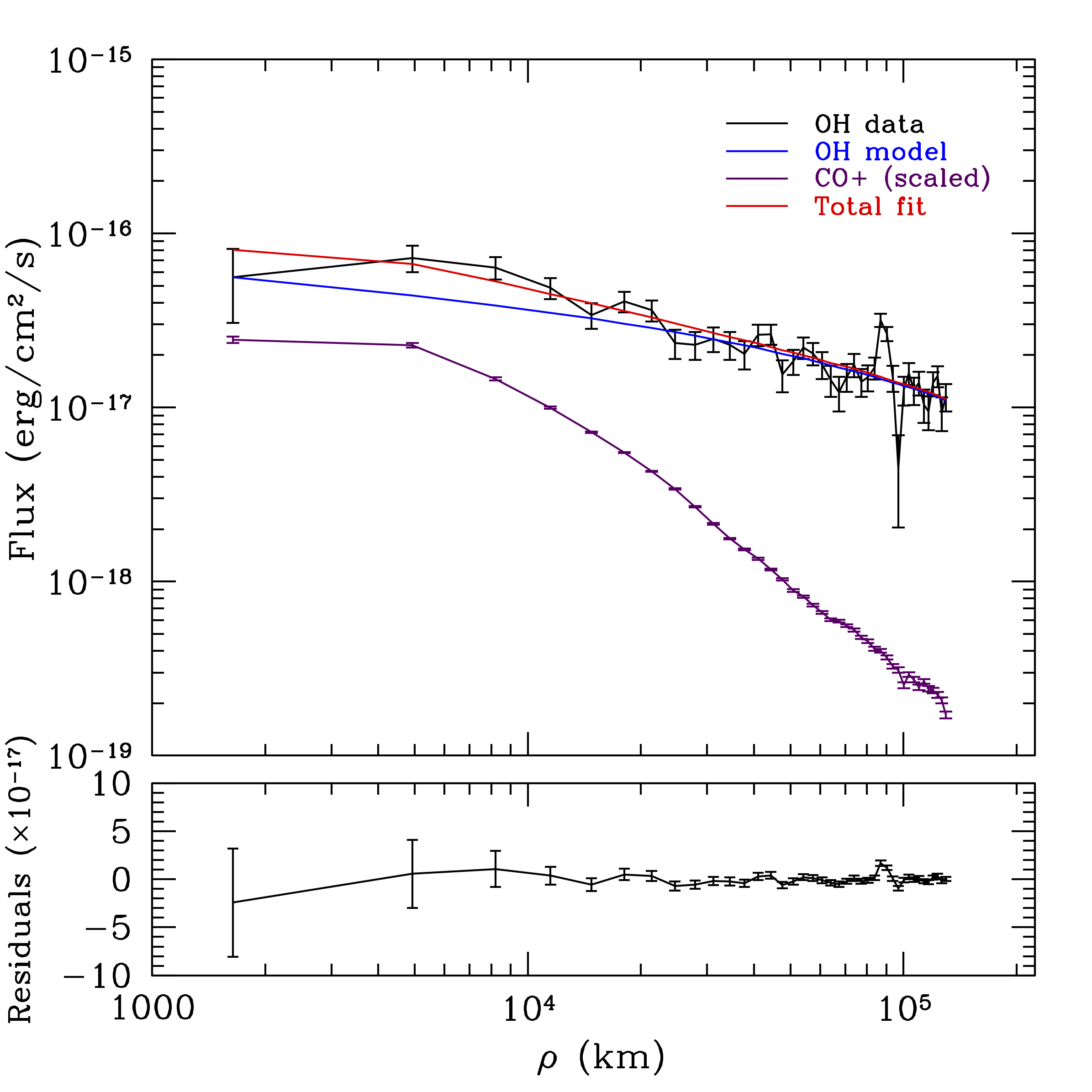
Figure 7: “Pure” OH image produced using the scaling from our best-fit model (top left), residual OH after removing the modeled OH component from the “pure” OH image (top right), and the radial profiles in our best-fit model (bottom). The top panels are zoomed in from the OH image shown in Figure 6, but have the same 8$\times$8 binning applied. They are each $\sim$260,000 km across at the comet, extending just wider than we fit the radial profiles shown in the bottom panel.

The residual OH image has been highly stretched to emphasize subtle features, but shows a hint of over-removal in the tailward direction and slight under-removal of the inner core. Despite the large number of uncertainties and assumptions needed to deal with this unusual comet, we are confident that we have constrained $Q$(H${}_{2}$O) to less than 10${}^{27}$ mol/s with a most likely value of $\sim$(3.1$\pm$0.2)$\times$10${}^{26}$ mol/s (Table LABEL:Qrates). The uncertainty quoted is strictly for our modeled assumptions and does not include systematic uncertainties that are difficult to quantify but could be larger.
Using the observed flux in the BC image we calculated Af$\rho$ as described in Section 3.3, although for the DCT data we used a smaller photometric aperture projected at the comet of 10,000 km, in line with the typical apertures employed by other optical dust photometry observations. We obtain Af$\rho$=561 $\pm$ 6 cm (Table LABEL:Qrates).

3.5 APO-ARCES

Spectra were extracted and calibrated using IRAF scripts that perform bias subtraction, cosmic ray removal, flat fielding, and wavelength calibration. We removed telluric absorption features, the reflected solar continuum from the dust coma, and flux calibrated the spectra employing our standard star observations. We assumed an exponential extinction law and extinction coefficients for APO when flux calibrating the cometary spectra (Hogg2001). More details of our reduction procedures can be found in McKay2012 and CochranCochran2002. We determined slit losses for the flux standard star observations by performing aperture photometry on the slit viewer images as described in McKay2014. Slit losses introduce a systematic error in the flux calibration of $\sim$ 10%.
In our optical spectra we report analysis of five molecular species (N${}_{2}^{+}$, CO${}^{+}$, CN, NH${}_{2}$, C${}_{2}$) and one atomic species (OI). Our analysis of CN, C${}_{2}$, and NH${}_{2}$ employs the same empirical fitting model employed by McKay2014, which utilizes a molecular line list from CochranCochran2002 to fit Gaussian profiles to observed emission features. For N${}_{2}^{+}$ and CO${}^{+}$ we adapt the model from McKay2014 to include CO${}^{+}$ by adding line positions from Kuo1986; Haridass1992; Haridass2000 and N${}_{2}^{+}$ line positions from Dick1978. We integrate over the fits to measure the observed flux. While we detect multiple bands of CO${}^{+}$, we use the (2,0) band for analysis as it has the highest SNR.
For CN, C${}_{2}$, and NH${}_{2}$ these fluxes are converted to production rates using a Haser model in which the input scale lengths are modified to emulate the vectorial model and g-factors from the literature. Molecular lifetimes and g-factors employed are given in Table 2. For [O I], we employ the observed [O I]6300 Å emission as a proxy for H${}_{2}$O production using a similar Haser model (see McKay2012; McKay2014 for more details about the Haser models employed). While [O I]6300 Å emission is often used as a proxy for H${}_{2}$O production in comets, (e.g. Morgenthaler2001; Fink2009; McKay2018), it assumes that H${}_{2}$O is the dominant oxygen-bearing species in the coma, which is not the case for R2 PanSTARRS (see Table LABEL:Qrates).
Ions do not follow a Haser profile. Therefore we do not calculate production rates from derived fluxes for N${}_{2}^{+}$ and CO${}^{+}$, only the relative ratio of N${}_{2}^{+}$/CO${}^{+}$ using

$$\frac{N_{N_{2}^{+}}}{N_{CO^{+}}}=\frac{F_{N_{2}^{+}}}{F_{CO^{+}}}\frac{g_{CO^{+}}}{g_{N_{2}^{+}}}$$ (4)

where $N_{x}$ denotes column density of species $x$, $F_{x}$ is the observed flux of species $x$, and $g_{x}$ is the g-factor for the observed transition of species $x$. The g-factors employed are $g_{CO^{+}}$=3.55 $\times$ 10${}^{-3}$ photons s${}^{-1}$ mol${}^{-1}$ (MagnaniAHearn1986) and $g_{N_{2}^{+}}$=7.00 $\times$ 10${}^{-2}$ photons s${}^{-1}$ mol${}^{-1}$ (Lutz1993).

Table 2:

Parameter Values for Optical Species

Molecule	Parent Lifetime (s)${}^{a}$	Daughter Lifetime (s)${}^{a}$	g-factor (ergs s${}^{-1}$ molecule${}^{-1}$)${}^{a}$
CN	1.3 $\times$ 10${}^{4}$	2.1 $\times$ 10${}^{5}$	2.6 $\times$ 10${}^{-13}$
C2	2.2 $\times$ 10${}^{4}$	6.6 $\times$ 10${}^{4}$	4.5 $\times$ 10${}^{-13}$
NH${}_{2}$	4.1 $\times$ 10${}^{3}$	6.2 $\times$ 10${}^{4}$	6.40 $\times$ 10${}^{-15}$
O I${}^{b}$	8.3 $\times$ 10${}^{4}$	-	-
O I${}^{c}$	1.3 $\times$ 10${}^{5}$	-	-
OH	8.3 $\times$ 10${}^{4}$	1.3 $\times$ 10${}^{5}$	1.54 $\times$ 10${}^{-15}$

${}^{a}$ Given for $r$=1 AU. For CN and OH, given for $\dot{r}$=0 km s${}^{-1}$, but varies with $\dot{r}$.
${}^{b}$ For [O I] from dissociation of H${}_{2}$O into H${}_{2}$ and O; branching ratio employed is 0.07 (BhardwajRaghuram2012)
${}^{c}$ For [O I] from dissociation of OH; branching ratio for H${}_{2}$O to OH + H employed is 0.855 (Huebner1992) and the branching ratio for OH to O + H is 0.094 (BhardwajRaghuram2012).