Chiral Metric Hydrodynamics, Kelvin Circulation Theorem, and the Fractional Quantum Hall Effect

Abstract

By extending the Poisson algebra of ideal hydrodynamics to include a two-index tensor field, we construct a new (2+1)-dimensional hydrodynamic theory that we call “chiral metric hydrodynamics.” The theory breaks spatial parity and contains a degree of freedom which can be interpreted as a dynamical metric, and describes a medium which behaves like a solid at high frequency and a fluid with odd viscosity at low frequency. We derive a version of the Kelvin circulation theorem for the new hydrodynamics, in which the vorticity is replaced by a linear combination of the vorticity and the dynamical Gaussian curvature density. We argue that the chiral metric hydrodynamics, coupled to a dynamical gauge field, correctly describes the long-wavelength dynamics of quantum Hall Jain states with filling factors $\nu=N/(2N+1)$ and $\nu=(N+1)/(2N+1)$ at large $N$. The Kelvin circulation theorem implies a relationship between the electron density and the dynamical Gaussian curvature density. We present a purely algebraic derivation of the low-momentum asymptotics of the static structure factor of the Jain states.

I Introduction

As a general framework, hydrodynamics [1] finds its application in a wide range of physical contexts, including classical systems like classical fluids, gases, or liquid crystals and systems where quantum mechanics plays an important role like superfluids or quantum electronic fluids. Recently, attention has been drawn to systems where the hydrodynamic description manifests features resembling or connected to the topological properties of quantum systems. One example is fluids with odd (or Hall) viscosity [2, 3], which can exist in two spatial dimensions if spatial reflection symmetry is absent. In the most well-known example of such a fluid—the electron fluid in the quantum Hall effect—the odd viscosity is proportional to the shift, a topological property of the quantum Hall states [4]. Another example is fluids of chiral fermions in three dimensions, where the presence of triangle anomalies in the microscopic theory give rise to modifications of the hydrodynamic equations of the finite temperature system, with important physical consequences [5].

In this paper, we describe a theory that we term “chiral metric hydrodynamics”—an extension of the hydrodynamic theory which includes a tensorial degree of freedom, which, for certain purposes, can be interpreted as a dynamical metric. One motivation for considering such a theory is to understand fractional quantum Hall fluids, where the lowest gapped mode is a spin-two mode, the so-called “magnetoroton” [6]. In Ref. [7] it was proposed that the theory governing the dynamics of the magnetoroton at long wavelength is a theory of a dynamical metric, as suggested originally by Haldane [8]. One aim of this work is to relate the ideas of Refs. [8, 7] with the seemingly unrelated picture of a quantum Hall fluid as a fluid of composite fermions obeying a particular form of hydrodynamics [9]. (A phenomenological model that exhibits some features of the theory presented in this paper has been considered in Ref. [10].)

We will first provide a purely mathematical construction of the chiral metric hydrodynamics by enlarging the Poisson algebra of hydrodynamics with the inclusion of a two-index tensor. We will show that, while in general dimensions the resulting theory is simply the theory of elasticity, in two spatial dimensions there is a possibility of a parity-violating Poisson algebra, leading to a theory of a chiral viscoelastic medium which behaves like a solid at high frequencies, but like a fluid with odd viscosity at low frequencies. The hydrodynamic theory describing this medium has interesting features, in particular there is a version of the Kelvin circulation theorem involving a particular linear combination of the vorticity and the density of the Gaussian curvature of the dynamical metric.

Coupling the fluid to a dynamical gauge field, the theory, as we will show, can be used to describe the low-energy dynamics of the fluid of composite fermions in the fractional quantum Hall effect, in particular in the Jain states with filling factors $\nu=N/(2N+1)$ and $\nu=(N+1)/(2N+1)$ at large $N$. By using the Kelvin circulation theorem and the fact that the composite fermion carries an electric dipole moment, we will establish a relationship between the electron density and the dynamical Gaussian curvature density, and use this connection to compute the statics structure factor of quantum Hall state.

II The Poisson algebra

II.1 The Poisson algebra of classical hydrodynamics

We recall that the equations of compressible fluid dynamics can be recasted in the form of Hamilton’s equations of motion of a dynamical system with a Hamiltonian and a set of Poisson brackets. In a normal fluid, the hydrodynamic degrees of freedom are the particle-number density $n(\mathbf{x})$ and the momentum density $\bm{\pi}(\mathbf{x})$. The Poisson brackets between these degrees of freedom are [11]

$$\{\pi_{i}(\mathbf{x}),\,n(\mathbf{y})\} =n(\mathbf{x})\partial_{i}\delta(\mathbf{x}-\mathbf{y}),$$ (1a)

$$\{\pi_{i}(\mathbf{x}),\,\pi_{j}(\mathbf{y})\} =[\pi_{j}(\mathbf{x})\partial_{i}+\pi_{i}(\mathbf{y})\partial_{j}]\delta(\mathbf{x}-\mathbf{y}).$$ (1b)

The Poisson algebra, together with a Hamiltonian in the form of a functional of the hydrodynamic degrees of freedom

$$H=H[n(\mathbf{x}),\pi_{i}(\mathbf{x})],$$ (2)

completely determines the time evolution of the hydrodynamic fields: $\dot{O}=\{H,O\}$, with $O$ being $n$ or $\pi_{i}$. Denoting the variational derivatives of $H$ with respect to $n(\mathbf{x})$ and $\pi_{i}(\mathbf{x})$ by $\mu(\mathbf{x})$ and $v^{i}(\mathbf{x})$, respectively,

$$\delta H=\int\!d\mathbf{x}\left[\mu(\mathbf{x})\delta n(\mathbf{x})+v^{i}(\mathbf{x})\delta\pi_{i}(\mathbf{x})\right],$$ (3)

the equations of motion can be written as

$$\dot{n}+\partial_{i}(nv^{i})=0,$$ (4a)

$$\dot{\pi}_{i}+n\partial_{i}\mu+\pi_{j}\partial_{i}v^{j}+\partial_{j}(v^{j}\pi_{i})=0.$$ (4b)

In the case of a fluid with Galilean invariance, where the Hamilton is the sum of the kinetic and potential energies:

$$H=\int\!d\mathbf{x}\,\left[\frac{\bm{\pi}^{2}}{2mn}+\epsilon(n)\right],$$ (5)

with $m$ being the mass of the fluid particles, Eqs. (4) coincide with the Euler equations for an ideal fluid.

II.2 Poisson algebra and spatial diffeomorphism. Introducing the metric

We will now introduce into the formalism a new hydrodynamic variable—a two-index tensor $G_{ij}$, which will also be called the “metric.” The introduction of a tensor into hydrodynamics makes our theory similar to hydrodynamics of nematic liquid crystals, for which the Poisson bracket formalism has been applied [12]. Here we first abstract ourselves from physical applications and construct our theory from purely mathematical consideration.

First, we note that the momentum density $\bm{\pi}(\mathbf{x})$ can be regarded as the operator generating infinitesimal diffeomorphism transformation [13]. More concretely, if one defines for each vector field $\xi^{k}(\mathbf{x})$ the quantity

$$\hat{\xi}=\int\!d\mathbf{y}\,\xi^{k}(\mathbf{y})\pi_{k}(\mathbf{y}),$$ (6)

then the Poisson brackets of $\hat{\xi}$ with $n$ and $\pi_{i}$,

$$\{\hat{\xi},\,n(\mathbf{x})\} =-\xi^{k}\partial_{k}n-n\partial_{k}\xi^{k},$$ (7a)

$$\{\hat{\xi},\,\pi_{i}(\mathbf{x})\} =-\xi^{k}\partial_{k}\pi_{i}-\pi_{k}\partial_{i}\xi^{k}-\xi_{i}\partial_{k}\xi^{k},$$ (7b)

reproduce exactly the shift of a scalar density and a covariant vector density (both carrying weight $w=1$) under an infinitesimal coordinate transformation $x^{k}\to x^{k}+\xi^{k}$, and can be written compactly through the Lie derivative:

$$\{\hat{\xi},\,O(\mathbf{x})\}=\pounds_{\xi}O,\qquad O=n,\pi_{i}$$ (8)

In other words, the Poisson algebra formed by $\pi_{i}(\mathbf{x})$ is isomorphic to the algebra of spatial diffeomorphism, and the Poisson bracket of $\pi_{i}$ with any quantity is determined by the law of transformation of the latter under diffeomorphism. For example, the momentum per particle $u_{i}=\pi_{i}/n$ is a vector, and this is manifested in its Poisson bracket with the momentum density:

$$\{\hat{\xi},\,u_{i}(\mathbf{x})\}=-\xi^{k}\partial_{k}u_{i}-u_{k}\partial_{i}\xi^{k}=-\pounds_{\xi}u_{i}\,.$$ (9)

We are now ready to introduce a new degree of freedom into the theory: the metric $G_{ij}$. It is symmetric, $G_{ij}=G_{ji}$, and we chose it transform as a covariant tensor, which means

$$\{\hat{\xi},\,G_{ij}(\mathbf{x})\}=-\pounds_{\xi}G_{ij}=-\xi^{k}\partial_{k}G_{ij}-G_{kj}\partial_{i}\xi^{k}-G_{ik}\partial_{j}\xi^{k}.$$ (10)

This condition fixes the Poisson bracket between $\pi_{i}$ and $G_{ij}$,

$$\{G_{ij}(\mathbf{x}),\,\pi_{k}(\mathbf{y})\}=\left[G_{ik}(\mathbf{x})\partial_{j}+G_{jk}(\mathbf{x})\partial_{i}+\partial_{k}G_{ij}(\mathbf{x})\right]\delta(\mathbf{x}-\mathbf{y}).$$ (11)

Note that this is quite different from the corresponding Poisson bracket in the theory of nematic liquid crystals [12].

As in general relativity, we will denote the matrix inverse of $G_{ij}$ as $G^{ij}$ and $\det G_{ij}$ as $G$. Note that $G$ transforms like a scalar density, i.e., in the same way as $n$. Thus it is consistent to impose the constraint $\sqrt{G}=n$. This means that beside $n$ and $\bm{\pi}$, the new dynamical degrees of freedom form a unimodular matrix $G_{ij}/n^{2/d}$, where $d$ is the number of spatial dimensions.

To complete the Poisson algebra, we need to define the Poisson brackets between $G_{ij}$ and $n$, and between the components of $G_{ij}$. For the Poisson bracket between $G$ and $n$ the simplest choice is to declare it to vanish:

$$\{G_{ij}(\mathbf{x}),\,n(\mathbf{y})\}=0.$$ (12)

As to the Poisson bracket between components of $G_{ij}$, there are two different natural choices that lead to dramatically different hydrodynamic theories. The simpler choice, which works in any number of spatial dimensions, is to take the Poisson brackets between the metric components to be zero,

$$\{G_{ij}(\mathbf{x}),\,G_{kl}(\mathbf{y})\}=0.$$ (13)

However, in this case our hydrodynamic theory is simply another formulation of the theory of elasticity. This can be seen as follows. Assume the most general Hamiltonian $H=H[n(\mathbf{x}),\pi_{i}(\mathbf{x}),G_{ij}(\mathbf{x})]$ and introducing again its functional derivatives,

$$\delta H=\int\!d\mathbf{x}\,\left[\mu(\mathbf{x})\delta n(\mathbf{x})+v^{i}(\mathbf{x})\delta\pi_{i}(\mathbf{x})+\frac{1}{2}\sigma^{ij}(\mathbf{x})\delta G_{ij}(\mathbf{x})\right],$$ (14)

the equations of motion have the form

$$\partial_{t}n =-\partial_{i}(nv^{i}),$$ (15a)

$$\partial_{t}\pi_{i} =-n\partial_{i}\mu-\pi_{j}\partial_{i}v^{j}-\partial_{j}(v^{j}\pi_{i})-\partial_{j}(\sigma^{jk}G_{ki})+\frac{1}{2}\sigma^{jk}\partial_{i}G_{jk}\,,$$ (15b)

$$\partial_{t}G_{ij} =-v^{k}\partial_{k}G_{ij}-G_{ik}\partial_{j}v^{k}-G_{jk}\partial_{i}v^{k}.$$ (15c)

In particular, Eq. (15c) means that the metric tensor is frozen into the fluid, and is given simply by the shape of an initially spherical droplet advected by the flow. The fact that the energy depends on the shape of this droplet means that we are dealing not with fluid, but with an elastic solid, where $\sigma^{ij}$ is basically the elastic stress. This finding can be confirmed, for example, by finding the normal modes of the linearized hydrodynamic equations: one finds, in addition to the longitudinal sound, the transverse sound.

III Chiral Poisson algebra and chiral metric hydrodynamics

III.1 Construction of the chiral metric hydrodynamic theory

In two spatial dimensions, if one does not impose spatial parity, then there is another choice for the Poisson bracket between $G_{ij}$:

$$\{G_{ij}(\mathbf{x}),\,G_{kl}(\mathbf{y})\}=-\frac{1}{s}\left(\epsilon_{ik}G_{jl}+\epsilon_{il}G_{jk}+\epsilon_{jk}G_{il}+\epsilon_{jl}G_{ik}\right)\delta(\mathbf{x}-\mathbf{y}),$$ (16)

where $s$ is a pure number, and $\epsilon_{ij}=-\epsilon_{ji}$, $\epsilon_{12}=1$. One needs to verify that the Jacobi identity is satisfied. Excluding the delta-function on the right-hand side, Eq. (16) has the same form as the commutators of the $\mathfrak{sl}(2,\mathbb{R})$ algebra. That means that the Jacobi identity $\{\{G,G\},G\}+\cdots=0$ is satisfied. Checking the Jacobi identity $\{\pi,\{G,G\}\}+\cdots=0$ is equivalent to verifying that the two sides of Eq. (16) transform in the same way under general coordinate transformations. This can be established by noting that $\delta(\mathbf{x}-\mathbf{y})$ is a scalar density of weight $-1$ and $\epsilon_{ij}$ a tensor density of weight $+1$. Other cases can be checked trivially.

Given the Hamiltonian $H=H[n(\mathbf{x}),\pi_{i}(\mathbf{x}),G_{ij}(\mathbf{x})]$, the hydrodynamic equations can be now written down using the conjugate variables defined in Eq. (14):

$$\partial_{t}n =-\partial_{i}(nv^{i}),$$ (17a)

$$\partial_{t}\pi_{i} =-n\partial_{i}\mu-\pi_{j}\partial_{i}v^{j}-\partial_{j}(v^{j}\pi_{i})-\partial_{j}(\sigma^{jk}G_{ki})+\frac{1}{2}\sigma^{jk}\partial_{i}G_{jk}\,,$$ (17b)

$$\partial_{t}G_{ij} =-v^{k}\partial_{k}G_{ij}-G_{ik}\partial_{j}v^{k}-G_{jk}\partial_{i}v^{k}+\frac{1}{s}(\epsilon_{ik}G_{jl}+\epsilon_{jk}G_{il})\sigma^{kl}.$$ (17c)

Compared to Eqs. (15), the equation for time evolution of the metric contains a parity-odd term.

If the metric tensor $G_{ij}$ is almost isotropic, like in most applications that we will consider, then one can expand

$$G_{ij}=n(\delta_{ij}+Q_{ij}),\qquad Q_{ij}\ll 1,~{}Q_{ii}=0.$$ (18)

In this limit, one can use the “reduced” Poisson brackets

$$\{Q_{ij}(\mathbf{x}),\,\pi_{k}(\mathbf{y})\} =(\delta_{ik}\partial_{j}+\delta_{jk}\partial_{i}-\delta_{ij}\partial_{k})\delta(\mathbf{x}-\mathbf{y}),$$ (19)

$$\{Q_{ij}(\mathbf{x}),\,Q_{kl}(\mathbf{y})\} =-\frac{1}{sn}(\epsilon_{ik}\delta_{jl}+\epsilon_{il}\delta_{jk}+\epsilon_{jk}\delta_{il}+\epsilon_{jl}\delta_{ik})\delta(\mathbf{x}-\mathbf{y}),$$ (20)

to derive the hydrodynamic equations

$$\partial_{t}n+\partial_{i}(nv^{i})=0,$$ (21)

$$\partial_{t}\pi_{i}+\partial_{j}(v^{j}\pi_{i})+n\partial_{i}\mu+\pi_{j}\partial_{i}v^{j}+\partial_{j}\tau^{ji}=0,$$ (22)

$$\partial_{t}Q_{ij}-\frac{1}{sn}(\epsilon_{ik}\tau_{kj}+\epsilon_{jk}\tau_{ki})+V_{ij}=0,$$ (23)

where $\tau^{ij}=n\sigma^{ij}$ and

$$V_{ij}=\partial_{i}v_{j}+\partial_{j}v_{i}-\delta_{ij}\bm{\nabla}\cdot\mathbf{v}.$$ (24)

Note that in the equation for momentum conservation $\tau^{ij}$ plays the role of an anisotropic stress.

III.2 The high- and low-frequency regimes

Ignoring for a moment the $V_{ij}$ term, if one introduces the “Lamé coefficient” $\tilde{\mu}$ so that $\tau^{ij}=\tilde{\mu}Q_{ij}$, the equation for $Q_{ij}$

$$\partial_{t}Q_{ij}=\frac{\tilde{\mu}}{ns}(\epsilon_{ik}Q_{kj}+\epsilon_{jk}Q_{ki}),$$ (25)

means that the metric tensor rotates in the space $(Q_{xx},Q_{xy})$ with angular velocity

$$\omega_{Q}=\frac{2\tilde{\mu}}{ns}\,.$$ (26)

If the upper range of validity of our hydrodynamic theory is much larger than $\omega_{Q}$, then one can talk about the high-frequency ($\omega\gg\omega_{Q}$) and low-frequency ($\omega\ll\omega_{Q}$) regimes. In the former regime Eq. (23) becomes $\partial_{t}Q_{ij}+V_{ij}=0$, which can be solved in terms of the displacement $u_{i}$, defined so that $v_{i}=\dot{u}_{i}$:

$$Q_{ij}=-(\partial_{i}u_{j}+\partial_{j}u_{i}-\delta_{ij}\partial_{k}u_{k}),$$ (27)

and Eq. (22) becomes the equation of motion of an elastic medium with $\tilde{\mu}$ being a Young modulus.

In the low-frequency regime $\omega\ll\omega_{Q}$, Eq. (23) reduces to the balance of the last two terms:

$$-\frac{1}{sn}(\epsilon_{ik}\tau_{kj}+\epsilon_{jk}\tau_{ki})+V_{ij}=0,$$ (28)

whose solution is

$$\tau^{ij}=-\frac{sn}{4}\left(\epsilon_{ik}V_{kj}+\epsilon_{jk}V_{ik}\right).$$ (29)

But $\tau^{ij}$ appears as a contribution to the stress tensor in momentum conservation (22). This means the fluid has a nonzero odd (or Hall) viscosity equal to

$$\eta^{H}=\frac{sn}{2}\,.$$ (30)

Following Ref. [4], $s$ can then be identified with the average orbital spin per particle.

III.3 The Kelvin circulation theorem in chiral metric hydrodynamics

In ordinary ideal hydrodynamics, there exist an infinite number of conserved quantities

$$I_{F}=\int\!d\mathbf{x}\,n(\mathbf{x})F\left(\frac{\omega(\mathbf{x})}{n(\mathbf{x})}\right),$$ (31)

where

$$\omega=\epsilon^{ij}\partial_{i}u_{j}\equiv\epsilon^{ij}\partial_{i}\left(\frac{\pi_{j}}{n}\right).$$ (32)

will be called “vorticity,” and $F$ is an arbitrary function of its argument. The conservation of these charges does not depend on the Hamiltonian: $I_{F}$ has zero Poisson brackets with all hydrodynamics variables, i.e., $n$ and $\pi_{i}$. In other words, $I_{F}$ are Casimirs of the Poisson algebra. This can established from the Poisson brackets

$$\{n(\mathbf{x}),\,\omega(\mathbf{y})\} =0,$$ (33)

$$\{\pi_{i}(\mathbf{x}),\,\omega(\mathbf{y})\} =\omega(\mathbf{x})\partial_{i}\delta(\mathbf{x}-\mathbf{y}),$$ (34)

which follow from Eq. (1). The second Poisson bracket (34) is equivalent to the statement that $\omega(\mathbf{x})$ transform like a scalar density, which can already be seen from Eq. (32). The time evolution of $\omega$ has the form of a conservation law:

$$\partial_{t}\omega+\partial_{i}(\omega v^{i})=0.$$ (35)

from which the conservation of (31) also follows.

In metric hydrodynamics $I_{F}$ are no longer Casimirs: the Poisson bracket of the vorticity with the metric $G_{ij}$ is nonzero. It turns out, however, that within the chiral metric hydrodynamic theory there exists a modified version of the Kelvin circulation theorem. To find it we need to find a generalized vorticity $\Omega(\mathbf{x})$ that commutes with the density and the metric, and at the same time transforms like a scalar density:

$$\{n(\mathbf{x}),\,\Omega(\mathbf{y})\} =0,$$ (36a)

$$\{\pi_{i}(\mathbf{x}),\,\Omega(\mathbf{y})\} =\Omega(\mathbf{x})\partial_{i}\delta(\mathbf{x}-\mathbf{y}),$$ (36b)

$$\{G_{ij}(\mathbf{x}),\,\Omega(\mathbf{y})\} =0.$$ (36c)

To satisfy Eqs. (36a) and (36b), one can add to $\omega$ a scalar density constructed from the metric. This scalar density must be chosen so that the resulting $\Omega$ has zero Poisson bracket with the metric. Since $\{\omega,G\}$ contains two spatial derivatives and $\{G,G\}$ has no derivative, this scalar density has to contain two derivatives. The only scalar density that one can construct from $G_{ij}$ and two derivatives is $\sqrt{G}\,R[G]$ where $R[G]$ is the scalar Gaussian curvature constructed from the metric $G_{ij}$. By a direct check one can verify that the combination

$$\Omega=\omega+\frac{s}{2}\sqrt{G}\,R[G]$$ (37)

satisfies Eq. (36c). Calculation is facilitated by working in the coordinate systems where $G_{ij}=\delta_{ij}+\delta G_{ij}$ where $\delta G_{ij}$ is small in the vicinity of the point under consideration. Hence $\Omega$ is advected by the flow:

$$\partial_{t}\Omega+\partial_{i}(\Omega v^{i})=0.$$ (38)

In a later part of the paper, we will consider the application of chiral metric hydrodynamics to the fractional quantum Hall states, in which the fluid is coupled to a U(1) gauge field $a_{\mu}$. To find a generalization of the Kelvin circulation theorem in that case, one notes that the equation of momentum conservation is modified by the Lorentz force term:

$$\partial_{t}\pi_{i}=n(e_{i}+\epsilon_{ij}v^{j}b)-n\partial_{i}\mu-\pi_{j}\partial_{i}v^{j}-\partial_{j}(v^{j}\pi_{i})-\partial_{j}(\sigma^{jk}G_{ki})+\frac{1}{2}\sigma^{jk}\partial_{i}G_{jk}\,.$$ (39)

where $e_{i}=\partial_{i}a_{0}-\partial_{0}a_{i}$ and $b=\epsilon^{ij}\partial_{i}a_{j}$. One can easily check that if one redefines the generalized vorticity as

$$\Omega=b+\omega+\frac{s}{2}\sqrt{G}R[G],$$ (40)

then it will continue to satisfy the conservation law (38). Hence the quantities (31) remain conserved.

Another, more formal way is to consider the enlarged Poisson algebra with the gauge potential $a_{i}(\mathbf{x})$ and its canonical conjugate momentum $\pi_{a_{i}}(\mathbf{x})$ as new fields. In the presence of a gauge field, the Poisson bracket between $\pi_{i}$ is modified

$$\{\pi_{i}(\mathbf{x}),\,\pi_{j}(\mathbf{y})\}=[\pi_{j}(\mathbf{x})\partial_{i}+\pi_{i}(\mathbf{y})\partial_{j}]\delta(\mathbf{x}-\mathbf{y})-\epsilon_{ij}b(\mathbf{x})n(\mathbf{x})\delta(\mathbf{x}-\mathbf{y}),$$ (41)

and two additional nontrivial Poisson brackets arise:

$$\{\pi_{a_{i}}(\mathbf{x}),\,a_{j}(\mathbf{y})\} =\delta_{ij}\delta(\mathbf{x}-\mathbf{y}),$$ (42)

$$\{\pi_{a_{i}}(\mathbf{x}),\,\pi_{j}(\mathbf{y})\} =-\delta_{ij}n(\mathbf{x})\delta(\mathbf{x}-\mathbf{y}).$$ (43)

One can then check that $\Omega$ defined in Eq. (40) satisfies Eqs. (36) and has zero Poisson brackets with both $a_{i}$ and $\pi_{a_{i}}$.

IV Chiral metric hydrodynamics of the fractional quantum Hall fluid

IV.1 Review of the Dirac composite fermion theory

We now apply chiral metric hydrodynamics to describe fractional quantum Hall fluids [14, 15]. Let us recall the simplest formulation of the problem: a system of interacting nonrelativistic electrons, moving in the $xy$ plane in a magnetic field $B$ such that the density of electrons $\rho_{\rm e}$ is smaller than the density of states on the lowest Landau level $B/2\pi$. (Here we absorb the factor $-|e|/c$ into the magnetic field. In the normal convention the magnetic field directed is opposite to the $z$-axis, after absorbing this factor it is directed along the $z$-axis. We use the unit system where $\hbar=1$ and define the magnetic length $\ell_{\rm B}=1/\sqrt{B}$.)

The most nontrivial feature of the quantum Hall fluids is that the low-energy quasiparticle is completely different from the electron. According to the composite fermion picture [16, 17, 18, 19], near half filling, where the filling factor $\nu=2\pi\rho_{\rm e}/B\approx\frac{1}{2}$, the quasiparticle is the composite fermion, which interacts with a dynamical gauge field $a_{\mu}$. The dynamic magnetic field has expectation value

$$\langle b\rangle=B-4\pi\rho_{\rm e}\,.$$ (44)

At $\nu=\frac{1}{2}$ the average dynamical magnetic field is zero and the composite fermions form a Fermi liquid.

In the lowest Landau level limit ($B\to\infty$ at fixed $\nu$, or purely theoretically, when the electron mass goes to zero), particle-hole symmetry becomes an exact symmetry. In this case the composite fermion is a massless Dirac fermion with Berry phase of $\pi$ around the Fermi line [20]. The composite fermion has density $n=B/4\pi$. This is close to, but in general not equal to the density of the electron $\rho_{\rm e}$. The composite fermion is electrically neutral but carries a nonzero electric dipole moment $\mathbf{d}$ perpendicular and proportional to its momentum: $\mathbf{d}=-\ell_{\rm B}^{2}\mathbf{p}\times\mathbf{\hat{z}}$.

We will consider the so-called Jain states, which form two series converging to $\nu=\frac{1}{2}$,

$$\nu=\frac{N}{2N+1}\,,\qquad\nu=\frac{N+1}{2N+1}\,,\qquad N=1,2,3,\ldots$$ (45)

The $N=1$ case is the Laughlin $\nu=\frac{1}{3}$ state and its particle-hole conjugate $\nu=\frac{2}{3}$, but we will be mostly interested in the limit of large $N$, $N\gg 1$. On the Jain states, the dynamical magnetic field has nonzero average,

$$\langle b\rangle=\pm\frac{B}{2N+1}\,.$$ (46)

IV.2 Microscopic derivation of the Poisson algebra

We now argue that at sufficiently long wavelength the quantum Hall system is described by chiral metric hydrodynamics. The reason is the following. For large $N$ one can treat the system as a Fermi liquid in a small magnetic field. In the bosonized approach [21, 22] the dynamics of the Fermi surface can be parameterized through an infinite number of scalar fields (called $u_{n}$ in Ref. [23]), one field per spin. Now in the regime $\omega\gg v_{F}q$, where $v_{F}$ is the Fermi velocity, one can truncate the tower of scalar fields to a few first fields. This is because at zero momentum these fields cannot mix with each other due to the conservation of momentum, and the strength of the mixing is governed by the parameter $v_{F}q/\omega$. This is essentially the reason the longitudinal and transverse zero sounds in Fermi liquid with large Landau parameter $F_{1}$ (and $F_{\ell}\sim 1$ with $\ell\geq 2$) can be described by a theory of elasticity [24, 25].

In the fractional quantum Hall case the dynamical magnetic field has a nonzero average value $\langle b\rangle=\pm B/(2N+1)$, in which the composite fermions form a integer quantum Hall state with a gap of order $\Delta\sim b/m_{*}=v_{F}b/p_{F}$. In our gapped phase $\omega\sim\Delta$ and the mixing is small when $q\ell_{B}\ll 1/N$. In this regime one can limit ourselves fields of lowest spins. In practice, this means spins less or equal to 2.

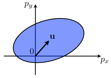
Figure 1: An elliptical Fermi surface.

We assume then that the Fermi surface has the shape of an ellipse (Fig. 1). One can completely characterize the ellipse by the moments of the distribution function $f(\mathbf{x},\mathbf{p})$, which is 1 inside the ellipse and 0 outside.

$$n(\mathbf{x}) =\int\!\frac{d\mathbf{p}}{(2\pi)^{2}}\,f(\mathbf{x},\mathbf{p}),$$ (47)

$$\pi_{i}(\mathbf{x}) =\int\!\frac{d\mathbf{p}}{(2\pi)^{2}}\,p_{i}f(\mathbf{x},\mathbf{p}),$$ (48)

$$G_{ij}(\mathbf{x}) =\frac{1}{\pi n(\mathbf{x})}\left(\int\!\frac{d\mathbf{p}}{(2\pi)^{2}}\,p_{i}p_{j}f(\mathbf{x},\mathbf{p})-\frac{\pi_{i}(\mathbf{x})\pi_{j}(\mathbf{x})}{n(\mathbf{x})}\right).$$ (49)

The tensor $G_{ij}$ is defined in such a way that $\sqrt{\det G}=n$. The Poisson bracket between the fields can then be evaluate from the following semiclassical prescription: for any two functions $A(\mathbf{x},\mathbf{p})$ and $B(\mathbf{x},\mathbf{p})$ on the phase phase,

$$\left\{\int\!\frac{d\mathbf{x}\,d\mathbf{p}}{(2\pi)^{d}}\,A(\mathbf{x},\mathbf{p})f(\mathbf{x},\mathbf{p}),\,\int\!\frac{d\mathbf{x}\,d\mathbf{p}}{(2\pi)^{d}}\,B(\mathbf{x},\mathbf{p})f(\mathbf{x},\mathbf{p})\right\}=\int\!\frac{d\mathbf{x}\,d\mathbf{p}}{(2\pi)^{d}}\,\{A,B\}(\mathbf{x},\mathbf{p})f(\mathbf{x},\mathbf{p}),$$ (50)

where $\{A,\,B\}$ is the classical Poisson bracket [26]

$$\{A,\,B\}=\frac{\partial A}{\partial p_{i}}\frac{\partial B}{\partial x^{i}}-\frac{\partial A}{\partial x^{i}}\frac{\partial B}{\partial p_{i}}-\epsilon_{ij}b\frac{\partial A}{\partial p_{i}}\frac{\partial B}{\partial p_{j}}\,.$$ (51)

Following this prescription, we find that all the Poisson brackets, except $\{G,\,G\}$, can be expressed in terms of the hydrodynamic variables, and coincide with the expressions postulated in the hydrodynamic theory. On the other hand the Poisson bracket $\{G,\,G\}$ contains the third moment of the distribution function $\int_{p}p_{i}p_{j}p_{k}f$; assuming the Fermi surface has the shape of an ellipse, this third moment can be expressed in terms of the lower moments,

$$\int\!\frac{d\mathbf{p}}{(2\pi)^{2}}\,p_{i}p_{j}p_{k}f(\mathbf{x},\mathbf{p})=\frac{\pi_{i}\pi_{j}\pi_{k}}{n^{2}}+\pi(\pi_{i}G_{jk}+\pi_{j}G_{ik}+\pi_{k}G_{ij}).$$ (52)

At the end of a lengthy, but straightforward, calculation, one finds

$$\{G_{ij}(\mathbf{x}),\,G_{kl}(\mathbf{y})\}=-\frac{b+\omega}{\pi n}(\epsilon_{ik}G_{jl}+\epsilon_{il}G_{jk}+\epsilon_{jk}G_{il}+\epsilon_{jk}G_{ik})\delta(\mathbf{x}-\mathbf{y}).$$ (53)

This is very similar to, but not exactly, Eq. (16): the constant factor $1/s$ there is replaced by $(b+\omega)/\pi n$, which is a dynamical field. If one replaces this prefactor by its expectation value,

$$\frac{b+\omega}{\pi n}\to\frac{\langle b\rangle}{\pi n}=\begin{cases}\displaystyle{\phantom{+}\frac{4}{2N+1}}\,,&\nu=\displaystyle{\frac{N}{2N+1}}\,,\vspace{6pt}\\ \displaystyle{-\frac{4}{2N+1}}\,,&\nu=\displaystyle{\frac{N+1}{2N+1}}\,,\end{cases}$$ (54)

then one can identify

$$s=\pm\frac{1}{2}\left(N+\frac{1}{2}\right),$$ (55)

where the upper and lower signs correspond to $\nu=N/(2N+1)$ and $\nu=(N+1)/(2N+1)$, respectively. The replacement can also be justified by the following argument: up to terms containing second derivatives of $G_{ij}$, the prefactor is $\Omega/n$, which in the chiral metric hydrodynamics is conserved and determined completely by the initial condition. Provided that at infinite past the system is in the ground state, $\Omega/n$ is then equal to $\langle b\rangle/n$. Note that our semiclassical prescription for computing the Poisson bracket, Eqs. (50) and (51), cannot in principle yield terms with second derivatives; one may hope a more sophisticated treatment will reveal their existence. In any case, for the calculation of linear response, the replacement (54) can always be made.

One may be concerned that the parameter $s$ in Eq (55), which has been previously identified with the orbital spin per particle, is neither integer nor half-integer. This is not a problem, as $s$ is the average orbital angular momentum per particle. This suggests another way to determine $s$. Recall that in the composite fermion picture, the $\nu=N/(2N+1)$ state has the composite fermions filling up $N+\frac{1}{2}$ Landau levels: half of the zero-energy Landau level ($n=0$) and the positive-energy levels with quantum numbers $n=1,2,\ldots,N$. Now the orbital spin of a particle on the $n$-th Landau level is $n$, so the average orbital spin is

$$s=\frac{1}{N+\frac{1}{2}}\left(\frac{1}{2}\cdot 0+1+2+\cdots+N\right)=\frac{N(N+1)}{2N+1}\,.$$ (56)

For the $\nu=(N+1)/(2N+1)$ state, $s$ flips sign. The value in Eq. (56) does not coincides with that in Eq. (55), but the relative difference is of order $1/N^{2}$ at large $N$. This discrepancy is should be attributed to the imperfectness of the semiclassical procedure (50). We thus conjecture that (56) represents the exact value of the parameter $s$ and use it in later calculations. Note that even for $N=1$ the values of the $s$ in Eqs. (55) and (56) differ from each other only by a factor of 9/8.

From Eq. (30) and (56) one can find the odd viscosity of the Hall fluid,

$$\eta^{H}=\pm\frac{N(N+1)}{2N+1}\frac{B}{8\pi}\,.$$ (57)

This should be compared with the expectation: $\eta^{H}=\frac{1}{4}\rho_{\rm e}(\mathcal{S}-1)$ where $\mathcal{S}$ is the shift, and $\mathcal{S}-1$ is the part of the shift associated with the guiding centers. Equation (57) exactly matches this expectation, given that $\mathcal{S}=N+2$ for $\nu=N/(2N+1)$ and $\mathcal{S}=-N+1$ for $\nu=(N+1)/(2N+1)$.

IV.3 Equations of motion of chiral metric hydrodynamics of fractional quantum Hall states

We now derive the relevant formulas for the metric hydrodynamics of the composite fermions. Due to the dipolar interaction of the composite fermion with the external electric field, the Hamiltonian of the composite fermion fluid contains a term which can be viewed as a source term for the momentum density

$$H=H_{0}[n,\pi_{i},G_{ij},b]+\int\!d\mathbf{x}\left(-a_{0}(\mathbf{x})n(\mathbf{x})+V^{i}(\mathbf{x})\pi_{i}(\mathbf{x})\right),$$ (58)

where $V^{i}=\epsilon^{ij}E_{j}/B$ is the drift velocity created by the external electric field. This Hamiltonian transforms correctly under Galilean boosts. The lowest Landau level limit is the limit of massless electrons, so the total momentum $\mathbf{P}$ is invariant under Galilean boosts, while the total energy should transform as

$$H\to H-\bm{\beta}\cdot\mathbf{P},$$ (59)

when going from a frame $K$ to a frame $K^{\prime}$ moving with velocity $\bm{\beta}$ with respect to $K$. This is exactly what happens with the Hamiltonian (58): under boosts all variables remain invariant except for the external electric field which transforms as $\mathbf{E}\to\mathbf{E}+\bm{\beta}\times\mathbf{B}$, implying $V^{i}\to V^{i}-\beta^{i}$ and (59).

In the Dirac composite fermion theory, the dynamical gauge field $a_{\mu}$ appears in the action as Lagrange multipliers enforcing constraints of the form

$$n-\frac{B}{4\pi} =0,$$ (60a)

$$nv^{i}-\epsilon^{ij}\partial_{j}\frac{\delta H_{0}}{\delta b} =0.$$ (60b)

The equations for the hydrodynamic variables coincide with those of metric hydrodynamics in an electromagnetic field with [Eqs. (17a), (17c), and (39)], but with the replacement $v^{i}\to\nu^{i}=v^{i}+V^{i}$.

$$\partial_{t}n+\partial_{i}(n\nu^{i})=0,\qquad\nu^{i}=v^{i}+\frac{\epsilon^{ij}E_{j}}{B}\,,$$ (61)

$$\partial_{t}\pi_{i}+n\partial_{i}\mu+\pi_{j}\partial_{i}\nu^{j}+\partial_{j}(\nu^{j}\pi_{i})+\partial_{j}(\sigma^{jk}G_{ki})-\frac{1}{2}\sigma^{jk}\partial_{i}G_{jk}=ne_{i}+n\epsilon_{ij}\nu^{j}b,$$ (62)

$$\partial_{t}G_{ij}+\pounds_{\nu}G_{ij}-\frac{1}{s}(\epsilon_{ik}G_{jl}+\epsilon_{jk}G_{il})\sigma^{kl}=0.$$ (63)

The problem of finding the response of the quantum Hall fluid to external electromagnetic perturbation reduces to the finding the solution to the hydrodynamic equations and the constraint equations in the background $E$ and $B$ fields. [Note that, due to the constraints (60), Eq. (61) is satisfied automatically.]

After the solution has been found, the electron density should be read from

$$\rho_{\rm e}=\frac{\delta S}{\delta A_{0}}=\frac{B-b}{4\pi}-\epsilon^{ij}\partial_{i}\left(\frac{\pi_{j}}{B}\right).$$ (64)

By using the constraint (60a), this expression can be rewritten as

$$\rho_{\rm e}=\frac{1}{4\pi}(B-b-\omega),$$ (65)

where $\omega$ is the vorticity defined in Eq. (32). One can also compute the electron current density from $j^{i}_{\rm e}=\delta S/\delta A_{i}$, but the formulas are somewhat cumbersome and will not be presented here.

Two remarks on the electron density are in order. First, one can easily check that the Poisson bracket between the electron density (65) at two different points can be again expressed in terms of the electron density:

$$\{\rho_{\rm e}(\mathbf{x}),\,\rho_{\rm e}(\mathbf{y})\}=-\frac{1}{8\pi^{2}n}\epsilon^{ij}\partial_{i}\rho_{\rm e}(\mathbf{x})\partial_{j}\delta(\mathbf{x}-\mathbf{y}).$$ (66)

This is the long-wavelength version of the Girvin-MacDonald-Platzman algebra [6]. The dipole contribution to the electron density encodes a nontrivial aspect of the physics of the lowest Landau level [27, 28].

Second, using Eqs. (60) and (40), one can rewrite the electron density as

$$\rho_{\rm e}=\frac{B-\Omega}{4\pi}+\frac{s}{8\pi}\sqrt{G}\,R[G].$$ (67)

If we consider a problem in which a fractional quantum Hall system is prepared in the ground state at $t=-\infty$ and then is perturbed by an external field, then $\Omega$ remains proportional to the magnetic field $B$. In this case the perturbation of the electron density from $\nu B/2\pi$ is given by the curvature of the dynamical metric,

$$\delta\rho_{\rm e}=\frac{s}{8\pi}\sqrt{G}\,R[G].$$ (68)

Since the Poisson bracket of $\Omega$ with any field is either zero or proportional to $\Omega$ itself, the Gaussian curvature density also satisfies the long-wavelength Girvin-MacDonald-Platzman algebra [7]. The identification of the Gaussian curvature density with the electron density was part of Haldane’s proposal [8] and the bimetric theory [7]. Equation (68) will play an important role in the later calculation of the static structure factor.

IV.4 Illustrative calculation of the density response

We demonstrate the working of the procedure on an example of a model, where the Hamiltonian has the quadratic form

$$H_{0}=\int\!d\mathbf{x}\,\left[\frac{\bm{\pi}^{2}}{2m_{*}n_{0}}+\frac{\chi}{2}(\delta n)^{2}+\frac{\tilde{\mu}}{4}Q_{ij}^{2}\right],$$ (69)

which, for the simplicity, is assumed to be independent of $b$. In this case the constraints (60) become

$$n=\frac{B}{4\pi}\,,\qquad v^{i}=0,$$ (70)

and the linearized hydrodynamic equations

$$\tilde{\mu}\partial_{j}Q^{ij}=ne_{i}+n\epsilon_{ij}V^{j}b,$$ (71)

$$\partial_{t}Q_{ij}+\partial_{i}V_{j}+\partial_{j}V_{i}-\delta_{ij}\partial_{k}V_{k}-\frac{\tilde{\mu}}{sn}(\epsilon_{ik}Q_{kj}+\epsilon_{jk}Q_{ki})=0.$$ (72)

Assuming that the external perturbation is $A_{0}(t,\mathbf{x})=A_{0}e^{-i\omega t+iqx}$, then $V_{y}=-iqA_{0}/B$, and $V_{xy}=q^{2}A_{0}/B$. Solving Eq. (72) one finds

$$Q_{xx}=-Q_{yy}=\frac{\omega_{Q}}{\omega^{2}-\omega_{Q}^{2}}V_{xy}\,,\qquad Q_{xy}=-\frac{i\omega}{\omega^{2}-\omega_{Q}^{2}}V_{xy}\,,$$ (73)

and from Eq. (71)

$$e_{y}=\frac{\tilde{\mu}}{n}\partial_{x}Q_{xy}\,,$$ (74)

which means

$$\nabla\times e=i\frac{\omega q^{2}}{\omega^{2}-\omega_{Q}^{2}}V_{xy}\,.$$ (75)

Using $\dot{b}+\nabla\times e=0$ one finds

$$b=\frac{q^{2}}{\omega^{2}-\omega_{Q}^{2}}V_{xy}\,,$$ (76)

which translates to fluctuation in the density of electrons

$$\delta\rho_{e}=-\frac{b}{4\pi}=-\frac{\tilde{\mu}}{B^{2}}\frac{q^{4}}{\omega^{2}-\omega_{Q}^{2}}A_{0}.$$ (77)

Using the linear response theory, one then finds the time-ordered Green function the electron density

$$\langle\rho_{\rm e}\rho_{\rm e}\rangle_{\omega,q}\equiv\int\!dt\,d\mathbf{x}\,e^{i\omega t-i\mathbf{q}\cdot\mathbf{x}}\langle T\rho_{\rm e}(t,\mathbf{x}),\,\rho_{\rm e}(0,\mathbf{0})\rangle=i\frac{\tilde{\mu}}{B^{2}}\frac{q^{4}}{\omega^{2}-\omega_{Q}^{2}+i\epsilon}\,.$$ (78)

The Green function has poles at $\omega^{2}=\omega_{Q}^{2}$, which one can identify with the long-wavelength part of the dispersion curve of the magnetoroton. Furthermore, the residue at the pole behaves like $q^{4}$, which is the expected behavior for the density-density correlator on the lowest Landau level.

One can make the model (69) more complicated by including a dependence on $b$, as well as terms with derivatives like $\pi_{i}\partial_{i}n$ or $Q_{ij}\partial_{i}\pi_{j}$. Instead of doing that, we now turn to a physical observable that is independent of the precise form of the Hamiltonian.

IV.5 The static structure factor

The static structure factor is an important quantitative characteristics of the fractional quantum Hall state. It appears, in particular, in the variational treatment of the magnetoroton [6]. The procedure outlined above can be used to compute, from a given Hamiltonian $H[n,\pi_{i},G_{ij}]$, the density response function $\langle\delta\rho_{\rm e}\delta\rho_{\rm e}\rangle_{\omega,q}$. By integrating out this function over the frequency one can recover the equal-time density-density correlator, which is proportional to the static structure factor. For example, from Eq. (78) one obtains

$$\langle\delta\rho_{\rm e}\delta\rho_{\rm e}\rangle_{q}=\int\!\frac{d\omega}{2\pi}\,\langle\delta\rho_{\rm e}\delta\rho_{\rm e}\rangle_{\omega,q}=\frac{\tilde{\mu}}{2B^{2}\omega_{Q}}q^{4}=\frac{ns}{4B^{2}}q^{4}.$$ (79)

In particular, one notices that $\tilde{\mu}$ cancels out after substituting Eq. (26). This fact has a deeper reason, going beyond the simple model (69): the long-wavelength behavior of the equal-time density-density correlator is determined by the Poisson algebra, but not by the detail form of the Hamiltonian [28].

To show that, we note that in the quantum theory, to quadratic order the “holomorphic” component $Q\equiv Q_{zz}=\frac{1}{4}(Q_{xx}-2iQ_{xy}-Q_{yy})$ and the “antiholomorphic” component $\bar{Q}\equiv Q_{\bar{z}\bar{z}}=\frac{1}{4}(Q_{xx}+2iQ_{xy}-Q_{yy})$ of the metric tensor have the commutator

$$[\bar{Q}(\mathbf{x}),\,Q(\mathbf{y})]=\frac{1}{sn}\delta(\mathbf{x}-\mathbf{y}),$$ (80)

and hence can be consider as creation and annihilation operators. If $s>0$, then $Q$ is the creation and $\bar{Q}$ annihilation operator, and the roles are reverse for $s<0$. To quadratic order the Hamiltonian contains terms of the form $Q\bar{Q}$, and the problem reduces itself in the quadratic level to the problem of a harmonic oscillator. Terms that does not contain one $Q$ and one $\bar{Q}$ appears in a very high order in the derivative expansion, $(\bar{\partial}^{2}Q)^{2}$ or $(\partial^{2}\bar{Q})^{2}$ and can be neglected. The vacuum is then annihilated by the annihilation operator.

$$\begin{split}Q(\mathbf{x})|0\rangle&=0,\qquad\text{if $s>0$},\\ \ \bar{Q}(\mathbf{x})|0\rangle&=0,\qquad\text{if $s<0$}.\end{split}$$ (81)

It is now straightforward to compute the equal-time correlator of the electron density operator. As shown before, the fluctuating part of the electron density is proportional to the Gaussian curvature density of the dynamical metric, i.e.,

$$\delta\rho_{\rm e}=\frac{s}{8\pi}\sqrt{G}R=\frac{s}{2\pi}(\partial^{2}\bar{Q}+\bar{\partial}^{2}Q),$$ (82)

which implies

$$\langle\delta\rho_{\rm e}\delta\rho_{\rm e}\rangle_{q}=\int\!d\mathbf{x}\,e^{-i{\bf q}\cdot{\bf x}}\langle\delta\rho_{\rm e}(\mathbf{x})\delta\rho_{\rm e}(\mathbf{0})\rangle=\frac{s^{2}q^{4}}{64\pi^{2}}\!\int\!d\mathbf{x}\,e^{-i\textbf{q}\cdot\textbf{x}}\left[\langle 0|Q(\mathbf{x})\bar{Q}({\bf 0})+\bar{Q}(\mathbf{x})Q({\bf 0})|0\rangle\right].$$ (83)

Now by using Eqs. (80) and (81) we find

$$\langle\delta\rho_{\rm e}\delta\rho_{\rm e}\rangle_{q}=\frac{|s|}{64\pi^{2}n}q^{4}.$$ (84)

For $\nu=N/(2N+1)$ and $\nu=(N+1)/(2N+1)$ states, using the value of $s$ from Eq. (56),

$$\langle\delta\rho_{\rm e}\delta\rho_{\rm e}\rangle_{q}=\frac{N(N+1)}{2N+1}\frac{q^{4}}{16\pi B}\,.$$ (85)

By convention, the static structure factor is defined as

$$\bar{s}(q)=\frac{\langle\delta\rho_{\rm e}\delta\rho_{\rm e}\rangle_{q}}{\langle\rho_{\rm e}\rangle}=\begin{cases}\frac{1}{8}(N+1)(q\ell_{B})^{4},&\nu=\frac{N}{2N+1}\,,\\ \frac{1}{8}N(q\ell_{B})^{4},&\nu=\frac{N+1}{2N+1}\,.\end{cases}$$ (86)

In fractional quantum Hall physics one distinguishes unprojected and projected static structure factor [6]. As the theory that we propose is supposed to describe the physics on a single Landau level, the quantity computed in Eq. (86) should be identified with the projected static structure factor. This can be seen also from the calculation in Eq. (79): performing the integral over $\omega$, one picks up only a pole at $\omega=\omega_{Q}$ or $-\omega_{Q}$, which corresponds to an intra-Landau-level excitation. For the unprojected static structure factor, the integral would picks up another contribution from the Kohn mode, absent in our theory.

That $\bar{s}(q)$ behaves like $q^{4}$ is a known fact [6]. In our theory, one can trace back the $q^{4}$ dependence from the identification of $\delta\rho_{\rm e}$ with the Gaussian curvature, which, to linearized order, is a sum of second derivatives of metric components.

As our calculation is semiclassical in nature, Eq. (86) is only reliable at large $N$. One can estimate the accuracy of the semiclassical approximation to be $1/N^{2}$, the discrepancy between Eqs. (55) and (56).

Note that the coefficient $\bar{s}_{4}$, defined as the first coefficient in the momentum expansion of the static structure factor: $\bar{s}(q)=\bar{s}_{4}(q\ell_{B})^{4}$, saturates the Haldane bound [8] $\bar{s}_{4}\geq\frac{1}{8}|\mathcal{S}-1|$, with $\mathcal{S}$ being the shift. In particular, for $N=1$ our value for $\bar{s}_{4}$ exactly equals to that of the Laughlin wave function [6]. Note also that our result, Eq. (85), is automatically particle-hole symmetric, as our formalism. In contrast, the static $\langle\delta\rho_{\rm e}\delta\rho_{\rm e}\rangle_{q}$ correlator calculated from the modified random phase approximation of the HLR theory is not particle-hole symmetric, deviating from the result for the Laughlin wave function by a factor of 2 to either side, depending on whether $\nu=1/3$ or $\nu=2/3$ [28].

One word of precaution should be said at this point. Here we have calculated the static structure factor using our hydrodynamics, which is a low-energy effective theory, valid below some energy cutoff $\Lambda$, locating between the energy scale of the Coulomb interaction $\Delta_{C}$ and the energy of the magnetoroton, roughly $\Delta_{C}/N$. Since the static structure factor is the integral of the dynamic structure factor over the frequency, it is possible that the effective field theory misses a contribution to the integral from the Coulomb interaction energy scale $\Delta_{C}$. Such a contribution should be independent of $N$ and modifies Eqs. (85) and (86) to

$$\langle\delta\rho_{\rm e}\delta\rho_{\rm e}\rangle_{q}=\left[\frac{N(N+1)}{2N+1}+c\right]\frac{q^{4}}{16\pi B}\,.$$ (87)

and

$$\bar{s}_{4}=\begin{cases}\frac{1}{8}[N+1+c+O(N^{-1})],&\nu=\frac{N}{2N+1}\,,\\ \frac{1}{8}[N+c+O(N^{-1})],&\nu=\frac{N+1}{2N+1}\,.\end{cases}$$ (88)

where $c$ is a positive number. From our experience with the Laughlin case $N=1$, one can expect $c$ to be numerically small. The large $N$ asymptotics of $s_{4}$, as well as difference between $s_{4}$ at $\nu=N/(2N+1)$ and $\nu=(N+1)/(2N+1)$ remains model-independent predictions of our calculation.

We conclude by noting here that the excited state for $\nu=N/(2N+1)$ is obtained by acting the holomorphic component of the metric $Q$ on the ground state: $Q|0\rangle$ and has angular momentum $2$ (directed along the $z$ direction, i.e., in the direction opposite to the magnetic field). For the $\nu=(N+1)/(2N+1)$ state, the magnetoroton state is $\bar{Q}|0\rangle$ and has angular momentum $-2$. As previously suggest, the spin of the magnetoroton is, in principle, measurable in polarized Raman scatterings, with the incoming and outgoing photons carrying opposite spin of $\pm 1$ [29, 30]. One potential issue is that resonant Raman scatterings involve the hole bands of GaAs which has the square lattice symmetry, but not the full rotational symmetry, making spins 2 and $-2$ indistinguishable from the symmetry point of view. Fortunately, detailed calculations using Luttinger-Kohn Hamiltonian with realistic Luttinger parameters show that the mixing between spins 2 and $-2$ in a polarized Raman scatterings is suppressed by a large numerical factor [31]. We are unaware of any previous attempt to measure the spin of the magnetoroton experimentally.

V Conclusion

In this paper we have introduced, at first as a purely mathematical construction, a new hydrodynamic theory called “chiral metric hydrodynamics,” in which the set of hydrodynamic degrees of freedom is extended to include a metric with components forming a $\mathfrak{sl}(2,\mathbb{R})$ algebra under the Poisson brackets. The resulting medium has a characteristic frequency $\omega_{Q}$ at which the metric components rotate. At frequencies small compared to $\omega_{Q}$, the medium is a fluid with odd viscosity; at frequencies high compared to $\omega_{Q}$, it behaves like a solid.

We argue that this chiral metric hydrodynamics, coupled to a dynamical gauge field, provides a convenient and reliable description of the long-distance dynamics of the quantum Hall Jain states near half filling. Using the Kelvin circulation theorem, we establish the relationship between the electron density and the Gaussian curvature density. This relationship allows one to derive the coefficient of the leading $q^{4}$ asymptotics of the static structure factor at low momenta.

It would be interesting to understand whether the hydrodynamic framework can be extended to correctly reproduce the next $q^{2}$ corrections to correlation functions. It has been argued that, for a class of quantum Hall states, the $q^{6}$ term in the static structure factor has topological nature [32, 33, 34]. In Ref. [35] it has been argued that these corrections are related to spin-3 modes. The Jain states around $\nu=1/4$ and $\nu=3/4$ are also interesting subjects of study using chiral metric hydrodynamics. As there is no particle-hole symmetry (see, however, Ref. [36]) the low-energy effective Lagrangian generically contains a Chern-Simons term $ada$, making the constraint equations slightly more complicated. It seems that one can relate the coefficient $\bar{s}_{4}$, more precisely, the difference between $\bar{s}_{4}$ on two Jain states $\nu=N/(4N+1)$ and $\nu=N/(4N-1)$ at large $N$ with the Berry phase of the composite fermion [37].

It is also interesting to understand if the chiral metric hydrodynamic theory proposed here can be applied to other physical systems. A candidate is a $p_{x}+ip_{y}$ superfluid near a nematic phase transition. A particularly interesting possibility is that the theory is applicable to the Pfaffian and anti-Pfaffian states. A measurement of the spectrum of neutral excitations in the bulk, in particular the spin of the magnetoroton, would help the determination of the nature of the $\nu=\frac{5}{2}$ state [38]. In is also interesting to investigate supersymmetric extensions of the chiral metric hydrodynamics theory, which may provide an interpretation of the fermionic counterpart of the magnetroton [39, 40].

Finally, it would be very interesting to know if chiral metric hydrodynamics can be realized in soft-matter systems, e.g., through designing an appropriate active fluid [41]. This will bring about an interesting connection between fractional quantum Hall and classical soft-matter systems.

- [1] L. D. Landau and E. M. Lifshitz, Fluid Mechanics, 2nd ed. (Pergamon, New York, 1987).
- [2] J. E. Avron, R. Seiler, and P. G. Zograf, “Viscosity of quantum Hall fluids,” Phys. Rev. Lett. 75, 697 (1995) [arXiv:cond-mat/9502011].
- [3] J. E. Avron, “Odd viscosity” J. Stat. Phys. 92, 543 (1998) [arXiv:physics/9712050]
- [4] N. Read, “Non-Abelian adiabatic statistics and Hall viscosity in quantum Hall states and paired superfluids,” Phys. Rev. B 79, 045308 (2009) [arXiv:0805.2507].
- [5] D. T. Son and P. Surówka, “Hydrodynamics with triangle anomalies,” Phys. Rev. Lett. 103, 191601 (2009) [arXiv:0906.5044].
- [6] S. M. Girvin, A. H. MacDonald, and P. M. Platzman, “Magneto-roton theory of collective excitations in the fractional quantum Hall effect,” Phys. Rev. B 33, 2481 (1986).
- [7] A. Gromov and D. T. Son, “Bimetric theory of fractional quantum Hall states,” Phys. Rev. X 7, 041032 (2017) [arXiv:1705.06739].
- [8] F. D. M. Haldane, “’Hall viscosity’ and intrinsic metric of incompressible fractional Hall fluids,” arXiv:0906.1854.
- [9] M. Stone, “Superfluid dynamics of the fractional quantum Hall state,” Phys. Rev. B 42, 212 (1990).
- [10] I. V. Tokatly, “Magnetoelasticity theory of incompressible quantum Hall liquids,” Phys. Rev. B. 73, 205340 (2006) [arXiv:cond-mat/0505715].
- [11] L. D. Landau, “Theory of superfluidity of helium II.” Phys. Rev. 60, 356 (1941).
- [12] See, e.g., H. Stark and T. C. Lubensky, “Poisson bracket approach to the dynamics of nematic liquid crystals: The role of spin angular momentum,” Phys. Rev. E 72, 051704 (2005) [arXiv:cond-mat/0511366].
- [13] I. E. Dzyaloshinskii and G. E. Volovick, “Poisson brackets in condensed matter physics,” Ann. Phys. (N.Y.) 125, 67 (1980).
- [14] D. C. Tsui, H. L. Stormer, and A. C. Gossard, “Two-dimensional magnetotransport in the extreme quantum limit,” Phys. Rev. Lett. 48, 1559 (1982).
- [15] R. B. Laughlin, “Anomalous quantum Hall effect: An Incompressible quantum fluid with fractionallycharged excitations,” Phys. Rev. Lett. 50, 1395 (1983).
- [16] J. K. Jain, “Composite fermion approach for the fractional quantum Hall effect,” Phys. Rev. Lett. 63, 199 (1989).
- [17] A. Lopez and E. Fradkin, “Fractional quantum Hall effect and Chern-Simons gauge theories,” Phys. Rev. B 44, 5246 (1991).
- [18] A. A. Ovchinnikov, “Nonrenormalization theorem in Chern-Simons theories and the fractional quantum Hall effect,” JETP Lett. 54, 583 (1991).
- [19] B. I. Halperin, P. A. Lee, and N. Read, “Theory of the half-filled Landau level,” Phys. Rev. B 47, 7312 (1993).
- [20] D. T. Son, “Is the composite fermion a Dirac particle?,” Phys. Rev. X 5, 031027 (2015) [arXiv:1502.03446].
- [21] F. D. M. Haldane, in Perspectives in Many-Particle Physics, edited by R. A. Broglia, J. R. Schrieffer, and P. F. Bortignon (North-Holland, Amsterdam, 1994), pp. 5–30 [arXiv:cond-mat/0505529].
- [22] A. H. Castro Neto and E. Fradkin, “Bosonization of Fermi liquids,” Phys. Rev. B 49, 10877 (1994) [arXiv:cond-mat/9307005].
- [23] S. Golkar, D. X. Nguyen, M. M. Roberts, and D. T. Son, “Higher-spin theory of the magnetorotons,” Phys. Rev. Lett. 117, 216403 (2016) [arXiv:1602.08499].
- [24] S. Conti and G. Vignale, “Elasticity of an electron liquid,” Phys. Rev. B 60, 7966 (1999) [arXiv:cond-mat/9811214].
- [25] J. Y. Khoo and I. Sodemann Villadiego, “Shear sound of two-dimensional Fermi liquids,” Phys. Rev. B 99, 075434 (2019) [arXiv:1806.04157].
- [26] L. D. Landau and E. M. Lifshitz, Mechanics, 3rd ed. (Pergamon, New York, 1976).
- [27] S. H. Simon, in Composite Fermions: A Unified View of the Quantum Hall Effect, edited by O. Heinonen (World Scientific, Singapore, 1998), pp. 91–194 [arXiv:cond-mat/9812186].
- [28] D. X. Nguyen, S. Golkar, M. M. Roberts, and D. T. Son, “Particle-hole symmetry and composite fermions in fractional quantum Hall states,” Phys. Rev. B 97, 195314 (2018) [arXiv:1709.07885].
- [29] S. Golkar, D. X. Nguyen, and D. T. Son, “Spectral sum rules and magneto-roton as emergent graviton in fractional quantum Hall effect,” J. High Energy Phys. 1601, 021 (2016) [arXiv:1309.2638].
- [30] S.-F. Liou, F. D. M. Haldane, K. Yang, and E. H. Rezayi, “Chiral gravitons in fractional quantum Hall liquids,” arXiv:1904.12231.
- [31] D. X. Nguyen, “Probing spin structure of magneto-roton with Raman scattering,” unpublished (2016).
- [32] T. Can, M. Laskin, and P. Wiegmann, “Fractional quantum Hall effect in a curved space: Gravitational anomaly and electromagnetic response,” Phys. Rev. Lett. 113, (2014) [arXiv:1402.1531].
- [33] T. Can, M. Laskin, and P. Wiegmann, “Geometry of quantum Hall states: Gravitational anomaly and transport coefficients,” Ann. Phys. (Amsterdam) 362, 752 (2015) [arXiv:1411.3105].
- [34] D. X. Nguyen, T. Can, and A. Gromov, “Particle-hole duality in the lowest Landau level,” Phys. Rev. Lett. 118, 206602 (2017) [arXiv:1612.07799].
- [35] D. X. Nguyen, A. Gromov, and D. T. Son, “Fractional quantum Hall systems near nematicity: bimetric theory, composite fermions, and Dirac brackets,” Phys. Rev. B 97, 195103 (2018) [arXiv:1712.08169].
- [36] H. Goldman and E. Fradkin, “Dirac composite fermions and Emergent Reflection Symmetry about Even Denominator Filling Fractions,” Phys. Rev. B 98, 165137 (2018) [arXiv:1808.09314].
- [37] D. X. Nguyen and D. T. Son, to be published.
- [38] M. Banerjee, M. Heiblum, V. Umansky, D. E. Feldman, Y. Oreg, and A. Stern, “Observation of half-integer thermal Hall conductance,” Nature 559, 205 (2018) [arXiv:1710.00492].
- [39] P. Bonderson, A. E. Feiguin, and C. Nayak, “Numerical calculation of the neutral fermion gap at the fractional quantum Hall state,” Phys. Rev. Lett. 106, 186802 (2011).
- [40] G. Möller, A. Wójs, and N. R. Cooper, “Neutral fermion excitations in the Moore-Read state at filling factor ,” Phys. Rev. Lett. 107, 036803 (2011).
- [41] D. Banerjee, A. Souslov, A. G. Abanov, and V. Vitelli, “Odd viscosity in chiral active fluids,” Nat. Commun. 8, 1573 (2017) [arXiv:1702.02393].