Variable selection in sparse high-dimensional GLARMA models

C. Lévy-Leduc UMR MIA-Paris, AgroParisTech, INRA, Université Paris-Saclay, 75005, Paris, France celine.levy-leduc@agroparistech.fr S. Ouadah UMR MIA-Paris, AgroParisTech, INRA, Université Paris-Saclay, 75005, Paris, France sarah.ouadah@agroparistech.fr  and  L. Sansonnet UMR MIA-Paris, AgroParisTech, INRA, Université Paris-Saclay, 75005, Paris, France laure.sansonnet@agroparistech.fr
Abstract.

In this paper, we propose a novel variable selection approach in the framework of sparse high-dimensional GLARMA models. It consists in combining the estimation of the autoregressive moving average (ARMA) coefficients of these models with regularized methods designed for Generalized Linear Models (GLM). The properties of our approach are investigated both from a theoretical and a numerical point of view. More precisely, we establish in a specific case the consistency of the ARMA part coefficient estimators. We explain how to implement our approach and we show that it is very attractive since it benefits from a low computational load. We also assess the performance of our methodology using synthetic data and compare it with alternative approaches. Our numerical experiments show that combining the estimation of the ARMA part coefficients with regularized methods designed for GLM dramatically improves the variable selection performance.

Key words and phrases:
GLARMA models; high-dimensional statistics; discrete-valued time series

1. Introduction

Discrete-valued time series arise in a wide variety of fields ranging from finance to molecular biology and public health. For instance, we can mention the number of transactions in stocks in the finance field, see Brännäs and Quoreshi (2010). In the field of molecular biology, modeling RNA-Seq kinetics data is a challenging issue, see Thorne (2018) and in the public health context, there is an interest in the modeling of daily asthma presentations in a given hospital, see Souza et al. (2014).

The literature on modeling discrete-valued time series is becoming increasingly abundant, see Davis et al. (2016) for a review. Different classes of models have been proposed such as the Integer Autoregressive Moving Average (INARMA) models and the generalized state space models.

The Integer Autoregressive process of order 1 (INAR(1)) was first introduced by McKenzie (1985) and the Integer-valued Moving Average (INMA) process is described in Al-Osh and Alzaid (1988). One of the attractive features of INARMA processes is that their autocorrelation structure is similar to the one of autoregressive moving average (ARMA) models. However, it has to be noticed that statistical inference in these models is generally complicated and requires to develop intensive computational approaches such as the efficient MCMC algorithm devised by Neal and Subba Rao (2007) for INARMA processes of known AR and MA orders. This strategy was extended to unknown AR and MA orders by Enciso-Mora et al. (2009). For further references on INARMA models, we refer the reader to Weiss (2018).

The other important class of models for discrete-valued time series is the one of generalized state space models which can have a parameter-driven and an observation-driven version, see Davis et al. (1999) for a review.

The main difference between these two versions is that in parameter-driven models, the state vector evolves independently of the past history of the observations whereas the state vector depends on the past observations in observation-driven models. More precisely, in parameter-driven models, let (νt)subscript𝜈𝑡(\nu_{t}) be a stationary process, the observations Ytsubscript𝑌𝑡Y_{t} are thus modeled as follows: conditionally on (νt)subscript𝜈𝑡(\nu_{t}), Ytsubscript𝑌𝑡Y_{t} has a Poisson distribution of parameter exp(β0+i=1pβixt,i+νt)superscriptsubscript𝛽0superscriptsubscript𝑖1𝑝superscriptsubscript𝛽𝑖subscript𝑥𝑡𝑖subscript𝜈𝑡\exp(\beta_{0}^{\star}+\sum_{i=1}^{p}\beta_{i}^{\star}x_{t,i}+\nu_{t}), where the xt,isubscript𝑥𝑡𝑖x_{t,i}’s are the p𝑝p regressor variables (or covariates). Estimating the parameters in such models has a very high computational load, see Jung and Liesenfeld (2001).

Observation-driven models initially proposed by Cox et al. (1981) and further studied in Zeger and Qaqish (1988) do not have this computational drawback and are thus considered as a promising alternative to parameter-driven models. Different kinds of observation-driven models can be found in the literature: the Generalized Linear Autoregressive Moving Average (GLARMA) models introduced by Davis et al. (1999) and further studied in Davis et al. (2003, 2005); Dunsmuir (2015) and the (log-)linear Poisson autoregressive models introduced in Fokianos et al. (2009); Fokianos and Tjøstheim (2011, 2012). Note that GLARMA models cannot be seen as a particular case of the log-linear Poisson autoregressive models.

In the following, we shall consider the GLARMA model introduced in Davis et al. (2005) with additional covariates. More precisely, given the past history t1=σ(Ys,st1)subscript𝑡1𝜎subscript𝑌𝑠𝑠𝑡1\mathcal{F}_{t-1}=\sigma(Y_{s},s\leq t-1), we assume that

(1) Yt|t1𝒫(μt),similar-toconditionalsubscript𝑌𝑡subscript𝑡1𝒫superscriptsubscript𝜇𝑡Y_{t}|\mathcal{F}_{t-1}\sim\mathcal{P}\left(\mu_{t}^{\star}\right),

where 𝒫(μ)𝒫𝜇\mathcal{P}(\mu) denotes the Poisson distribution with mean μ𝜇\mu. In (1),

(2) μt=exp(Wt) with Wt=β0+i=1pβixt,i+Zt,superscriptsubscript𝜇𝑡superscriptsubscript𝑊𝑡 with superscriptsubscript𝑊𝑡superscriptsubscript𝛽0superscriptsubscript𝑖1𝑝superscriptsubscript𝛽𝑖subscript𝑥𝑡𝑖superscriptsubscript𝑍𝑡\mu_{t}^{\star}=\exp(W_{t}^{\star})\textrm{ with }W_{t}^{\star}=\beta_{0}^{\star}+\sum_{i=1}^{p}\beta_{i}^{\star}x_{t,i}+Z_{t}^{\star},

where the xt,isubscript𝑥𝑡𝑖x_{t,i}’s are the p𝑝p regressor variables (p1𝑝1p\geq 1),

(3) Zt=j=1qγjEtj with Et=Ytμtμt=Ytexp(Wt)1,superscriptsubscript𝑍𝑡superscriptsubscript𝑗1𝑞superscriptsubscript𝛾𝑗superscriptsubscript𝐸𝑡𝑗 with superscriptsubscript𝐸𝑡subscript𝑌𝑡superscriptsubscript𝜇𝑡superscriptsubscript𝜇𝑡subscript𝑌𝑡superscriptsubscript𝑊𝑡1Z_{t}^{\star}=\sum_{j=1}^{q}\gamma_{j}^{\star}E_{t-j}^{\star}\textrm{ with }E_{t}^{\star}=\frac{Y_{t}-\mu_{t}^{\star}}{\mu_{t}^{\star}}=Y_{t}\exp(-W_{t}^{\star})-1,

where 1q1𝑞1\leq q\leq\infty and Et=0superscriptsubscript𝐸𝑡0E_{t}^{\star}=0 for all t0𝑡0t\leq 0. Here, the Etsuperscriptsubscript𝐸𝑡E_{t}^{\star}’s correspond to the working residuals in classical Generalized Linear Models (GLM), which means that we limit ourselves to the case λ=1𝜆1\lambda=1 in the more general definition: Et=(Ytμt)μtλsuperscriptsubscript𝐸𝑡subscript𝑌𝑡superscriptsubscript𝜇𝑡superscriptsuperscriptsubscript𝜇𝑡𝜆E_{t}^{\star}=(Y_{t}-\mu_{t}^{\star}){\mu_{t}^{\star}}^{-\lambda}. Note that in the case where q=𝑞q=\infty, (Zt)superscriptsubscript𝑍𝑡(Z_{t}^{\star}) satisfies the ARMA-like recursions given in Equation (4) of Davis et al. (2005). The model defined by (1), (2) and (3) is thus referred as a GLARMA model.

The main goal of this paper is to introduce a novel variable selection approach in the deterministic part (covariates) of high-dimensional sparse GLARMA models that is in (1) and (2) where p𝑝p is large and when the vector of the βisubscript𝛽𝑖\beta_{i}’s is sparse. The novel approach that we propose consists in combining a procedure for estimating the ARMA part coefficients with regularized methods designed for GLM.

The paper is organized as follows. We firstly describe an estimation procedure for the ARMA part of the GLARMA model defined in (1), (2) and (3), see Section 2.1, and establish its consistency in a specific case, see Section 2.4. Secondly, we propose a novel variable selection approach in the regression part of the sparse high-dimensional model (1) and explain how to combine it with the estimation procedure of the ARMA part coefficients, see Section 2.2. The practical implementation of our approach is given in Section 2.3. Thirdly, in Section 3, some numerical experiments are provided to illustrate our method and to compare its performance to alternative approaches on finite sample size data. The proofs of the theoretical results are given in Section 4.

2. Statistical inference

2.1. Estimation procedure

For estimating the parameter 𝜹=(𝜷,𝜸)superscript𝜹superscript𝜷superscript𝜸\boldsymbol{\delta}^{\star}=(\boldsymbol{\beta}^{\star\prime},\boldsymbol{\gamma}^{\star\prime}) where 𝜷=(β0,β1,,βp)superscript𝜷superscriptsuperscriptsubscript𝛽0superscriptsubscript𝛽1superscriptsubscript𝛽𝑝\boldsymbol{\beta}^{\star}=(\beta_{0}^{\star},\beta_{1}^{\star},\dots,\beta_{p}^{\star})^{\prime} is the vector of regressor coefficients defined in (2) and 𝜸=(γ1,,γq)superscript𝜸superscriptsuperscriptsubscript𝛾1superscriptsubscript𝛾𝑞\boldsymbol{\gamma}^{\star}=(\gamma_{1}^{\star},\dots,\gamma_{q}^{\star})^{\prime} is the vector of the ARMA part coefficients defined in (3), we maximize the following criterion, based on the conditional log-likelihood, with respect to 𝜹=(𝜷,𝜸)𝜹superscript𝜷superscript𝜸\boldsymbol{\delta}=(\boldsymbol{\beta}^{\prime},\boldsymbol{\gamma}^{\prime}), with 𝜷=(β0,β1,,βp)𝜷superscriptsubscript𝛽0subscript𝛽1subscript𝛽𝑝\boldsymbol{\beta}=(\beta_{0},\beta_{1},\dots,\beta_{p})^{\prime} and 𝜸=(γ1,,γq)𝜸superscriptsubscript𝛾1subscript𝛾𝑞\boldsymbol{\gamma}=(\gamma_{1},\dots,\gamma_{q})^{\prime}:

(4) L(𝜹)=t=1n(YtWt(𝜹)exp(Wt(𝜹))),𝐿𝜹superscriptsubscript𝑡1𝑛subscript𝑌𝑡subscript𝑊𝑡𝜹subscript𝑊𝑡𝜹L(\boldsymbol{\delta})=\sum_{t=1}^{n}\left(Y_{t}W_{t}(\boldsymbol{\delta})-\exp(W_{t}(\boldsymbol{\delta}))\right),

where

(5) Wt(𝜹)=𝜷xt+Zt(𝜹)=β0+i=1pβixt,i+j=1qγjEtj(𝜹),subscript𝑊𝑡𝜹superscript𝜷subscript𝑥𝑡subscript𝑍𝑡𝜹subscript𝛽0superscriptsubscript𝑖1𝑝subscript𝛽𝑖subscript𝑥𝑡𝑖superscriptsubscript𝑗1𝑞subscript𝛾𝑗subscript𝐸𝑡𝑗𝜹W_{t}(\boldsymbol{\delta})=\boldsymbol{\beta}^{\prime}x_{t}+Z_{t}(\boldsymbol{\delta})=\beta_{0}+\sum_{i=1}^{p}\beta_{i}x_{t,i}+\sum_{j=1}^{q}\gamma_{j}E_{t-j}(\boldsymbol{\delta}),

with xt=(xt,0,xt,1,,xt,p)subscript𝑥𝑡superscriptsubscript𝑥𝑡0subscript𝑥𝑡1subscript𝑥𝑡𝑝x_{t}=(x_{t,0},x_{t,1},\dots,x_{t,p})^{\prime}, xt,0=1subscript𝑥𝑡01x_{t,0}=1 for all t𝑡t and

(6) Et(𝜹)=Ytexp(Wt(𝜹))1, if t>0 and Et(𝜹)=0, if t0.formulae-sequencesubscript𝐸𝑡𝜹subscript𝑌𝑡subscript𝑊𝑡𝜹1 if 𝑡0 and subscript𝐸𝑡𝜹0, if 𝑡0\displaystyle E_{t}(\boldsymbol{\delta})=Y_{t}\exp(-W_{t}(\boldsymbol{\delta}))-1,\mbox{ if }t>0\mbox{ and }E_{t}(\boldsymbol{\delta})=0\mbox{, if }t\leq 0.

For further details on the choice of this criterion, we refer the reader to Davis et al. (2005). To obtain 𝜹^^𝜹\widehat{\boldsymbol{\delta}} defined by

(7) 𝜹^=Argmax𝜹L(𝜹),^𝜹subscriptArgmax𝜹𝐿𝜹\widehat{\boldsymbol{\delta}}=\textrm{Argmax}_{\boldsymbol{\delta}}\;L(\boldsymbol{\delta}),

we consider the first derivatives of L𝐿L:

L𝜹(𝜹)=t=1n(Ytexp(Wt(𝜹))Wt𝜹(𝜹),\frac{\partial L}{\partial\boldsymbol{\delta}}(\boldsymbol{\delta})=\sum_{t=1}^{n}(Y_{t}-\exp(W_{t}(\boldsymbol{\delta}))\frac{\partial W_{t}}{\partial\boldsymbol{\delta}}(\boldsymbol{\delta}),

where

Wt𝜹(𝜹)=𝜷xt𝜹+Zt𝜹(𝜹),subscript𝑊𝑡𝜹𝜹superscript𝜷subscript𝑥𝑡𝜹subscript𝑍𝑡𝜹𝜹\frac{\partial W_{t}}{\partial\boldsymbol{\delta}}(\boldsymbol{\delta})=\frac{\partial\boldsymbol{\beta}^{\prime}x_{t}}{\partial\boldsymbol{\delta}}+\frac{\partial Z_{t}}{\partial\boldsymbol{\delta}}(\boldsymbol{\delta}),

𝜷𝜷\boldsymbol{\beta}, xtsubscript𝑥𝑡x_{t} and Ztsubscript𝑍𝑡Z_{t} being defined in (5). The computations of the first derivatives of Wtsubscript𝑊𝑡W_{t} are detailed in Section 4.1.1.

Since the first derivatives of Wtsubscript𝑊𝑡W_{t} are recursively defined, it is not possible to obtain a closed-form formula for 𝜹^^𝜹\widehat{\boldsymbol{\delta}}. Thus, in order to compute 𝜹^^𝜹\widehat{\boldsymbol{\delta}}, we shall use the following Newton-Raphson algorithm. More precisely, we start from an initial value for 𝜹𝜹\boldsymbol{\delta} denoted 𝜹(0)superscript𝜹0\boldsymbol{\delta}^{(0)}. Then, we use the following recursion for r1𝑟1r\geq 1:

(8) 𝜹(r)=𝜹(r1)2L𝜹𝜹(𝜹(r1))1L𝜹(𝜹(r1)),superscript𝜹𝑟superscript𝜹𝑟1superscript2𝐿superscript𝜹𝜹superscriptsuperscript𝜹𝑟11𝐿𝜹superscript𝜹𝑟1\boldsymbol{\delta}^{(r)}=\boldsymbol{\delta}^{(r-1)}-\frac{\partial^{2}L}{\partial\boldsymbol{\delta}^{\prime}\partial\boldsymbol{\delta}}(\boldsymbol{\delta}^{(r-1)})^{-1}\frac{\partial L}{\partial\boldsymbol{\delta}}(\boldsymbol{\delta}^{(r-1)}),

where 2L𝜹𝜹superscript2𝐿superscript𝜹𝜹\frac{\partial^{2}L}{\partial\boldsymbol{\delta}^{\prime}\partial\boldsymbol{\delta}} corresponds to the Hessian matrix of L𝐿L and is defined in (9). Hence, it requires the computation of the first and second derivatives of L𝐿L. We already explained how to compute the first derivatives of L𝐿L. As for the second derivatives of L𝐿L, it can be obtained as follows:

(9) 2L𝜹𝜹(𝜹)=t=1n(Ytexp(Wt(𝜹))2Wt𝜹𝜹(𝜹)t=1nexp(Wt(𝜹))Wt𝜹(𝜹)Wt𝜹(𝜹).\frac{\partial^{2}L}{\partial\boldsymbol{\delta}^{\prime}\partial\boldsymbol{\delta}}(\boldsymbol{\delta})=\sum_{t=1}^{n}(Y_{t}-\exp(W_{t}(\boldsymbol{\delta}))\frac{\partial^{2}W_{t}}{\partial\boldsymbol{\delta}^{\prime}\partial\boldsymbol{\delta}}(\boldsymbol{\delta})-\sum_{t=1}^{n}\exp(W_{t}(\boldsymbol{\delta}))\frac{\partial W_{t}}{\partial\boldsymbol{\delta}^{\prime}}(\boldsymbol{\delta})\frac{\partial W_{t}}{\partial\boldsymbol{\delta}}(\boldsymbol{\delta}).

The computations of the second derivatives of Wtsubscript𝑊𝑡W_{t} are detailed in Section 4.1.2.

Further details on the choice of 𝜹(0)superscript𝜹0\boldsymbol{\delta}^{(0)} and the number of iterations to use will be given in Section 3.

2.2. Variable selection

To perform variable selection in the βisuperscriptsubscript𝛽𝑖\beta_{i}^{\star} of Model (2) that is to obtain a sparse estimator of βisuperscriptsubscript𝛽𝑖\beta_{i}^{\star}, we shall use a methodology inspired by Friedman et al. (2010) for fitting generalized linear models with 1subscript1\ell_{1} penalties. It consists in penalizing a quadratic approximation to the log-likelihood obtained by a Taylor expansion. Hence, denoting 𝜷~=(β~0,,β~p)~𝜷superscriptsubscript~𝛽0subscript~𝛽𝑝\widetilde{\boldsymbol{\beta}}=(\widetilde{\beta}_{0},\dots,\widetilde{\beta}_{p})^{\prime} the current estimate of the parameter 𝜷=(β0,,βp)superscript𝜷superscriptsuperscriptsubscript𝛽0superscriptsubscript𝛽𝑝\boldsymbol{\beta}^{\star}=({\beta_{0}}^{\star},\dots,{\beta_{p}}^{\star})^{\prime}, we obtain the following quadratic approximation where 𝜸^=(γ^1,,γ^q)^𝜸superscriptsubscript^𝛾1subscript^𝛾𝑞\widehat{\boldsymbol{\gamma}}=(\widehat{\gamma}_{1},\dots,\widehat{\gamma}_{q})^{\prime} is the estimate of 𝜸=(γ1,,γq)superscript𝜸superscriptsuperscriptsubscript𝛾1superscriptsubscript𝛾𝑞\boldsymbol{\gamma}^{\star}=({\gamma_{1}}^{\star},\dots,{\gamma_{q}}^{\star})^{\prime} obtained in Section 2.1:

L~(𝜷):=L(β0,,βp,γ^)=L~(𝜷~)+L𝜷(𝜷~,𝜸^)(𝜷𝜷~)+12(𝜷𝜷~)2L𝜷𝜷(𝜷~,𝜸^)(𝜷𝜷~),assign~𝐿𝜷𝐿subscript𝛽0subscript𝛽𝑝^𝛾~𝐿~𝜷𝐿𝜷~𝜷^𝜸𝜷~𝜷12superscript𝜷~𝜷superscript2𝐿𝜷superscript𝜷~𝜷^𝜸𝜷~𝜷\displaystyle\widetilde{L}(\boldsymbol{\beta}):=L(\beta_{0},\dots,\beta_{p},\widehat{\gamma})=\widetilde{L}(\widetilde{\boldsymbol{\beta}})+\frac{\partial L}{\partial\boldsymbol{\beta}}(\widetilde{\boldsymbol{\beta}},\widehat{\boldsymbol{\gamma}})(\boldsymbol{\beta}-\widetilde{\boldsymbol{\beta}})+\frac{1}{2}(\boldsymbol{\beta}-\widetilde{\boldsymbol{\beta}})^{\prime}\frac{\partial^{2}L}{\partial\boldsymbol{\beta}\partial\boldsymbol{\beta}^{\prime}}(\widetilde{\boldsymbol{\beta}},\widehat{\boldsymbol{\gamma}})(\boldsymbol{\beta}-\widetilde{\boldsymbol{\beta}}),

where

L𝜷=(Lβ0,,Lβp) and 2L𝜷𝜷=(2Lβjβk)0j,kp.𝐿𝜷𝐿subscript𝛽0𝐿subscript𝛽𝑝 and superscript2𝐿𝜷superscript𝜷subscriptsuperscript2𝐿subscript𝛽𝑗subscript𝛽𝑘formulae-sequence0𝑗𝑘𝑝\frac{\partial L}{\partial\boldsymbol{\beta}}=\left(\frac{\partial L}{\partial\beta_{0}},\dots,\frac{\partial L}{\partial\beta_{p}}\right)\textrm{ and }\frac{\partial^{2}L}{\partial\boldsymbol{\beta}\partial\boldsymbol{\beta}^{\prime}}=\left(\frac{\partial^{2}L}{\partial\beta_{j}\partial\beta_{k}}\right)_{0\leq j,k\leq p}.

Thus,

(10) L~(𝜷)=L~(𝜷~)+L𝜷(𝜷~,𝜸^)U(𝝂𝝂~)12(𝝂𝝂~)Λ(𝝂𝝂~),~𝐿𝜷~𝐿~𝜷𝐿𝜷~𝜷^𝜸𝑈𝝂~𝝂12superscript𝝂~𝝂Λ𝝂~𝝂\displaystyle\widetilde{L}(\boldsymbol{\beta})=\widetilde{L}(\widetilde{\boldsymbol{\beta}})+\frac{\partial L}{\partial\boldsymbol{\beta}}(\widetilde{\boldsymbol{\beta}},\widehat{\boldsymbol{\gamma}})U(\boldsymbol{\nu}-\widetilde{\boldsymbol{\nu}})-\frac{1}{2}(\boldsymbol{\nu}-\widetilde{\boldsymbol{\nu}})^{\prime}\Lambda(\boldsymbol{\nu}-\widetilde{\boldsymbol{\nu}}),

where UΛU𝑈Λsuperscript𝑈U\Lambda U^{\prime} is the singular value decomposition of the positive semidefinite symmetric matrix 2L𝜷𝜷(𝜷~,𝜸^)superscript2𝐿𝜷superscript𝜷~𝜷^𝜸-\frac{\partial^{2}L}{\partial\boldsymbol{\beta}\partial\boldsymbol{\beta}^{\prime}}(\widetilde{\boldsymbol{\beta}},\widehat{\boldsymbol{\gamma}}) and 𝝂𝝂~=U(𝜷𝜷~)𝝂~𝝂superscript𝑈𝜷~𝜷\boldsymbol{\nu}-\widetilde{\boldsymbol{\nu}}=U^{\prime}(\boldsymbol{\beta}-\widetilde{\boldsymbol{\beta}}).

In order to obtain a sparse estimator of 𝜷superscript𝜷\boldsymbol{\beta}^{\star}, we propose using 𝜷^(λ)^𝜷𝜆\widehat{\boldsymbol{\beta}}(\lambda) defined by

(11) 𝜷^(λ)=Argmin𝜷{L~Q(𝜷)+λ𝜷1},^𝜷𝜆subscriptArgmin𝜷conditional-setsubscript~𝐿𝑄𝜷𝜆evaluated-at𝜷1\widehat{\boldsymbol{\beta}}(\lambda)=\textrm{Argmin}_{\boldsymbol{\beta}}\left\{-\widetilde{L}_{Q}(\boldsymbol{\beta})+\lambda\|\boldsymbol{\beta}\|_{1}\right\},

for a positive λ𝜆\lambda, where 𝜷1=k=0p|βk|subscriptnorm𝜷1superscriptsubscript𝑘0𝑝subscript𝛽𝑘\|\boldsymbol{\beta}\|_{1}=\sum_{k=0}^{p}|\beta_{k}| and L~Q(𝜷)subscript~𝐿𝑄𝜷\widetilde{L}_{Q}(\boldsymbol{\beta}) denotes the quadratic approximation of the log-likelihood. This quadratic approximation is defined by

(12) L~Q(𝜷)=12𝒴𝒳𝜷22,subscript~𝐿𝑄𝜷12superscriptsubscriptnorm𝒴𝒳𝜷22-\widetilde{L}_{Q}(\boldsymbol{\beta})=\frac{1}{2}\|\mathcal{Y}-\mathcal{X}\boldsymbol{\beta}\|_{2}^{2},

with

(13) 𝒴=Λ1/2U𝜷~Λ1/2U(L𝜷(𝜷~,𝜸^)),𝒳=Λ1/2Uformulae-sequence𝒴superscriptΛ12superscript𝑈~𝜷superscriptΛ12superscript𝑈superscript𝐿𝜷~𝜷^𝜸𝒳superscriptΛ12superscript𝑈\mathcal{Y}=\Lambda^{1/2}U^{\prime}\widetilde{\boldsymbol{\beta}}-\Lambda^{-1/2}U^{\prime}\left(\frac{\partial L}{\partial\boldsymbol{\beta}}(\widetilde{\boldsymbol{\beta}},\widehat{\boldsymbol{\gamma}})\right)^{\prime},\;\mathcal{X}=\Lambda^{1/2}U^{\prime}

and 2\|\cdot\|_{2} denoting the 2subscript2\ell_{2} norm in p+1superscript𝑝1\mathbb{R}^{p+1}. Computational details for obtaining the expression (12) of L~Q(𝜷)subscript~𝐿𝑄𝜷\widetilde{L}_{Q}(\boldsymbol{\beta}) appearing in Criterion (11) are provided in Section 4.2.

The parameter λ𝜆\lambda is tuned thanks to the stability selection approach devised by Meinshausen and Bühlmann (2010). For further details, we refer the reader to Section 3.

2.3. Practical implementation

We summarize hereafter the different steps of our methodology.

  • First step: Initialization. We take for 𝜷(0)superscript𝜷0\boldsymbol{\beta}^{(0)} the estimator of 𝜷superscript𝜷\boldsymbol{\beta}^{\star} obtained by fitting a GLM to the observations Y1,,Ynsubscript𝑌1subscript𝑌𝑛Y_{1},\dots,Y_{n} thus ignoring the ARMA part of the model. For 𝜸(0)superscript𝜸0\boldsymbol{\gamma}^{(0)}, we take the null vector.

  • Second step: Newton-Raphson algorithm. We use the recursion defined in (8) with the initialization 𝜹(0)=(𝜷(0),𝜸(0))superscript𝜹0superscript𝜷0superscript𝜸0\boldsymbol{\delta}^{(0)}=(\boldsymbol{\beta}^{(0)},\boldsymbol{\gamma}^{(0)}) obtained in the first step and we stop at the iteration R𝑅R such that 𝜹(R)𝜹(R1)<106subscriptnormsuperscript𝜹𝑅superscript𝜹𝑅1superscript106\|\boldsymbol{\delta}^{(R)}-\boldsymbol{\delta}^{(R-1)}\|_{\infty}<10^{-6}.

  • Third step: Variable selection. To obtain a sparse estimator of 𝜷superscript𝜷\boldsymbol{\beta}^{\star}, we use the criterion (11) where β~~𝛽\widetilde{\beta} and 𝜸^^𝜸\widehat{\boldsymbol{\gamma}} appearing in (22) are replaced by 𝜷(0)superscript𝜷0\boldsymbol{\beta}^{(0)} and 𝜸(R)superscript𝜸𝑅\boldsymbol{\gamma}^{(R)} obtained in the first and second steps, respectively. This step provides 𝜷^(λ)^𝜷𝜆\widehat{\boldsymbol{\beta}}(\lambda) for different values of λ𝜆\lambda.

  • Fourth step: Choice of λ𝜆\lambda. To choose the value of λ𝜆\lambda and thus the final estimator 𝜷^^𝜷\widehat{\boldsymbol{\beta}} of 𝜷superscript𝜷\boldsymbol{\beta}^{\star}, we use the stability selection approach devised by Meinshausen and Bühlmann (2010).

2.4. Consistency results

In this section, we shall establish in the case where q=1𝑞1q=1 the consistency of the parameter γ1superscriptsubscript𝛾1\gamma_{1}^{\star} from Y1,,Ynsubscript𝑌1subscript𝑌𝑛Y_{1},\dots,Y_{n} defined in (1) and (3) where (2) is replaced by

(14) μt=exp(Wt) with Wt=β0+Zt.superscriptsubscript𝜇𝑡superscriptsubscript𝑊𝑡 with superscriptsubscript𝑊𝑡superscriptsubscript𝛽0superscriptsubscript𝑍𝑡\mu_{t}^{\star}=\exp(W_{t}^{\star})\textrm{ with }W_{t}^{\star}=\beta_{0}^{\star}+Z_{t}^{\star}.

Note that some theoretical results have already been obtained in this framework (no covariates and q=1𝑞1q=1) by Davis et al. (2003) and Davis et al. (2005). However, here, we provide, on the one hand, a more detailed version of the proof of these results and on the other hand, a proof of the consistency of γ1superscriptsubscript𝛾1\gamma_{1}^{\star} based on a stochastic equicontinuity result. We limit ourselves to this framework since the more general one is a framework where the consistency is much more tricky to handle and is beyond the scope of this paper.

Theorem 1.

Assume that Y1,,Ynsubscript𝑌1subscript𝑌𝑛Y_{1},\dots,Y_{n} satisfy the model defined by (1), (14) and (3) with q=1𝑞1q=1 and γ1Γsuperscriptsubscript𝛾1Γ\gamma_{1}^{\star}\in\Gamma where ΓΓ\Gamma is a compact set of \mathbb{R} which does not contain 0. Assume also that (Wt)superscriptsubscript𝑊𝑡(W_{t}^{\star}) is started with its stationary invariant distribution. Let γ^1subscript^𝛾1\widehat{\gamma}_{1} be defined by:

γ^1=Argmaxγ1ΓL(β0,γ1),subscript^𝛾1subscriptArgmaxsubscript𝛾1Γ𝐿superscriptsubscript𝛽0subscript𝛾1\widehat{\gamma}_{1}=\textrm{Argmax}_{\gamma_{1}\in\Gamma}\;L(\beta_{0}^{\star},\gamma_{1}),

where

(15) L(β0,γ1)=t=1n(YtWt(β0,γ1)exp(Wt(β0,γ1)),L(\beta_{0}^{\star},\gamma_{1})=\sum_{t=1}^{n}\left(Y_{t}W_{t}(\beta_{0}^{\star},\gamma_{1})-\exp(W_{t}(\beta_{0}^{\star},\gamma_{1})\right),

with

(16) Wt(β0,γ1)=β0+Zt(γ1)=β0+γ1Et1(γ1),subscript𝑊𝑡superscriptsubscript𝛽0subscript𝛾1superscriptsubscript𝛽0subscript𝑍𝑡subscript𝛾1superscriptsubscript𝛽0subscript𝛾1subscript𝐸𝑡1subscript𝛾1W_{t}(\beta_{0}^{\star},\gamma_{1})=\beta_{0}^{\star}+Z_{t}(\gamma_{1})=\beta_{0}^{\star}+\gamma_{1}E_{t-1}(\gamma_{1}),
Et1(γ1)=Yt1exp(Wt1(β0,γ1))1, if t>1 and Et1(γ1)=0, if t1.formulae-sequenceformulae-sequencesubscript𝐸𝑡1subscript𝛾1subscript𝑌𝑡1subscript𝑊𝑡1superscriptsubscript𝛽0subscript𝛾11 if 𝑡1 and subscript𝐸𝑡1subscript𝛾10 if 𝑡1E_{t-1}(\gamma_{1})=Y_{t-1}\exp(-W_{t-1}(\beta_{0}^{\star},\gamma_{1}))-1,\textrm{ if }t>1\textrm{ and }E_{t-1}(\gamma_{1})=0,\textrm{ if }t\leq 1.

Then γ^1pγ1superscript𝑝subscript^𝛾1superscriptsubscript𝛾1\widehat{\gamma}_{1}\stackrel{{\scriptstyle p}}{{\longrightarrow}}\gamma_{1}^{\star}, as n𝑛n tends to infinity, where psuperscript𝑝\stackrel{{\scriptstyle p}}{{\longrightarrow}} denotes the convergence in probability.

The proof of Theorem 1 is based on the following propositions which are proved in Section 4. These propositions are the classical arguments for establishing consistency results of maximum likelihood estimators. Note that we shall explain in the proof of Proposition 1 why a stationary invariant distribution for (Wt)superscriptsubscript𝑊𝑡(W_{t}^{\star}) does exist. The main tools used for proving Propositions 1 and 3 are the Markov property and the ergodicity of (Wt)superscriptsubscript𝑊𝑡(W_{t}^{\star}).

Proposition 1.

For all fixed γ1subscript𝛾1\gamma_{1}, under the assumptions of Theorem 1,

(17) 1nL(β0,γ1)p(γ1):=𝔼[Y3W3(β0,γ1)exp(W3(β0,γ1)], as n tends to infinity.\frac{1}{n}L(\beta_{0}^{\star},\gamma_{1})\stackrel{{\scriptstyle p}}{{\longrightarrow}}\mathcal{L}(\gamma_{1}):=\mathbb{E}\left[Y_{3}W_{3}(\beta_{0}^{\star},\gamma_{1})-\exp(W_{3}(\beta_{0}^{\star},\gamma_{1})\right],\textrm{ as $n$ tends to infinity.}
Proposition 2.

The function \mathcal{L} defined in (17) has a unique maximum at the true parameter γ1=γ1subscript𝛾1superscriptsubscript𝛾1\gamma_{1}=\gamma_{1}^{\star}.

Proposition 3.

Under the assumptions of Theorem 1

supγ1Γ|L(β0,γ1)n(γ1)|p0, as n tends to infinity,superscript𝑝subscriptsupremumsubscript𝛾1Γ𝐿superscriptsubscript𝛽0subscript𝛾1𝑛subscript𝛾10 as n tends to infinity,\sup_{\gamma_{1}\in\Gamma}\left|\frac{L(\beta_{0}^{\star},\gamma_{1})}{n}-\mathcal{L}(\gamma_{1})\right|\stackrel{{\scriptstyle p}}{{\longrightarrow}}0,\textrm{ as $n$ tends to infinity,}

where (γ1)subscript𝛾1\mathcal{L}(\gamma_{1}) is defined in (17).

3. Numerical experiments

3.1. Statistical performance

The goal of this section is to investigate the performance of our method both from a statistical and a numerical point of view.

3.1.1. Estimation of the ARMA part coefficients when p=0𝑝0p=0

In this section, we investigate the statistical performance of our methodology in the case where Y1,,Ynsubscript𝑌1subscript𝑌𝑛Y_{1},\dots,Y_{n} satisfy the model defined by (1), (2) and (3) for n𝑛n in {50,100,250,500,1000}501002505001000\{50,100,250,500,1000\} in the case where p=0𝑝0p=0, namely when there are no covariates and for q𝑞q in {1,2,3}123\{1,2,3\}. The results are displayed in Figures 1, 2 and 3. We can see from these figures that the accuracy of the parameters estimations is improved when n𝑛n increases.

Refer to caption
Refer to caption
Refer to caption
Figure 1. Boxplots for the estimations of β0=3superscriptsubscript𝛽03\beta_{0}^{\star}=3 in Model (2) with no regressor and q=1𝑞1q=1 (left), q=2𝑞2q=2 (middle) and q=3𝑞3q=3 (right). The horizontal lines correspond to the value of β0superscriptsubscript𝛽0\beta_{0}^{\star}.
Refer to caption
Refer to caption
Refer to caption
Figure 2. Boxplots for the estimations of γ1=0.5superscriptsubscript𝛾10.5\gamma_{1}^{\star}=0.5 in Model (2) with no regressor and q=1𝑞1q=1 (left), q=2𝑞2q=2 (middle) and q=3𝑞3q=3 (right). The horizontal lines correspond to the value of γ1superscriptsubscript𝛾1\gamma_{1}^{\star}.
Refer to caption
Refer to caption
Refer to caption
Figure 3. Boxplots for the estimations of γ2=1/4superscriptsubscript𝛾214\gamma_{2}^{\star}=1/4 in Model (2) with no regressor and q=2𝑞2q=2 (left), γ2=1/3superscriptsubscript𝛾213\gamma_{2}^{\star}=1/3 in Model (2) with no regressor q=3𝑞3q=3 (middle) and of γ3=1/4superscriptsubscript𝛾314\gamma_{3}^{\star}=1/4 in Model (2) with no regressor and q=3𝑞3q=3 (right). The horizontal lines correspond to the true values of the parameters.

Moreover, it has to be noticed that in this particular context where there are no covariates (p=0𝑝0p=0), the performance of our approach in terms of parameters estimation is similar to the one of the package glarma described in Dunsmuir and Scott (2015).

3.1.2. Sparse estimation of the βisuperscriptsubscript𝛽𝑖{\beta}_{i}^{\star}

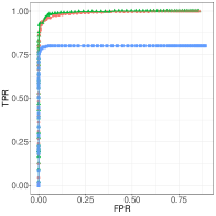
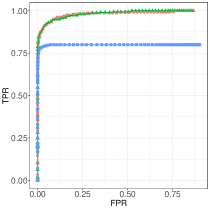
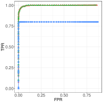
In this section, we assess the performance of our methodology in the case where Y1,,Ynsubscript𝑌1subscript𝑌𝑛Y_{1},\dots,Y_{n} satisfy the model defined by (1), (2) and (3) for n=1000𝑛1000n=1000, q{1,2,3}𝑞123q\in\{1,2,3\} and p=100𝑝100p=100. We shall moreover assume that the sparsity in the βisuperscriptsubscript𝛽𝑖\beta_{i}^{\star} is very high, namely all the βisuperscriptsubscript𝛽𝑖\beta_{i}^{\star} are assumed to be equal to zero except for five of them which are equal to 1.739, 0.387, 0.295, -0.644 and -0.135. The corresponding results are displayed in Figures 4, 5 and 6.
Refer to caption
Refer to caption
Figure 4. ROC curves for recovering the support of 𝜷superscript𝜷\boldsymbol{\beta}^{\star} in Model (2) with q=1𝑞1q=1 (left) and boxplot for the estimation of γ1superscriptsubscript𝛾1{\gamma_{1}}^{\star} in the same model (right). The ROC curve when γ1superscriptsubscript𝛾1{\gamma_{1}}^{\star} is known (resp. unknown) is in red (resp. green) and in the model where γ1=0superscriptsubscript𝛾10{\gamma_{1}}^{\star}=0 in blue. The horizontal lines correspond to the true values of the parameters.
Refer to caption
Refer to caption
Refer to caption
Figure 5. ROC curves for recovering the support of 𝜷superscript𝜷\boldsymbol{\beta}^{\star} in Model (2) with q=2𝑞2q=2 (left), boxplots for the estimation of γ1superscriptsubscript𝛾1{\gamma_{1}}^{\star} (middle) and γ2superscriptsubscript𝛾2{\gamma_{2}}^{\star} (right) in the same model. The ROC curve when γ1superscriptsubscript𝛾1{\gamma_{1}}^{\star} and γ2superscriptsubscript𝛾2{\gamma_{2}}^{\star} are known (resp. unknown) is in red (resp. green) and in the model where γ1=γ2=0superscriptsubscript𝛾1superscriptsubscript𝛾20{\gamma_{1}}^{\star}={\gamma_{2}}^{\star}=0 in blue. The horizontal lines correspond to the true values of the parameters.
Refer to caption
Refer to caption
Refer to caption
Refer to caption
Figure 6. ROC curves for recovering the support of 𝜷superscript𝜷\boldsymbol{\beta}^{\star} in Model (2) with q=3𝑞3q=3 (top left), boxplots for the estimation of γ1superscriptsubscript𝛾1{\gamma_{1}}^{\star} (top right), γ2superscriptsubscript𝛾2{\gamma_{2}}^{\star} (bottom left) and γ3superscriptsubscript𝛾3{\gamma_{3}}^{\star} (bottom right) in the same model. The ROC curve when γ1superscriptsubscript𝛾1{\gamma_{1}}^{\star}, γ2superscriptsubscript𝛾2{\gamma_{2}}^{\star} and γ3superscriptsubscript𝛾3{\gamma_{3}}^{\star} are known (resp. unknown) is in red (resp. green) and in the model where γ1=γ2=γ3=0superscriptsubscript𝛾1superscriptsubscript𝛾2superscriptsubscript𝛾30{\gamma_{1}}^{\star}={\gamma_{2}}^{\star}={\gamma_{3}}^{\star}=0 in blue. The horizontal lines correspond to the true values of the parameters.

The ROC curves of Figures 4, 5 and 6 display the True Positive Rate (TPR) with respect to the False Positive Rate (FPR). On the one hand, we can see from these figures that the performance of our methodology when 𝜸superscript𝜸\boldsymbol{\gamma}^{\star} is known is on a par with the one of our methodology when 𝜸superscript𝜸\boldsymbol{\gamma}^{\star} is unknown. On the other hand, our methodology outperforms the variable selection approach described in Friedman et al. (2010) which assumes that the observations are the realizations of a Poisson distribution but does not take into account the dependence between the observations.

We can also observe from these figures that the performance of our methodology is not altered by the underestimation of 𝜸superscript𝜸\boldsymbol{\gamma}^{\star} in the different situations: q=1𝑞1q=1, 2 or 3.

3.1.3. Choice of λ𝜆\lambda

In order to improve our methodology, we propose hereafter a strategy for tuning the parameter λ𝜆\lambda appearing in (11).

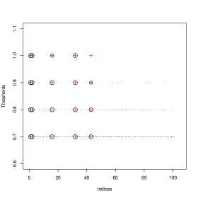
We first take the smallest λ𝜆\lambda provided by the glmnet package for computing (11). This λ𝜆\lambda denoted λminsubscript𝜆min\lambda_{\textrm{min}} is then used in the stability selection procedure proposed by Meinshausen and Bühlmann (2010) which guarantees the robustness of the selected variables. This latter approach can be described as follows. The vector 𝒴𝒴\mathcal{Y} defined in (22) is randomly split into several subsamples of size (p+1)/2𝑝12(p+1)/2, which corresponds to the half of the length of 𝒴𝒴\mathcal{Y}. For each subsample, the LASSO criterion is applied with λ=λmin𝜆subscript𝜆min\lambda=\lambda_{\textrm{min}} and the indices i𝑖i of the non null β^isubscript^𝛽𝑖\widehat{\beta}_{i} are stored. Then, for a given threshold, we keep in the final set of selected variables only the variables appearing a number of times larger than this threshold. In practice, we generated 100010001000 subsamples of 𝒴𝒴\mathcal{Y}.

Figure 7 displays the results obtained when applying this strategy to observations Y1,,Ynsubscript𝑌1subscript𝑌𝑛Y_{1},\dots,Y_{n} satisfying the model defined by (1), (2) and (3) for n=1000𝑛1000n=1000, q=1𝑞1q=1, p=100𝑝100p=100 and when only five coefficients βisuperscriptsubscript𝛽𝑖\beta_{i}^{\star} are not null. We can see from this figure that the positions of the non null coefficients are well retrieved for most of the thresholds and that the number of false positive is higher when the threshold is too low. Based on this figure, taking a threshold equal to 0.9 seems to achieve an interesting trade-off between false and true positives.
Refer to caption
Figure 7. Means of the selection frequencies of the indices of the final estimator of 𝜷superscript𝜷\boldsymbol{\beta}^{\star} for different thresholds: 0.7, 0.8, 0.9 and 1 and based on 100 replications. The larger the size of circles the larger the frequency of considering the corresponding coefficients as non null. The positions of the non null values of 𝜷superscript𝜷\boldsymbol{\beta}^{\star} are displayed with red crosses.

This choice is also confirmed by the results of Figure 8 which gives the means of selection frequencies for each position.

Refer to captionRefer to captionRefer to captionRefer to caption
Figure 8. Means of the selection frequencies of the indices of the final estimator of 𝜷superscript𝜷\boldsymbol{\beta}^{\star} based on 100 replications for different thresholds: 0.7 (top left), 0.8 (top right), 0.9 (bottom left) and 1 (bottom right). The positions of the non null values of 𝜷superscript𝜷\boldsymbol{\beta}^{\star} are displayed with red plain circles.

3.2. Numerical performance

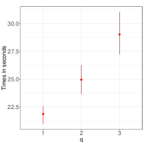
Figure 9 displays the means and standard errors of the computational times for our variable selection method. We can see from this figure that it takes only around 30 seconds to process observations Y1,,Ynsubscript𝑌1subscript𝑌𝑛Y_{1},\dots,Y_{n} satisfying (1), (2) and (3) when n=1000𝑛1000n=1000, p=100𝑝100p=100, q=3𝑞3q=3 and when the number of replications used in the stability selection step described in Section 3.1.3 is equal to 1000.
Refer to caption
Figure 9. Means and standard errors of the computational times in seconds for our variable selection approach in the case where n=1000𝑛1000n=1000, p=100𝑝100p=100, q=1𝑞1q=1, 2 and 3.

4. Proofs

4.1. Computation of the first and second derivatives of Wtsubscript𝑊𝑡W_{t} defined in (5)

The computations given below are similar to those provided in Davis et al. (2005) but are specific to the parametrization 𝜹=(𝜷,𝜸)𝜹superscript𝜷superscript𝜸\boldsymbol{\delta}=(\boldsymbol{\beta}^{\prime},\boldsymbol{\gamma}^{\prime}) considered in this paper.

4.1.1. Computation of the first derivatives of Wtsubscript𝑊𝑡W_{t}

By the definition of Wtsubscript𝑊𝑡W_{t} given in (5), we get

Wt𝜹(𝜹)=𝜷xt𝜹+Zt𝜹(𝜹),subscript𝑊𝑡𝜹𝜹superscript𝜷subscript𝑥𝑡𝜹subscript𝑍𝑡𝜹𝜹\frac{\partial W_{t}}{\partial\boldsymbol{\delta}}(\boldsymbol{\delta})=\frac{\partial\boldsymbol{\beta}^{\prime}x_{t}}{\partial\boldsymbol{\delta}}+\frac{\partial Z_{t}}{\partial\boldsymbol{\delta}}(\boldsymbol{\delta}),

where 𝜷𝜷\boldsymbol{\beta}, xtsubscript𝑥𝑡x_{t} and Ztsubscript𝑍𝑡Z_{t} are defined in (5). More precisely, for all k{0,,p}𝑘0𝑝k\in\{0,\dots,p\}, {1,,q}1𝑞\ell\in\{1,\dots,q\} and t{1,,n}𝑡1𝑛t\in\{1,\dots,n\}, by (6),

Wtβksubscript𝑊𝑡subscript𝛽𝑘\displaystyle\frac{\partial W_{t}}{\partial\beta_{k}} =xt,k+Ztβk=xt,k+j=1q(t1)γjEtjβkabsentsubscript𝑥𝑡𝑘subscript𝑍𝑡subscript𝛽𝑘subscript𝑥𝑡𝑘superscriptsubscript𝑗1𝑞𝑡1subscript𝛾𝑗subscript𝐸𝑡𝑗subscript𝛽𝑘\displaystyle=x_{t,k}+\frac{\partial Z_{t}}{\partial\beta_{k}}=x_{t,k}+\sum_{j=1}^{q\wedge(t-1)}\gamma_{j}\frac{\partial E_{t-j}}{\partial\beta_{k}}
(18) =xt,kj=1q(t1)γjYtjWtjβkexp(Wtj)=xt,kj=1q(t1)γj(1+Etj)Wtjβk,absentsubscript𝑥𝑡𝑘superscriptsubscript𝑗1𝑞𝑡1subscript𝛾𝑗subscript𝑌𝑡𝑗subscript𝑊𝑡𝑗subscript𝛽𝑘subscript𝑊𝑡𝑗subscript𝑥𝑡𝑘superscriptsubscript𝑗1𝑞𝑡1subscript𝛾𝑗1subscript𝐸𝑡𝑗subscript𝑊𝑡𝑗subscript𝛽𝑘\displaystyle=x_{t,k}-\sum_{j=1}^{q\wedge(t-1)}\gamma_{j}Y_{t-j}\frac{\partial W_{t-j}}{\partial\beta_{k}}\exp(-W_{t-j})=x_{t,k}-\sum_{j=1}^{q\wedge(t-1)}\gamma_{j}(1+E_{t-j})\frac{\partial W_{t-j}}{\partial\beta_{k}},
Wtγsubscript𝑊𝑡subscript𝛾\displaystyle\frac{\partial W_{t}}{\partial\gamma_{\ell}} =Et+j=1q(t1)γjEtjγabsentsubscript𝐸𝑡superscriptsubscript𝑗1𝑞𝑡1subscript𝛾𝑗subscript𝐸𝑡𝑗subscript𝛾\displaystyle=E_{t-\ell}+\sum_{j=1}^{q\wedge(t-1)}\gamma_{j}\frac{\partial E_{t-j}}{\partial\gamma_{\ell}}
(19) =Etj=1q(t1)γjYtjWtjγexp(Wtj)=Etj=1q(t1)γj(1+Etj)Wtjγ,absentsubscript𝐸𝑡superscriptsubscript𝑗1𝑞𝑡1subscript𝛾𝑗subscript𝑌𝑡𝑗subscript𝑊𝑡𝑗subscript𝛾subscript𝑊𝑡𝑗subscript𝐸𝑡superscriptsubscript𝑗1𝑞𝑡1subscript𝛾𝑗1subscript𝐸𝑡𝑗subscript𝑊𝑡𝑗subscript𝛾\displaystyle=E_{t-\ell}-\sum_{j=1}^{q\wedge(t-1)}\gamma_{j}Y_{t-j}\frac{\partial W_{t-j}}{\partial\gamma_{\ell}}\exp(-W_{t-j})=E_{t-\ell}-\sum_{j=1}^{q\wedge(t-1)}\gamma_{j}(1+E_{t-j})\frac{\partial W_{t-j}}{\partial\gamma_{\ell}},

where we used that Et=0,t0formulae-sequencesubscript𝐸𝑡0for-all𝑡0E_{t}=0,\;\forall t\leq 0.

The first derivatives of Wtsubscript𝑊𝑡W_{t} are thus obtained from the following recursive expressions. For all k{0,,p}𝑘0𝑝k\in\{0,\dots,p\}

W1βksubscript𝑊1subscript𝛽𝑘\displaystyle\frac{\partial W_{1}}{\partial\beta_{k}} =x1,k,absentsubscript𝑥1𝑘\displaystyle=x_{1,k},
W2βksubscript𝑊2subscript𝛽𝑘\displaystyle\frac{\partial W_{2}}{\partial\beta_{k}} =x2,kγ1(1+E1)W1βk,absentsubscript𝑥2𝑘subscript𝛾11subscript𝐸1subscript𝑊1subscript𝛽𝑘\displaystyle=x_{2,k}-\gamma_{1}(1+E_{1})\frac{\partial W_{1}}{\partial\beta_{k}},

where

(20) W1=𝜷x1 and E1=Y1exp(W1)1.subscript𝑊1superscript𝜷subscript𝑥1 and subscript𝐸1subscript𝑌1subscript𝑊11W_{1}=\boldsymbol{\beta}^{\prime}x_{1}\textrm{ and }E_{1}=Y_{1}\exp(-W_{1})-1.

Moreover,

W3βk=x3,kγ1(1+E2)W2βkγ2(1+E1)W1βk,subscript𝑊3subscript𝛽𝑘subscript𝑥3𝑘subscript𝛾11subscript𝐸2subscript𝑊2subscript𝛽𝑘subscript𝛾21subscript𝐸1subscript𝑊1subscript𝛽𝑘\frac{\partial W_{3}}{\partial\beta_{k}}=x_{3,k}-\gamma_{1}(1+E_{2})\frac{\partial W_{2}}{\partial\beta_{k}}-\gamma_{2}(1+E_{1})\frac{\partial W_{1}}{\partial\beta_{k}},

where

(21) W2=𝜷x2+γ1E1,E2=Y2exp(W2)1,formulae-sequencesubscript𝑊2superscript𝜷subscript𝑥2subscript𝛾1subscript𝐸1subscript𝐸2subscript𝑌2subscript𝑊21W_{2}=\boldsymbol{\beta}^{\prime}x_{2}+\gamma_{1}E_{1},\;E_{2}=Y_{2}\exp(-W_{2})-1,

and so on. In the same way, for all {1,,q}1𝑞\ell\in\{1,\dots,q\}

W1γsubscript𝑊1subscript𝛾\displaystyle\frac{\partial W_{1}}{\partial\gamma_{\ell}} =0,absent0\displaystyle=0,
W2γsubscript𝑊2subscript𝛾\displaystyle\frac{\partial W_{2}}{\partial\gamma_{\ell}} =E2,absentsubscript𝐸2\displaystyle=E_{2-\ell},
W3γsubscript𝑊3subscript𝛾\displaystyle\frac{\partial W_{3}}{\partial\gamma_{\ell}} =E3γ1(1+E2)W2γabsentsubscript𝐸3subscript𝛾11subscript𝐸2subscript𝑊2subscript𝛾\displaystyle=E_{3-\ell}-\gamma_{1}(1+E_{2})\frac{\partial W_{2}}{\partial\gamma_{\ell}}

and so on, where Et=0,t0formulae-sequencesubscript𝐸𝑡0for-all𝑡0E_{t}=0,\;\forall t\leq 0 and E1subscript𝐸1E_{1}, E2subscript𝐸2E_{2} are defined in (20) and (21), respectively.

4.1.2. Computation of the second derivatives of Wtsubscript𝑊𝑡W_{t}

Using (4.1.1) and (19), we get that for all j,k{0,,p}𝑗𝑘0𝑝j,k\in\{0,\dots,p\}, ,m{1,,q}𝑚1𝑞\ell,m\in\{1,\dots,q\} and t{1,,n}𝑡1𝑛t\in\{1,\dots,n\},

2Wtβjβksuperscript2subscript𝑊𝑡subscript𝛽𝑗subscript𝛽𝑘\displaystyle\frac{\partial^{2}W_{t}}{\partial\beta_{j}\partial\beta_{k}} =i=1q(t1)γi(1+Eti)2Wtiβjβki=1q(t1)γiEtiβjWtiβkabsentsuperscriptsubscript𝑖1𝑞𝑡1subscript𝛾𝑖1subscript𝐸𝑡𝑖superscript2subscript𝑊𝑡𝑖subscript𝛽𝑗subscript𝛽𝑘superscriptsubscript𝑖1𝑞𝑡1subscript𝛾𝑖subscript𝐸𝑡𝑖subscript𝛽𝑗subscript𝑊𝑡𝑖subscript𝛽𝑘\displaystyle=-\sum_{i=1}^{q\wedge(t-1)}\gamma_{i}(1+E_{t-i})\frac{\partial^{2}W_{t-i}}{\partial\beta_{j}\partial\beta_{k}}-\sum_{i=1}^{q\wedge(t-1)}\gamma_{i}\frac{\partial E_{t-i}}{\partial\beta_{j}}\frac{\partial W_{t-i}}{\partial\beta_{k}}
=i=1q(t1)γi(1+Eti)2Wtiβjβk+i=1q(t1)γi(1+Eti)WtiβjWtiβk,absentsuperscriptsubscript𝑖1𝑞𝑡1subscript𝛾𝑖1subscript𝐸𝑡𝑖superscript2subscript𝑊𝑡𝑖subscript𝛽𝑗subscript𝛽𝑘superscriptsubscript𝑖1𝑞𝑡1subscript𝛾𝑖1subscript𝐸𝑡𝑖subscript𝑊𝑡𝑖subscript𝛽𝑗subscript𝑊𝑡𝑖subscript𝛽𝑘\displaystyle=-\sum_{i=1}^{q\wedge(t-1)}\gamma_{i}(1+E_{t-i})\frac{\partial^{2}W_{t-i}}{\partial\beta_{j}\partial\beta_{k}}+\sum_{i=1}^{q\wedge(t-1)}\gamma_{i}(1+E_{t-i})\frac{\partial W_{t-i}}{\partial\beta_{j}}\frac{\partial W_{t-i}}{\partial\beta_{k}},
2Wtβkγsuperscript2subscript𝑊𝑡subscript𝛽𝑘subscript𝛾\displaystyle\frac{\partial^{2}W_{t}}{\partial\beta_{k}\partial\gamma_{\ell}} =(1+Et)Wtβki=1q(t1)γi{WtiβkEtiγ+(1+Eti)2Wtiβkγ}absent1subscript𝐸𝑡subscript𝑊𝑡subscript𝛽𝑘superscriptsubscript𝑖1𝑞𝑡1subscript𝛾𝑖subscript𝑊𝑡𝑖subscript𝛽𝑘subscript𝐸𝑡𝑖subscript𝛾1subscript𝐸𝑡𝑖superscript2subscript𝑊𝑡𝑖subscript𝛽𝑘subscript𝛾\displaystyle=-(1+E_{t-\ell})\frac{\partial W_{t-\ell}}{\partial\beta_{k}}-\sum_{i=1}^{q\wedge(t-1)}\gamma_{i}\left\{\frac{\partial W_{t-i}}{\partial\beta_{k}}\frac{\partial E_{t-i}}{\partial\gamma_{\ell}}+(1+E_{t-i})\frac{\partial^{2}W_{t-i}}{\partial\beta_{k}\partial\gamma_{\ell}}\right\}
=(1+Et)Wtβki=1q(t1)γi{(1+Eti)WtiβkWtiγ+(1+Eti)2Wtiβkγ},absent1subscript𝐸𝑡subscript𝑊𝑡subscript𝛽𝑘superscriptsubscript𝑖1𝑞𝑡1subscript𝛾𝑖1subscript𝐸𝑡𝑖subscript𝑊𝑡𝑖subscript𝛽𝑘subscript𝑊𝑡𝑖subscript𝛾1subscript𝐸𝑡𝑖superscript2subscript𝑊𝑡𝑖subscript𝛽𝑘subscript𝛾\displaystyle=-(1+E_{t-\ell})\frac{\partial W_{t-\ell}}{\partial\beta_{k}}-\sum_{i=1}^{q\wedge(t-1)}\gamma_{i}\left\{-(1+E_{t-i})\frac{\partial W_{t-i}}{\partial\beta_{k}}\frac{\partial W_{t-i}}{\partial\gamma_{\ell}}+(1+E_{t-i})\frac{\partial^{2}W_{t-i}}{\partial\beta_{k}\partial\gamma_{\ell}}\right\},
2Wtγγmsuperscript2subscript𝑊𝑡subscript𝛾subscript𝛾𝑚\displaystyle\frac{\partial^{2}W_{t}}{\partial\gamma_{\ell}\partial\gamma_{m}} =Etγm(1+Etm)Wtmγi=1q(t1)γi{WtiγEtiγm+(1+Eti)2Wtiγγm}absentsubscript𝐸𝑡subscript𝛾𝑚1subscript𝐸𝑡𝑚subscript𝑊𝑡𝑚subscript𝛾superscriptsubscript𝑖1𝑞𝑡1subscript𝛾𝑖subscript𝑊𝑡𝑖subscript𝛾subscript𝐸𝑡𝑖subscript𝛾𝑚1subscript𝐸𝑡𝑖superscript2subscript𝑊𝑡𝑖subscript𝛾subscript𝛾𝑚\displaystyle=\frac{\partial E_{t-\ell}}{\partial\gamma_{m}}-(1+E_{t-m})\frac{\partial W_{t-m}}{\partial\gamma_{\ell}}-\sum_{i=1}^{q\wedge(t-1)}\gamma_{i}\left\{\frac{\partial W_{t-i}}{\partial\gamma_{\ell}}\frac{\partial E_{t-i}}{\partial\gamma_{m}}+(1+E_{t-i})\frac{\partial^{2}W_{t-i}}{\partial\gamma_{\ell}\partial\gamma_{m}}\right\}
=(1+Et)Wtγm(1+Etm)Wtmγabsent1subscript𝐸𝑡subscript𝑊𝑡subscript𝛾𝑚1subscript𝐸𝑡𝑚subscript𝑊𝑡𝑚subscript𝛾\displaystyle=-(1+E_{t-\ell})\frac{\partial W_{t-\ell}}{\partial\gamma_{m}}-(1+E_{t-m})\frac{\partial W_{t-m}}{\partial\gamma_{\ell}}
i=1q(t1)γi{(1+Eti)WtiγWtiγm+(1+Eti)2Wtiγγm}.superscriptsubscript𝑖1𝑞𝑡1subscript𝛾𝑖1subscript𝐸𝑡𝑖subscript𝑊𝑡𝑖subscript𝛾subscript𝑊𝑡𝑖subscript𝛾𝑚1subscript𝐸𝑡𝑖superscript2subscript𝑊𝑡𝑖subscript𝛾subscript𝛾𝑚\displaystyle-\sum_{i=1}^{q\wedge(t-1)}\gamma_{i}\left\{-(1+E_{t-i})\frac{\partial W_{t-i}}{\partial\gamma_{\ell}}\frac{\partial W_{t-i}}{\partial\gamma_{m}}+(1+E_{t-i})\frac{\partial^{2}W_{t-i}}{\partial\gamma_{\ell}\partial\gamma_{m}}\right\}.

To compute the second derivatives of Wtsubscript𝑊𝑡W_{t}, we shall use the following recursive expressions for all j,k{0,,p}𝑗𝑘0𝑝j,k\in\{0,\dots,p\}

2W1βjβksuperscript2subscript𝑊1subscript𝛽𝑗subscript𝛽𝑘\displaystyle\frac{\partial^{2}W_{1}}{\partial\beta_{j}\partial\beta_{k}} =0,absent0\displaystyle=0,
2W2βjβksuperscript2subscript𝑊2subscript𝛽𝑗subscript𝛽𝑘\displaystyle\frac{\partial^{2}W_{2}}{\partial\beta_{j}\partial\beta_{k}} =γ1(1+E1)x1,jx1,k,absentsubscript𝛾11subscript𝐸1subscript𝑥1𝑗subscript𝑥1𝑘\displaystyle=\gamma_{1}(1+E_{1})x_{1,j}x_{1,k},

where E1subscript𝐸1E_{1} is defined in (20) and so on. Moreover, for all k{0,,p}𝑘0𝑝k\in\{0,\dots,p\} and {1,,q}1𝑞\ell\in\{1,\dots,q\}

2W1βkγsuperscript2subscript𝑊1subscript𝛽𝑘subscript𝛾\displaystyle\frac{\partial^{2}W_{1}}{\partial\beta_{k}\partial\gamma_{\ell}} =0,absent0\displaystyle=0,
2W2βkγsuperscript2subscript𝑊2subscript𝛽𝑘subscript𝛾\displaystyle\frac{\partial^{2}W_{2}}{\partial\beta_{k}\partial\gamma_{\ell}} =(1+E2)W2βk,absent1subscript𝐸2subscript𝑊2subscript𝛽𝑘\displaystyle=-(1+E_{2-\ell})\frac{\partial W_{2-\ell}}{\partial\beta_{k}},

where Et=0subscript𝐸𝑡0E_{t}=0 for all t0𝑡0t\leq 0 and the first derivatives of Wtsubscript𝑊𝑡W_{t} are computed in (4.1.1). Note also that

2W1γγmsuperscript2subscript𝑊1subscript𝛾subscript𝛾𝑚\displaystyle\frac{\partial^{2}W_{1}}{\partial\gamma_{\ell}\partial\gamma_{m}} =0,absent0\displaystyle=0,
2W2γγmsuperscript2subscript𝑊2subscript𝛾subscript𝛾𝑚\displaystyle\frac{\partial^{2}W_{2}}{\partial\gamma_{\ell}\partial\gamma_{m}} =0absent0\displaystyle=0

and so on.

4.2. Computational details for obtaining Criterion (11)

By (10),

L~(𝜷)=L~(𝜷~)+L𝜷(𝜷~,𝜸^)U(𝝂𝝂~)12(𝝂𝝂~)Λ(𝝂𝝂~),~𝐿𝜷~𝐿~𝜷𝐿𝜷~𝜷^𝜸𝑈𝝂~𝝂12superscript𝝂~𝝂Λ𝝂~𝝂\displaystyle\widetilde{L}(\boldsymbol{\beta})=\widetilde{L}(\widetilde{\boldsymbol{\beta}})+\frac{\partial L}{\partial\boldsymbol{\beta}}(\widetilde{\boldsymbol{\beta}},\widehat{\boldsymbol{\gamma}})U(\boldsymbol{\nu}-\widetilde{\boldsymbol{\nu}})-\frac{1}{2}(\boldsymbol{\nu}-\widetilde{\boldsymbol{\nu}})^{\prime}\Lambda(\boldsymbol{\nu}-\widetilde{\boldsymbol{\nu}}),

where 𝝂𝝂~=U(𝜷𝜷~)𝝂~𝝂superscript𝑈𝜷~𝜷\boldsymbol{\nu}-\widetilde{\boldsymbol{\nu}}=U^{\prime}(\boldsymbol{\beta}-\widetilde{\boldsymbol{\beta}}). Hence,

L~(𝜷)~𝐿𝜷\displaystyle\widetilde{L}(\boldsymbol{\beta}) =L~(𝜷~)+k=0p(L𝜷(𝜷~,𝜸^)U)k(νkν~k)12k=0pλk(νkν~k)2absent~𝐿~𝜷superscriptsubscript𝑘0𝑝subscript𝐿𝜷~𝜷^𝜸𝑈𝑘subscript𝜈𝑘subscript~𝜈𝑘12superscriptsubscript𝑘0𝑝subscript𝜆𝑘superscriptsubscript𝜈𝑘subscript~𝜈𝑘2\displaystyle=\widetilde{L}(\widetilde{\boldsymbol{\beta}})+\sum_{k=0}^{p}\left(\frac{\partial L}{\partial\boldsymbol{\beta}}(\widetilde{\boldsymbol{\beta}},\widehat{\boldsymbol{\gamma}})U\right)_{k}(\nu_{k}-\widetilde{\nu}_{k})-\frac{1}{2}\sum_{k=0}^{p}\lambda_{k}(\nu_{k}-\widetilde{\nu}_{k})^{2}
=L~(𝜷~)12k=0pλk(νkν~k1λk(L𝜷(𝜷~,𝜸^)U)k)2+k=0p12λk(L𝜷(𝜷~,𝜸^)U)k2,absent~𝐿~𝜷12superscriptsubscript𝑘0𝑝subscript𝜆𝑘superscriptsubscript𝜈𝑘subscript~𝜈𝑘1subscript𝜆𝑘subscript𝐿𝜷~𝜷^𝜸𝑈𝑘2superscriptsubscript𝑘0𝑝12subscript𝜆𝑘superscriptsubscript𝐿𝜷~𝜷^𝜸𝑈𝑘2\displaystyle=\widetilde{L}(\widetilde{\boldsymbol{\beta}})-\frac{1}{2}\sum_{k=0}^{p}\lambda_{k}\left(\nu_{k}-\widetilde{\nu}_{k}-\frac{1}{\lambda_{k}}\left(\frac{\partial L}{\partial\boldsymbol{\beta}}(\widetilde{\boldsymbol{\beta}},\widehat{\boldsymbol{\gamma}})U\right)_{k}\right)^{2}+\sum_{k=0}^{p}\frac{1}{2\lambda_{k}}\left(\frac{\partial L}{\partial\boldsymbol{\beta}}(\widetilde{\boldsymbol{\beta}},\widehat{\boldsymbol{\gamma}})U\right)_{k}^{2},

where the λksubscript𝜆𝑘\lambda_{k}’s are the diagonal terms of ΛΛ\Lambda.

Since the only term depending on 𝜷𝜷\boldsymbol{\beta} is the second one in the last expression of L~(𝜷)~𝐿𝜷\widetilde{L}(\boldsymbol{\beta}), we define L~Q(𝜷)subscript~𝐿𝑄𝜷\widetilde{L}_{Q}(\boldsymbol{\beta}) appearing in Criterion (11) as follows:

L~Q(𝜷)subscript~𝐿𝑄𝜷\displaystyle-\widetilde{L}_{Q}(\boldsymbol{\beta}) =\displaystyle= 12k=0pλk(νkν~k+1λk(L𝜷(𝜷~,𝜸^)U)k)212superscriptsubscript𝑘0𝑝subscript𝜆𝑘superscriptsubscript𝜈𝑘subscript~𝜈𝑘1subscript𝜆𝑘subscript𝐿𝜷~𝜷^𝜸𝑈𝑘2\displaystyle\frac{1}{2}\sum_{k=0}^{p}\lambda_{k}\left(\nu_{k}-\widetilde{\nu}_{k}+\frac{1}{\lambda_{k}}\left(\frac{\partial L}{\partial\boldsymbol{\beta}}(\widetilde{\boldsymbol{\beta}},\widehat{\boldsymbol{\gamma}})U\right)_{k}\right)^{2}
=\displaystyle= 12Λ1/2(𝝂𝝂~+Λ1(L𝜷(𝜷~,𝜸^)U))2212superscriptsubscriptnormsuperscriptΛ12𝝂~𝝂superscriptΛ1superscript𝐿𝜷~𝜷^𝜸𝑈22\displaystyle\frac{1}{2}\left\|\Lambda^{1/2}\left(\boldsymbol{\nu}-\widetilde{\boldsymbol{\nu}}+\Lambda^{-1}\left(\frac{\partial L}{\partial\boldsymbol{\beta}}(\widetilde{\boldsymbol{\beta}},\widehat{\boldsymbol{\gamma}})U\right)^{\prime}\right)\right\|_{2}^{2}
=\displaystyle= 12Λ1/2U(𝜷𝜷~)+Λ1/2U(L𝜷(𝜷~,𝜸^))2212superscriptsubscriptnormsuperscriptΛ12superscript𝑈𝜷~𝜷superscriptΛ12superscript𝑈superscript𝐿𝜷~𝜷^𝜸22\displaystyle\frac{1}{2}\left\|\Lambda^{1/2}U^{\prime}(\boldsymbol{\beta}-\widetilde{\boldsymbol{\beta}})+\Lambda^{-1/2}U^{\prime}\left(\frac{\partial L}{\partial\boldsymbol{\beta}}(\widetilde{\boldsymbol{\beta}},\widehat{\boldsymbol{\gamma}})\right)^{\prime}\right\|_{2}^{2}
=\displaystyle= 12Λ1/2U(𝜷~𝜷)Λ1/2U(L𝜷(𝜷~,𝜸^))2212superscriptsubscriptnormsuperscriptΛ12superscript𝑈~𝜷𝜷superscriptΛ12superscript𝑈superscript𝐿𝜷~𝜷^𝜸22\displaystyle\frac{1}{2}\left\|\Lambda^{1/2}U^{\prime}(\widetilde{\boldsymbol{\beta}}-\boldsymbol{\beta})-\Lambda^{-1/2}U^{\prime}\left(\frac{\partial L}{\partial\boldsymbol{\beta}}(\widetilde{\boldsymbol{\beta}},\widehat{\boldsymbol{\gamma}})\right)^{\prime}\right\|_{2}^{2}
=\displaystyle= 12𝒴𝒳𝜷22,12superscriptsubscriptnorm𝒴𝒳𝜷22\displaystyle\frac{1}{2}\|\mathcal{Y}-\mathcal{X}\boldsymbol{\beta}\|_{2}^{2},

where

(22) 𝒴=Λ1/2U𝜷~Λ1/2U(L𝜷(𝜷~,𝜸^)),𝒳=Λ1/2U.formulae-sequence𝒴superscriptΛ12superscript𝑈~𝜷superscriptΛ12superscript𝑈superscript𝐿𝜷~𝜷^𝜸𝒳superscriptΛ12superscript𝑈\mathcal{Y}=\Lambda^{1/2}U^{\prime}\widetilde{\boldsymbol{\beta}}-\Lambda^{-1/2}U^{\prime}\left(\frac{\partial L}{\partial\boldsymbol{\beta}}(\widetilde{\boldsymbol{\beta}},\widehat{\boldsymbol{\gamma}})\right)^{\prime},\;\mathcal{X}=\Lambda^{1/2}U^{\prime}.

4.3. Proofs of Propositions 1, 2 and 3 and of Lemma 1

This section contains the proofs of Propositions 1, 2 and 3.

4.3.1. Proof of Proposition 1

We first establish the following lemma for proving Proposition 1.

Lemma 1.

(Wt)superscriptsubscript𝑊𝑡(W_{t}^{\star}) is an aperiodic Markov process satisfying Doeblin’s condition.

Proof of Lemma 1.

By (14) and (3), we observe that:

(23) Wt=(β0γ1)+γ1Yt1exp(Wt1).superscriptsubscript𝑊𝑡superscriptsubscript𝛽0superscriptsubscript𝛾1superscriptsubscript𝛾1subscript𝑌𝑡1superscriptsubscript𝑊𝑡1W_{t}^{\star}=(\beta_{0}^{\star}-\gamma_{1}^{\star})+\gamma_{1}^{\star}Y_{t-1}\exp(-W_{t-1}^{\star}).

Thus, t2=t1W:=σ(Ws,st1)subscript𝑡2superscriptsubscript𝑡1superscript𝑊assign𝜎subscript𝑊𝑠𝑠𝑡1\mathcal{F}_{t-2}=\mathcal{F}_{t-1}^{W^{\star}}:=\sigma(W_{s},s\leq t-1). By (1), the distribution of Yt1subscript𝑌𝑡1Y_{t-1} conditionally to t2subscript𝑡2\mathcal{F}_{t-2} is 𝒫(exp(Wt1))𝒫superscriptsubscript𝑊𝑡1\mathcal{P}(\exp(W_{t-1}^{\star})). Hence, the distribution of Wtsuperscriptsubscript𝑊𝑡W_{t}^{\star} conditionally to t1Wsuperscriptsubscript𝑡1superscript𝑊\mathcal{F}_{t-1}^{W^{\star}} is the same as distribution of Wtsuperscriptsubscript𝑊𝑡W_{t}^{\star} conditionally to Wt1superscriptsubscript𝑊𝑡1W_{t-1}^{\star}, which means that (Wt)superscriptsubscript𝑊𝑡(W_{t}^{\star}) has the Markov property.

Let us now prove that (Wt)superscriptsubscript𝑊𝑡(W_{t}^{\star}) is strongly aperiodic which implies that it is aperiodic.

(Wt=β0γ1|Wt1=β0γ1)=(Yt1=0|Wt1=β0γ1)=exp(exp(β0γ1))>0,subscriptsuperscript𝑊𝑡superscriptsubscript𝛽0conditionalsuperscriptsubscript𝛾1subscriptsuperscript𝑊𝑡1superscriptsubscript𝛽0superscriptsubscript𝛾1subscript𝑌𝑡1conditional0subscriptsuperscript𝑊𝑡1superscriptsubscript𝛽0superscriptsubscript𝛾1superscriptsubscript𝛽0superscriptsubscript𝛾10\mathbb{P}(W^{\star}_{t}=\beta_{0}^{\star}-\gamma_{1}^{\star}|W^{\star}_{t-1}=\beta_{0}^{\star}-\gamma_{1}^{\star})=\mathbb{P}(Y_{t-1}=0|W^{\star}_{t-1}=\beta_{0}^{\star}-\gamma_{1}^{\star})=\exp(-\exp(\beta_{0}^{\star}-\gamma_{1}^{\star}))>0,

where the first equality comes from (23) and the last equality comes from (1) since t2=t1Wsubscript𝑡2superscriptsubscript𝑡1superscript𝑊\mathcal{F}_{t-2}=\mathcal{F}_{t-1}^{W^{\star}}.

To prove that (Wt)superscriptsubscript𝑊𝑡(W_{t}^{\star}) satisfies Doeblin’s condition namely that there exists a probability measure ν𝜈\nu with the property that, for some m1𝑚1m\geq 1, ε>0𝜀0\varepsilon>0 and δ>0𝛿0\delta>0,

(24) ν(B)>ε(Wt+m1B,Wt+m2B,Wt+1B,WtB|Wt1=x)δ,𝜈𝐵𝜀formulae-sequencesubscript𝑊𝑡𝑚1𝐵formulae-sequencesubscript𝑊𝑡𝑚2𝐵formulae-sequencesubscript𝑊𝑡1𝐵subscript𝑊𝑡conditional𝐵subscript𝑊𝑡1𝑥𝛿\nu(B)>\varepsilon\Longrightarrow\mathbb{P}(W_{t+m-1}\in B,W_{t+m-2}\in B\dots,W_{t+1}\in B,W_{t}\in B|W_{t-1}=x)\geq\delta,

for all x𝑥x in the state space X𝑋X of Wtsuperscriptsubscript𝑊𝑡W_{t}^{\star} and B𝐵B in the Borel sets of X𝑋X, we refer the reader to the proof of Proposition 2 in Davis et al. (2003).

Proof of Proposition 1.

For proving Proposition 1, we shall use Theorems 1.3.3 and 1.3.5 of Taniguchi and Kakizawa (2012). In order to apply these theorems it is enough to prove that (Wt)superscriptsubscript𝑊𝑡(W_{t}^{\star}) is a strictly stationary and ergodic process since YtWt(β0,γ1)exp(Wt(β0,γ1))subscript𝑌𝑡subscript𝑊𝑡superscriptsubscript𝛽0subscript𝛾1subscript𝑊𝑡superscriptsubscript𝛽0subscript𝛾1Y_{t}W_{t}(\beta_{0}^{\star},\gamma_{1})-\exp(W_{t}(\beta_{0}^{\star},\gamma_{1})) is a measurable function of Wt+1,Wt,,W2superscriptsubscript𝑊𝑡1superscriptsubscript𝑊𝑡superscriptsubscript𝑊2W_{t+1}^{\star},W_{t}^{\star},\dots,W_{2}^{\star}. Note that the latter fact comes from (14) and (3) for Ytsubscript𝑌𝑡Y_{t} and from (5) with q=1𝑞1q=1 and p=0𝑝0p=0 for Wtsubscript𝑊𝑡W_{t}.

In order to prove that (Wt)superscriptsubscript𝑊𝑡(W_{t}^{\star}) is a strictly stationary and ergodic process, we have first to prove that (Wt)superscriptsubscript𝑊𝑡(W_{t}^{\star}) is an aperiodic Markov process satisfying Doeblin’s condition, see Lemma 1.

The statement of Lemma 1 corresponds to Assertion (iv) of Theorem 16.0.2 of Meyn and Tweedie (1993) which is equivalent to Assertion (i) of this theorem, and implies that (Wt)superscriptsubscript𝑊𝑡(W_{t}^{\star}) is uniformly ergodic.

Hence, by Definition (16.6) of uniform ergodicity given in Meyn and Tweedie (1993), there exists a unique stationary invariant measure for (Wt)superscriptsubscript𝑊𝑡(W_{t}^{\star}), see also the paragraph below Equation (1.3) of Sandrić (2017) for an additional justification. Combining that existence of a unique stationary invariant measure for (Wt)superscriptsubscript𝑊𝑡(W_{t}^{\star}) with the following arguments shows that (Wt)superscriptsubscript𝑊𝑡(W_{t}^{\star}) is a strictly stationary process and also an ergodic Markov process.

By Theorem 3.6.3, Corollary 3.6.1 and Definition 3.6.6 of Stout (1974), if the process (Wt)superscriptsubscript𝑊𝑡(W_{t}^{\star}) is started with its unique stationary invariant distribution, (Wt)superscriptsubscript𝑊𝑡(W_{t}^{\star}) is a strictly stationary process.

By Definition 3.6.8 of Stout (1974), the existence of a unique stationary invariant measure for (Wt)superscriptsubscript𝑊𝑡(W_{t}^{\star}) means that (Wt)superscriptsubscript𝑊𝑡(W_{t}^{\star}) is an ergodic Markov process, see also the paragraph below (b) (Sandrić, 2017, p. 717).

Finally, by Theorem 3.6.5 of Stout (1974), since (Wt)superscriptsubscript𝑊𝑡(W_{t}^{\star}) is an ergodic Markov process and a strictly stationary process, (Wt)superscriptsubscript𝑊𝑡(W_{t}^{\star}) is an ergodic and strictly stationary process in the sense of the assumption of Theorem 1.3.5 of Taniguchi and Kakizawa (2012). ∎

4.3.2. Proof of Proposition 2

Note that for all γ1subscript𝛾1\gamma_{1},

(γ1)subscript𝛾1\displaystyle\mathcal{L}(\gamma_{1}) =𝔼[Y3W3(β0,γ1)exp(W3(β0,γ1))]=𝔼[𝔼[Y3W3(β0,γ1)exp(W3(β0,γ1))|2]]absent𝔼delimited-[]subscript𝑌3subscript𝑊3superscriptsubscript𝛽0subscript𝛾1subscript𝑊3superscriptsubscript𝛽0subscript𝛾1𝔼delimited-[]𝔼delimited-[]subscript𝑌3subscript𝑊3superscriptsubscript𝛽0subscript𝛾1conditionalsubscript𝑊3superscriptsubscript𝛽0subscript𝛾1subscript2\displaystyle=\mathbb{E}\left[Y_{3}W_{3}(\beta_{0}^{\star},\gamma_{1})-\exp(W_{3}(\beta_{0}^{\star},\gamma_{1}))\right]=\mathbb{E}\left[\mathbb{E}\left[Y_{3}W_{3}(\beta_{0}^{\star},\gamma_{1})-\exp(W_{3}(\beta_{0}^{\star},\gamma_{1}))|\mathcal{F}_{2}\right]\right]
=𝔼[exp(W3)W3(β0,γ1)exp(W3(β0,γ1))]absent𝔼delimited-[]superscriptsubscript𝑊3subscript𝑊3superscriptsubscript𝛽0subscript𝛾1subscript𝑊3superscriptsubscript𝛽0subscript𝛾1\displaystyle=\mathbb{E}\left[\exp(W_{3}^{\star})W_{3}(\beta_{0}^{\star},\gamma_{1})-\exp(W_{3}(\beta_{0}^{\star},\gamma_{1}))\right]
=𝔼[exp(W3)(W3(β0,γ1)W3+W3exp(W3(β0,γ1)W3))]absent𝔼delimited-[]superscriptsubscript𝑊3subscript𝑊3superscriptsubscript𝛽0subscript𝛾1superscriptsubscript𝑊3superscriptsubscript𝑊3subscript𝑊3superscriptsubscript𝛽0subscript𝛾1superscriptsubscript𝑊3\displaystyle=\mathbb{E}\left[\exp(W_{3}^{\star})\left(W_{3}(\beta_{0}^{\star},\gamma_{1})-W_{3}^{\star}+W_{3}^{\star}-\exp(W_{3}(\beta_{0}^{\star},\gamma_{1})-W_{3}^{\star})\right)\right]
𝔼[exp(W3)(W31)]=(γ1),absent𝔼delimited-[]superscriptsubscript𝑊3superscriptsubscript𝑊31superscriptsubscript𝛾1\displaystyle\leq\mathbb{E}\left[\exp(W_{3}^{\star})\left(W_{3}^{\star}-1\right)\right]=\mathcal{L}(\gamma_{1}^{\star}),

where the inequality comes from the following inequality xexp(x)1𝑥𝑥1x-\exp(x)\leq-1, for all x𝑥x\in\mathbb{R}. This inequality is an equality only when x=0𝑥0x=0 which means that γ1=γ1subscript𝛾1superscriptsubscript𝛾1\gamma_{1}=\gamma_{1}^{\star}.

4.3.3. Proof of Proposition 3

The proof of this proposition comes from Proposition 1 and the stochastic equicontinuity of n1L(β0,γ1)superscript𝑛1𝐿superscriptsubscript𝛽0subscript𝛾1n^{-1}L(\beta_{0}^{\star},\gamma_{1}). Thus, it is enough to prove that there exists a positive δ𝛿\delta such that

sup|γ1γ2|δ|L(β0,γ1)nL(β0,γ2)n|p0, as n tends to infinity.superscript𝑝subscriptsupremumsubscript𝛾1subscript𝛾2𝛿𝐿superscriptsubscript𝛽0subscript𝛾1𝑛𝐿superscriptsubscript𝛽0subscript𝛾2𝑛0 as n tends to infinity.\sup_{|\gamma_{1}-\gamma_{2}|\leq\delta}\left|\frac{L(\beta_{0}^{\star},\gamma_{1})}{n}-\frac{L(\beta_{0}^{\star},\gamma_{2})}{n}\right|\stackrel{{\scriptstyle p}}{{\longrightarrow}}0,\textrm{ as $n$ tends to infinity.}

Observe that, by (15),

|L(β0,γ1)nL(β0,γ2)n|𝐿superscriptsubscript𝛽0subscript𝛾1𝑛𝐿superscriptsubscript𝛽0subscript𝛾2𝑛\displaystyle\left|\frac{L(\beta_{0}^{\star},\gamma_{1})}{n}-\frac{L(\beta_{0}^{\star},\gamma_{2})}{n}\right| 1nt=1nYt|Wt(β0,γ1)Wt(β0,γ2)|absent1𝑛superscriptsubscript𝑡1𝑛subscript𝑌𝑡subscript𝑊𝑡superscriptsubscript𝛽0subscript𝛾1subscript𝑊𝑡superscriptsubscript𝛽0subscript𝛾2\displaystyle\leq\frac{1}{n}\sum_{t=1}^{n}Y_{t}\left|W_{t}(\beta_{0}^{\star},\gamma_{1})-W_{t}(\beta_{0}^{\star},\gamma_{2})\right|
+1nt=1n|exp(Wt(β0,γ1))exp(Wt(β0,γ2))|.1𝑛superscriptsubscript𝑡1𝑛subscript𝑊𝑡superscriptsubscript𝛽0subscript𝛾1subscript𝑊𝑡superscriptsubscript𝛽0subscript𝛾2\displaystyle+\frac{1}{n}\sum_{t=1}^{n}\left|\exp\left(W_{t}(\beta_{0}^{\star},\gamma_{1})\right)-\exp\left(W_{t}(\beta_{0}^{\star},\gamma_{2})\right)\right|.

Let us first focus on bounding the following expression for t2𝑡2t\geq 2 (since W1(β0,γ)=β0subscript𝑊1superscriptsubscript𝛽0𝛾superscriptsubscript𝛽0W_{1}(\beta_{0}^{\star},\gamma)=\beta_{0}^{\star}, for all γ𝛾\gamma). By (16)

|Wt(β0,γ1)Wt(β0,γ2)|=|Zt(γ1)Zt(γ2)|=|γ1Et1(γ1)γ2Et1(γ2)|subscript𝑊𝑡superscriptsubscript𝛽0subscript𝛾1subscript𝑊𝑡superscriptsubscript𝛽0subscript𝛾2subscript𝑍𝑡subscript𝛾1subscript𝑍𝑡subscript𝛾2subscript𝛾1subscript𝐸𝑡1subscript𝛾1subscript𝛾2subscript𝐸𝑡1subscript𝛾2\displaystyle\left|W_{t}(\beta_{0}^{\star},\gamma_{1})-W_{t}(\beta_{0}^{\star},\gamma_{2})\right|=\left|Z_{t}(\gamma_{1})-Z_{t}(\gamma_{2})\right|=\left|\gamma_{1}E_{t-1}(\gamma_{1})-\gamma_{2}E_{t-1}(\gamma_{2})\right|
=|γ1[Yt1exp(Wt1(β0,γ1))1]γ2[Yt1exp(Wt1(β0,γ2))1]|absentsubscript𝛾1delimited-[]subscript𝑌𝑡1subscript𝑊𝑡1superscriptsubscript𝛽0subscript𝛾11subscript𝛾2delimited-[]subscript𝑌𝑡1subscript𝑊𝑡1superscriptsubscript𝛽0subscript𝛾21\displaystyle=\left|\gamma_{1}\left[Y_{t-1}\exp(-W_{t-1}(\beta_{0}^{\star},\gamma_{1}))-1\right]-\gamma_{2}\left[Y_{t-1}\exp(-W_{t-1}(\beta_{0}^{\star},\gamma_{2}))-1\right]\right|
=|Yt1eβ0[γ1exp(Zt1(γ1))γ2exp(Zt1(γ2))]+γ2γ1|absentsubscript𝑌𝑡1superscriptesuperscriptsubscript𝛽0delimited-[]subscript𝛾1subscript𝑍𝑡1subscript𝛾1subscript𝛾2subscript𝑍𝑡1subscript𝛾2subscript𝛾2subscript𝛾1\displaystyle=\left|Y_{t-1}\textrm{e}^{-\beta_{0}^{\star}}\left[\gamma_{1}\exp(-Z_{t-1}(\gamma_{1}))-\gamma_{2}\exp(-Z_{t-1}(\gamma_{2}))\right]+\gamma_{2}-\gamma_{1}\right|
Yt1eβ0[|γ1γ2|exp(Zt1(γ1))+|γ2||exp(Zt1(γ1))exp(Zt1(γ2))|]+|γ2γ1|absentsubscript𝑌𝑡1superscriptesuperscriptsubscript𝛽0delimited-[]subscript𝛾1subscript𝛾2subscript𝑍𝑡1subscript𝛾1subscript𝛾2subscript𝑍𝑡1subscript𝛾1subscript𝑍𝑡1subscript𝛾2subscript𝛾2subscript𝛾1\displaystyle\leq Y_{t-1}\textrm{e}^{-\beta_{0}^{\star}}\left[\left|\gamma_{1}-\gamma_{2}\right|\exp(-Z_{t-1}(\gamma_{1}))+|\gamma_{2}|\left|\exp(-Z_{t-1}(\gamma_{1}))-\exp(-Z_{t-1}(\gamma_{2}))\right|\right]+\left|\gamma_{2}-\gamma_{1}\right|
Yt1eβ0|γ1γ2|exp(Zt1(γ1))absentsubscript𝑌𝑡1superscriptesuperscriptsubscript𝛽0subscript𝛾1subscript𝛾2subscript𝑍𝑡1subscript𝛾1\displaystyle\leq Y_{t-1}\textrm{e}^{-\beta_{0}^{\star}}\left|\gamma_{1}-\gamma_{2}\right|\exp(-Z_{t-1}(\gamma_{1}))
+Yt1eβ0|γ2|exp(Zt1(γ1))|Zt1(γ1)Zt1(γ2)|exp(|Zt1(γ1)Zt1(γ2)|)subscript𝑌𝑡1superscriptesuperscriptsubscript𝛽0subscript𝛾2subscript𝑍𝑡1subscript𝛾1subscript𝑍𝑡1subscript𝛾1subscript𝑍𝑡1subscript𝛾2subscript𝑍𝑡1subscript𝛾1subscript𝑍𝑡1subscript𝛾2\displaystyle+Y_{t-1}\textrm{e}^{-\beta_{0}^{\star}}|\gamma_{2}|\exp(-Z_{t-1}(\gamma_{1}))\left|Z_{t-1}(\gamma_{1})-Z_{t-1}(\gamma_{2})\right|\exp(|Z_{t-1}(\gamma_{1})-Z_{t-1}(\gamma_{2})|)
+|γ2γ1|,subscript𝛾2subscript𝛾1\displaystyle+\left|\gamma_{2}-\gamma_{1}\right|,

where we used in the last inequality that for all x𝑥x and y𝑦y in \mathbb{R},

(25) |exey|=ex|1eyx|ex|yx|e|yx|.superscripte𝑥superscripte𝑦superscripte𝑥1superscripte𝑦𝑥superscripte𝑥𝑦𝑥superscripte𝑦𝑥|\textrm{e}^{x}-\textrm{e}^{y}|=\textrm{e}^{x}|1-\textrm{e}^{y-x}|\leq\textrm{e}^{x}|y-x|\textrm{e}^{|y-x|}.

Observing that

(26) exp(Zt(γ1))=exp(γ1[Yt1eβ0exp(Zt1(γ1))1]),subscript𝑍𝑡subscript𝛾1subscript𝛾1delimited-[]subscript𝑌𝑡1superscriptesuperscriptsubscript𝛽0subscript𝑍𝑡1subscript𝛾11\exp(-Z_{t}(\gamma_{1}))=\exp\left(-\gamma_{1}\left[Y_{t-1}\textrm{e}^{-\beta_{0}^{\star}}\exp(-Z_{t-1}(\gamma_{1}))-1\right]\right),

and |Z2(γ1)Z2(γ2)|δ[Y1eβ0+1]subscript𝑍2subscript𝛾1subscript𝑍2subscript𝛾2𝛿delimited-[]subscript𝑌1superscriptesuperscriptsubscript𝛽01|Z_{2}(\gamma_{1})-Z_{2}(\gamma_{2})|\leq\delta[Y_{1}\textrm{e}^{-\beta_{0}^{\star}}+1] we get, for γ1subscript𝛾1\gamma_{1} and γ2subscript𝛾2\gamma_{2} such that |γ1γ2|δsubscript𝛾1subscript𝛾2𝛿|\gamma_{1}-\gamma_{2}|\leq\delta, that

(27) |Wt(β0,γ1)Wt(β0,γ2)|δF(Yt1,Yt2,,Y1),subscript𝑊𝑡superscriptsubscript𝛽0subscript𝛾1subscript𝑊𝑡superscriptsubscript𝛽0subscript𝛾2𝛿𝐹subscript𝑌𝑡1subscript𝑌𝑡2subscript𝑌1\left|W_{t}(\beta_{0}^{\star},\gamma_{1})-W_{t}(\beta_{0}^{\star},\gamma_{2})\right|\leq\delta\;F(Y_{t-1},Y_{t-2},\dots,Y_{1}),

where F𝐹F is a measurable function. By (25),

|exp(Wt(β0,γ1))exp(Wt(β0,γ2))|subscript𝑊𝑡superscriptsubscript𝛽0subscript𝛾1subscript𝑊𝑡superscriptsubscript𝛽0subscript𝛾2\displaystyle\left|\exp\left(W_{t}(\beta_{0}^{\star},\gamma_{1})\right)-\exp\left(W_{t}(\beta_{0}^{\star},\gamma_{2})\right)\right|
exp(Wt(β0,γ1))|Wt(β0,γ1)Wt(β0,γ2)|exp(|Wt(β0,γ1)Wt(β0,γ2)|)absentsubscript𝑊𝑡superscriptsubscript𝛽0subscript𝛾1subscript𝑊𝑡superscriptsubscript𝛽0subscript𝛾1subscript𝑊𝑡superscriptsubscript𝛽0subscript𝛾2subscript𝑊𝑡superscriptsubscript𝛽0subscript𝛾1subscript𝑊𝑡superscriptsubscript𝛽0subscript𝛾2\displaystyle\leq\exp\left(W_{t}(\beta_{0}^{\star},\gamma_{1})\right)\left|W_{t}(\beta_{0}^{\star},\gamma_{1})-W_{t}(\beta_{0}^{\star},\gamma_{2})\right|\exp\left(\left|W_{t}(\beta_{0}^{\star},\gamma_{1})-W_{t}(\beta_{0}^{\star},\gamma_{2})\right|\right)
δG(Yt1,Yt2,,Y1)absent𝛿𝐺subscript𝑌𝑡1subscript𝑌𝑡2subscript𝑌1\displaystyle\leq\delta G(Y_{t-1},Y_{t-2},\dots,Y_{1})

where the last inequality comes from (27), (26) and (16) and where G𝐺G is a measurable function. Thus, we get that

|L(β0,γ1)nL(β0,γ2)n|δnt=1nH(Yt,Yt1,,Y1),𝐿superscriptsubscript𝛽0subscript𝛾1𝑛𝐿superscriptsubscript𝛽0subscript𝛾2𝑛𝛿𝑛superscriptsubscript𝑡1𝑛𝐻subscript𝑌𝑡subscript𝑌𝑡1subscript𝑌1\left|\frac{L(\beta_{0}^{\star},\gamma_{1})}{n}-\frac{L(\beta_{0}^{\star},\gamma_{2})}{n}\right|\leq\frac{\delta}{n}\sum_{t=1}^{n}H(Y_{t},Y_{t-1},\dots,Y_{1}),

which gives the result by using similar arguments as those given in the proof of Proposition 1 namely that (Yt)subscript𝑌𝑡(Y_{t}) is strictly stationary and ergodic. By Theorem 1.3.3 of Taniguchi and Kakizawa (2012), H(Yt,Yt1,,Y1)𝐻subscript𝑌𝑡subscript𝑌𝑡1subscript𝑌1H(Y_{t},Y_{t-1},\dots,Y_{1}) is strictly stationary and ergodic since (Yt)subscript𝑌𝑡(Y_{t}) has these properties. Thus, 𝔼[|H(Yt,Yt1,,Y1)|]<𝔼delimited-[]𝐻subscript𝑌𝑡subscript𝑌𝑡1subscript𝑌1\mathbb{E}[|H(Y_{t},Y_{t-1},\dots,Y_{1})|]<\infty, which concludes the proof by Theorem 1.3.5 of Taniguchi and Kakizawa (2012).

References

  • Al-Osh and Alzaid (1988) Al-Osh, M. and A. A. Alzaid (1988). Integer-valued moving average (INMA) process. Statistical Papers 29(1), 281–300.
  • Brännäs and Quoreshi (2010) Brännäs, K. and A. M. M. S. Quoreshi (2010). Integer-valued moving average modelling of the number of transactions in stocks. Applied Financial Economics 20(18), 1429–1440.
  • Cox et al. (1981) Cox, D. R., G. Gudmundsson, G. Lindgren, L. Bondesson, E. Harsaae, P. Laake, K. Juselius, and S. L. Lauritzen (1981). Statistical analysis of time series: Some recent developments [with discussion and reply]. Scandinavian Journal of Statistics 8(2), 93–115.
  • Davis et al. (2003) Davis, R. A., W. T. M. Dunsmuir, and S. B. Streett (2003). Observation-driven models for Poisson counts. Biometrika 90(4), 777–790.
  • Davis et al. (2005) Davis, R. A., W. T. M. Dunsmuir, and S. B. Streett (2005). Maximum likelihood estimation for an observation driven model for Poisson counts. Methodology and Computing in Applied Probability 7(2), 149–159.
  • Davis et al. (1999) Davis, R. A., W. T. M. Dunsmuir, and Y. Wang (1999). Modeling time series of count data. Statistics Textbooks and Monographs 158, 63–114.
  • Davis et al. (2016) Davis, R. A., S. H. Holan, R. Lund, and N. Ravishanker (Eds.) (2016). Handbook of discrete-valued time series. Chapman & Hall/CRC Handbooks of Modern Statistical Methods. CRC Press, Boca Raton, FL.
  • Dunsmuir (2015) Dunsmuir, W. T. M. (2015). Generalized Linear Autoregressive Moving Average Models, Chapter 3. CRC Press.
  • Dunsmuir and Scott (2015) Dunsmuir, W. T. M. and D. Scott (2015). The glarma package for observation-driven time series regression of counts. Journal of Statistical Software, Articles 67(7), 1–36.
  • Enciso-Mora et al. (2009) Enciso-Mora, V., P. Neal, and T. Subba Rao (2009). Efficient order selection algorithms for integer-valued ARMA processes. Journal of Time Series Analysis 30(1), 1–18.
  • Fokianos et al. (2009) Fokianos, K., A. Rahbek, and D. Tjøstheim (2009). Poisson autoregression. Journal of the American Statistical Association 104(488), 1430–1439.
  • Fokianos and Tjøstheim (2012) Fokianos, K. and D. Tjøstheim (2012). Nonlinear poisson autoregression. Annals of the Institute of Statistical Mathematics 64(6), 1205–1225.
  • Fokianos and Tjøstheim (2011) Fokianos, K. and D. Tjøstheim (2011). Log-linear poisson autoregression. Journal of Multivariate Analysis 102(3), 563 – 578.
  • Friedman et al. (2010) Friedman, J., T. Hastie, and R. Tibshirani (2010). Regularization paths for generalized linear models via coordinate descent. Journal of Statistical Software 33(1), 1–22.
  • Jung and Liesenfeld (2001) Jung, R. C. and R. Liesenfeld (2001). Estimating time series models for count data using efficient importance sampling. AStA Advances in Statistical Analysis 4(85), 387–407.
  • McKenzie (1985) McKenzie, E. (1985). Some simple models for discrete variate time series. Journal of the American Water Resources Association 21(4), 645–650.
  • Meinshausen and Bühlmann (2010) Meinshausen, N. and P. Bühlmann (2010). Stability selection. Journal of the Royal Statistical Society: Series B (Statistical Methodology) 72(4), 417–473.
  • Meyn and Tweedie (1993) Meyn, S. and R. Tweedie (1993). Markov Chains and Stochastic Stability. Springer-Verlag, London.
  • Neal and Subba Rao (2007) Neal, P. and T. Subba Rao (2007). MCMC for integer-valued ARMA processes. Journal of Time Series Analysis 28(1), 92–110.
  • Sandrić (2017) Sandrić, N. (2017). A note on the Birkhoff ergodic theorem. Results in Mathematics 72(1), 715–730.
  • Souza et al. (2014) Souza, J. B. d., V. A. Reisen, J. M. Santos, and G. C. Franco (2014). Principal components and generalized linear modeling in the correlation between hospital admissions and air pollution. Revista de Saúde Pública 48, 451 – 458.
  • Stout (1974) Stout, W. (1974). Almost sure convergence. Probability and mathematical statistics. Academic Press.
  • Taniguchi and Kakizawa (2012) Taniguchi, M. and Y. Kakizawa (2012). Asymptotic theory of statistical inference for time series. Springer Science & Business Media.
  • Thorne (2018) Thorne, T. (2018). Approximate inference of gene regulatory network models from RNA-Seq time series data. BMC Bioinformatics 19(1), 127.
  • Weiss (2018) Weiss, C. (2018). An Introduction to Discrete-Valued Time Series. John Wiley & Sons Ltd.
  • Zeger and Qaqish (1988) Zeger, S. L. and B. Qaqish (1988). Markov regression models for time series: A quasi-likelihood approach. Biometrics 44(4), 1019–1031.