Anatomically-Informed Multiple Linear Assignment Problems for White Matter Bundle Segmentation

Abstract

Segmenting white matter bundles from human tractograms is a task of interest for several applications. Current methods for bundle segmentation consider either only prior knowledge about the relative anatomical position of a bundle, or only its geometrical properties. Our aim is to improve the results of segmentation by proposing a method that takes into account information about both the underlying anatomy and the geometry of bundles at the same time. To achieve this goal, we extend a state-of-the-art example-based method based on the Linear Assignment Problem (LAP) by including prior anatomical information within the optimization process. The proposed method shows a significant improvement with respect to the original method, in particular on small bundles.

Index Terms—  diffusion MRI, bundle segmentation, Linear Assignment Problem

1 Introduction

Segmenting anatomical structures in the white matter of the human brain is useful in many different applications, such as surgical planning, population studies, and diagnosis or monitoring of brain diseases [1, 2].

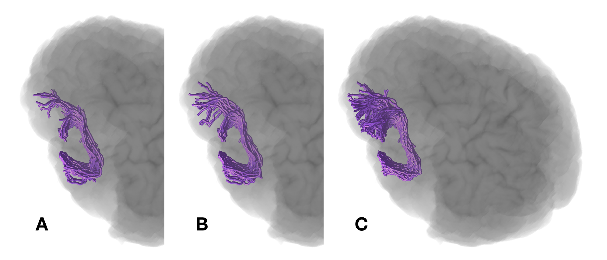
The information about the orientation of the fibers composing such anatomical structures can be estimated in-vivo by diffusion Magnetic Resonance Imaging (dMRI) techniques. By means of tractography, the paths of hundreds of thousands of fibers composing the white matter can be mathematically represented by 3D polylines called streamlines. White matter bundle segmentation aims to virtually group together streamlines that have an analogous shape and pass through the same anatomical brain regions into anatomically meaningful structures, known as bundles, e.g. the uncinate fasciculus (UF) (see Figure 2).

To overcome the limitations of manual segmentation [3, 4], which is very time consuming, in recent decades several automatic methods have been developed. They can be divided into two categories [5]: (i) connectivity-based, and (ii) streamline-based methods. Connectivity-based approaches aim to extract white matter bundles by means of predefined brain Region of Interest (ROIs) that the streamlines are supposed to pass (or not-pass) through [2, 6]. Streamline-based techniques are able to segment white matter bundles of interest by grouping together streamlines according to their geometrical similarity (clustering-based) [1, 7] or by exploiting the geometric information from previously segmented bundles, usually validated by experts, that are used as examples (example-based) [8, 5, 9]. Example-based methods have shown to outperform connectivity-based methods because these last ones strongly depend on the registration between subject and atlas and on the quality of the parcellation [5, 9]. Another disadvantage of connectivity-based techniques is that they do not take into account the shape of the streamlines, but only anatomical regions. On the other hand, clustering-based and example-based methods are based only on geometrical properties of the streamlines without considering any prior anatomical information about the bundle.

We aim to improve the results of bundle segmentation by considering information about both the shape of the streamlines and about the relative anatomical position of the bundle of interest. In order to achieve this goal, we propose to extend the example-based method proposed in [9], whose implementation is publicly available, by including additional anatomical information within the optimization process of the Linear Assignment Problem (LAP) [10]. Specifically, the extra information is given by taking into account the location of the endpoints of the streamlines and the proximity of the streamlines to specific anatomical ROIs predefined in the literature. We select [9] as a reference method since it is based on the LAP and has shown to provide better results than those based on the nearest-neighbor algorithm, such as [8] and [5].

Our contributions are the following: (i) to extend the work in [9] by including anatomical information in addition to the geometrical one, hence showing that it is possible to combine the best of streamline-based and connectivity-based methods; (ii) to show that small bundles are more difficult to be accurately segmented than large bundles and that anatomical information helps in reducing such difference.

We perform example-based bundle segmentation of 12 different bundles, each of them in 30 different subjects, for a total of 360 segmented bundles. We compare the proposed method with [9] by evaluating the results with the Dice Similarity Coefficient (DSC) to measure the overlap between the segmentation and the ground truth. We support scientific reproducibility and openness by publishing our methods as brainlife.io/apps.

In Section 2 we present the LAP method and the proposed extension, Section 3 contains the experiment design and the results, while Section 4 presents a short discussion.

2 Methods

2.1 Basic notation

We denote a streamline with a sequence of $n$ points as $s=(\mathbf{x}_{1},\ldots,\mathbf{x}_{n})$, where $\mathbf{x}_{i}\in\mathbb{R}^{3}$, $\forall i$. Usually, $n$ is in the order of $10^{1}-10^{2}$ and differs across streamlines. The entire set of streamlines of the white matter of a brain is known as the tractogram, $T=\{s_{1},\ldots,s_{M}\}$, where in general $M$ is in the order of $10^{5}-10^{6}$. A white matter bundle $b\subset T$, $b=\{s_{1},\ldots,s_{k}\}$, is a group of streamlines with a specific anatomical meaning, where $k\ll M$, and $k$ differs across bundles.

Several distance functions are available in the literature in order to quantify the geometrical distance between two streamlines. One of the most common is the Mean of Closest distances (MC) [7]: $d_{MC}(s_{a},s_{b})=\frac{d_{m}(s_{a},s_{b})+d_{m}(s_{b},s_{a})}{2}$ where $d_{m}(s_{a},s_{b})=\frac{1}{|s_{a}|}\sum_{\mathbf{x}_{i}\in s_{a}}\min_{\mathbf{x}_{j}\in s_{b}}\|\mathbf{x}_{i}-\mathbf{x}_{j}\|$ and $\|\cdot\|$ is the Euclidean distance.

2.2 The Linear Assignment Problem for Segmentation

Given two sets of objects, $A=\{a_{1},...a_{L}\}$ and $B=\{b_{1},...b_{L}\}$, and the cost matrix $C=\{c_{ij}\}_{ij}\in\mathbb{R}^{L\times L}$, where $c_{ij}$ is the cost of assigning $a^{A}_{i}$ to $b^{B}_{j}$, the Linear Assignment Problem (LAP) [10] aims to find the one-to-one correspondence between the objects in A and the objects in B by minimizing the total cost:

$$P^{*}=\operatorname*{argmin}_{P\in\mathcal{P}}\sum_{i,j=1}^{L}c_{ij}p_{ij}$$ (1)

where $P=\{p_{ij}\}_{ij}\in\mathcal{P}$ is a permutation matrix and $P^{*}$ is the optimal assignment. If multiple cost matrices need to be jointly optimized, they can be linearly combined. One of the most efficient algorithm to solve the LAP is the Jonker-Volgenant algorithm (LAPJV) [10].

In the case of example-based bundle segmentation, in [9] they consider the two sets of objects as being (i) the example bundle of $A$, $b^{A}=\{s_{1}^{A},\ldots,s_{k}^{A}\}$, and (ii) the tractogram of a subject $B$, $T^{B}=\{s_{1}^{B},\ldots,s_{M}^{B}\}$, from which we aim to segment the same anatomical bundle. The goal of bundle segmentation is to find the optimal correspondence of all the streamlines in $b^{A}$ with those in $T^{B}$. In [9], the cost matrix is equal to the distance matrix $D$ between the two sets of streamlines, in which each element is given by $c_{ij}=d_{MC}(s_{i}^{A},s_{j}^{B})$. Intuitively, the closer two streamlines are to each other, the more likely they belong to the same anatomical structure. The segmentation from multiple examples proposed in [9] is obtained by merging together the solution of multiple LAP solved individually. This is done through a refinement step that classifies the streamlines based on a majority rule.

2.3 Anatomically-Informed cost matrices

In order to include anatomical information into the LAP, we extend the cost matrix $D$ by adding two weighted anatomically-informed cost matrices: the endpoint-distance matrix $E$ and the ROI-based distance matrix $R$. Then, the new cost matrix becomes $C=\lambda_{D}D+\lambda_{E}E+\lambda_{R}R$.

2.3.1 Endpoint-based distance matrix

White matter fibers serve as connections between areas of the brain at their terminations. For this reason, from an anatomical and functional point of view, two streamlines with neighboring endpoints are assumed to play a similar role, regardless of their geometry. Based on this idea, we propose to build a new cost matrix $E$ by defining the endpoint-based distance, $d_{\text{END}}$, between two streamlines $s_{a}$ and $s_{b}$ as the mean Euclidean distance of their corresponding endpoints: $d_{\text{END}}(s_{a},s_{b})=\linebreak\frac{\min(\|\mathbf{x}_{1}^{a}-\mathbf{x}_{1}^{b}\|,\|\mathbf{x}_{1}^{a}-\mathbf{x}_{n_{b}}^{b}\|)+\min(\|\mathbf{x}_{n_{a}}^{a}-\mathbf{x}_{1}^{b}\|,\|\mathbf{x}_{n_{a}}^{a}-\mathbf{x}_{n_{b}}^{b}\|)}{2}$, where $\{\mathbf{x}_{1}^{a}$,$\mathbf{x}_{n_{a}}^{a}\}$ are the endpoints of $s_{a}$ and $\{\mathbf{x}_{1}^{b}$,$\mathbf{x}_{n_{b}}^{b}\}$ are those of $s_{b}$.

2.3.2 ROI-based distance matrix

Anatomically, bundles may be defined with respect to specific ROIs that they can cross or touch [3, 4, 2, 6]. Unfortunately, such regions cannot be easily and precisely defined in the subject space, but are often obtained by registration from an atlas, a step that is intrinsically limited by the inherent differences between the atlas and the specific subject. Nevertheless, such anatomical information is of primary importance. To create an additional cost matrix $R$ with such anatomical information, we first define the distance between a streamline and a single ROI, as the minimum Euclidean distance between them: $d_{min}(s,\text{ROI})=\min_{\mathbf{x}_{i}\in s,v_{j}\in\text{ROI}}\|\mathbf{x}_{i}-coord(v_{j})\|$, where $coord(v)$ are the 3D coordinates of the center of the voxel $v$ belonging to the ROI. Given a set of $N$ ROIs defining a bundle, the distance between a streamline and them can be defined as the average of the distances to each ROI. With such building block, we define the ROI-based distance between two streamlines $s_{a}$ and $s_{b}$, for a given set of ROIs as $d_{\text{ROIs}}=|\frac{1}{N}\sum_{i=1}^{N}d_{\text{min}}(s_{a},\text{ROI}_{i})-\frac{1}{N}\sum_{i=1}^{N}d_{\text{min}}(s_{b},\text{ROI}_{i})|$, meaning that two streamlines at similar distances from the ROIs are more likely to belong to the same anatomical structure.

3 Experiments

3.1 Materials

We randomly selected 130 healthy subjects from the publicly available Human Connectome Project (HCP) dMRI dataset [11] (90 gradients; b=2000; voxel size=1.25 mm isotropic). For each subject, tractograms of 750k streamlines were obtained using constrained spherical deconvolution (CSD) [12] and ensemble probabilistic tracking [13] (step size=0.625 mm, curvature parameters = 0.25, 0.5, 1, 2 and 4 mm).

Since example-based methods need accurate bundle segmentations to use both as example and to evaluate the results, we built a visually inspected ground truth dataset using a semi-automatic technique as follows. First, from each of the 130 tractograms, we segmented the 20 major associative bundles using the Automated Fiber Quantification (AFQ) algorithm [2]. Then, in order to have consistent bundles across subjects, given a bundle, we identified those that do not deviate more than the $20\%$ from the median number of streamlines, obtaining on average 50 segmentations per bundle. Finally, we visually inspected each segmentation and filtered out the outliers in order to have 30 segmentations per bundle. We then selected 12 bundles (6 left and 6 right) per subject, which we subdivided into two groups based on their number of streamlines: the small bundles are Cingulum Cingulate (CGCl and CGCr), Cingulum Hippocampus (CGHl and CGHr) and Uncinate Fasciculus (UFl and UFr), while the large bundles are Thalamic Radiation (TRl and TRr), Corticospinal tract (CSTl and CSTr) and Arcuate Fasciculus (AFl and AFr).

To evaluate the results of the proposed method, we measured the degree of overlap between the estimated bundle $\hat{b}^{B}$ and the true bundle $b^{B}$, using the Dice Similarity Coefficient (DSC) at the voxel-level: $DSC=2\frac{|v(\hat{b}^{B})\cap v(b^{B})|}{|v(\hat{b}^{B})|+|v(b^{B})|}$ where $v(b)$ is the set of voxels crossed by the streamlines of bundle $b$ and $|v(b)|$ is the number of voxels of $v(b)$.

3.2 Experimental design

We ran multiple experiments using the multiple LAP method of [9] (multi-LAP) and the proposed method (multi-LAP-anat) on a total of 360 segmented bundles. In both cases, each pair of tractograms were aligned with an initial affine registration. We used an example set composed of 5 bundles, since it was proved that considering a larger example set has no substantial impact on the final result of the segmentation [9]. In the multi-LAP-anat method, we added the two anatomically-informed distance matrices to the original cost matrix as explained in section 2.3. The parameters of $\lambda_{D}$, $\lambda_{E}$ and $\lambda_{R}$ were set in order to let all the values of the matrices span in the same range (which would approximately correspond to $\lambda_{D}=1$, $\lambda_{E}=0.4$ and $\lambda_{R}=1.6$). To build the ROI-based distance matrix, for each bundle, we considered the two waypoint ROIs that delineate the trajectory of the bundle before it diverges towards the cortex that are defined in [4], and we transferred them in the individual subject space through a non-linear registration. We then compared the performances of the two methods through the DSC score.

All the experiments were developed in Python code and ran using cloud computing resources provided by brainlife.io. Code and dataset are freely available for reproducibility at https://doi.org/10.25663/brainlife.app.122 and https://doi.org/10.25663/brainlife.pub.3 respectively.

3.3 Results

In Table 1 we separately report the mean DSC results for the two methods that we compared across all 30 subjects, for both small and large bundles. For the small bundles, with the multi-LAP method we observed a standard deviation of the mean between $0.009$ and $0.015$, and with the proposed multi-LAP-anat method between $0.007$ and $0.011$. For the large bundles, both methods registered a standard deviation of the mean $\leq 0.005$.

	CGCl	CGCr	CGHl	CGHr	UFl	UFr
multi-LAP	0.81	0.82	0.77	0.76	0.74	0.76
multi-LAP-anat	0.83	0.86	0.83	0.80	0.80	0.81

	TRl	TRr	CSTl	CSTr	AFl	AFr
multi-LAP	0.85	0.85	0.84	0.85	0.83	0.80
multi-LAP-anat	0.87	0.87	0.86	0.87	0.86	0.84

Table 1: Mean DSC across 30 subjects for both the 6 small bundles and the 6 large bundles for the two methods compared.

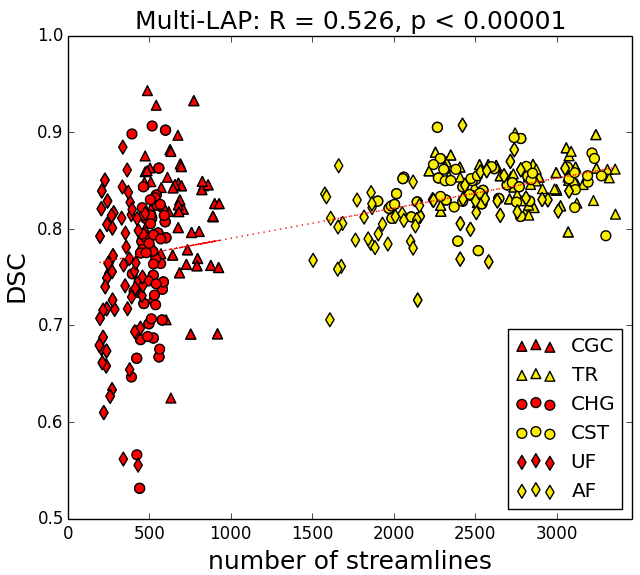
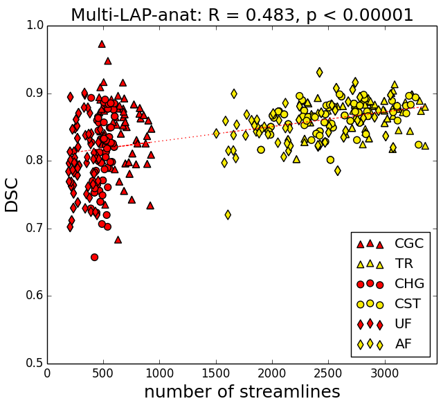
Figure 2 illustrates the individual DSC scores as a function of bundle size in terms of number of streamlines, for the small and large bundles and for the two methods compared.

Fig. 1: DSC as a function of bundle size using the multi-LAP method [9] (left panel) and using the proposed multi-LAP-anat method (right panel). In red the small bundles and in yellow the large bundles, 30 examples for each bundle.

Fig. 2: Comparative paradigmatic example of a segmented uncinate fasciculus (UF) obtained with A) the multi-LAP method [9], B) the proposed multi-LAP-anat method and C) the ground truth.

4 Discussion

Table 1 illustrates that, on average, the proposed multi-LAP-anat method outperforms the multi-LAP method of [9], for all the bundles considered. In all the cases we obtained a mean DSC between 0.80 and 0.87, which means that the overlap with the ground truth is at least 80%. Streamlines composing the same anatomical bundle not only have a similar shape, but are also characterized by their propensity to interconnect or pass through predefined ROIs of the brain. Including such information into the optimization process is useful in particular in identifying those streamlines that may have a less similar shape from the example, but that are close to ROIs that are known from the literature pertaining to the bundle of interest. Moreover, also taking into account the endpoint-based distance helps to select all the streamlines that end in the same terminal region. Figure 2 shows a paradigmatic example in which the multi-LAP-anat method correctly identifies most of the streamlines terminating in the cortical areas, which instead are partially missing in the bundle segmented by the multi-LAP method.

Table 1 (first row) and Figure 2 (left panel) provide evidence that small bundles, which are usually more sensitive to registration errors, are generally harder to segment than large bundles. Using the proposed multi-LAP-anat method, we obtain a mean improvement in the DSC score of $+4.5\%$ for the small bundles, see Table 1. In these cases, we also notice a decreased variance when using the proposed method, which can be seen from the comparison in Figure 2, where the vertical dispersion of the red points is narrower in the right panel.

The proposed method also improves the results for large bundles, for which we observe a mean improvement in the DSC score of $+2.5\%$, see Table 1. These results confirm the assumption that, for all the bundles considered, including additional information about the relative anatomical position of bundles helps to improve the example-based bundle segmentation.

References

- [1] Lauren J. O’Donnell and Carl-Fredrik F. Westin, “Automatic tractography segmentation using a highdimensional white matter atlas,” in IEEE Trans. Med. Imag, 2007, pp. 1562–1575.
- [2] Jason D. Yeatman, Robert F. Dougherty, Nathaniel J. Myall, Brian A. Wandell, and Heidi M. Feldman, “Tract Profiles of White Matter Properties: Automating Fiber-Tract Quantification,” PLoS ONE, vol. 7, no. 11, pp. e49790+, Nov. 2012.
- [3] Marco Catani, Robert J. Howard, Sinisa Pajevic, and Derek K. Jones, “Virtual in vivo interactive dissection of white matter fasciculi in the human brain.,” NeuroImage, vol. 17, no. 1, pp. 77–94, Sept. 2002.
- [4] Setsu Wakana, Arvind Caprihan, Martina M. Panzenboeck, James H. Fallon, Michele Perry, Randy L. Gollub, Kegang Hua, Jiangyang Zhang, Hangyi Jiang, Prachi Dubey, Ari Blitz, Peter van Zijl, and Susumu Mori, “Reproducibility of quantitative tractography methods applied to cerebral white matter.,” NeuroImage, vol. 36, no. 3, pp. 630–644, July 2007.
- [5] Eleftherios Garyfallidis, Marc-Alexandre A. Côté, Francois Rheault, Jasmeen Sidhu, Janice Hau, Laurent Petit, David Fortin, Stephen Cunanne, and Maxime Descoteaux, “Recognition of white matter bundles using local and global streamline-based registration and clustering.,” NeuroImage, vol. 170, pp. 283–295, Apr. 2018.
- [6] Demian Wassermann, Nikos Makris, Yogesh Rathi, Martha Shenton, Ron Kikinis, Marek Kubicki, and Carl-Fredrik F. Westin, “The white matter query language: a novel approach for describing human white matter anatomy.,” Brain structure & function, vol. 221, pp. 4705–4721, Jan. 2016.
- [7] Song Zhang, S. Correia, and D. H. Laidlaw, “Identifying White-Matter Fiber Bundles in DTI Data Using an Automated Proximity-Based Fiber-Clustering Method,” IEEE Transactions on Visualization and Computer Graphics, vol. 14, no. 5, pp. 1044–1053, Sept. 2008.
- [8] Sang W. Yoo, Pamela Guevara, Yong Jeong, Kwangsun Yoo, Joseph S. Shin, Jean-Francois Mangin, and Joon-Kyung Seong, “An Example-Based Multi-Atlas Approach to Automatic Labeling of White Matter Tracts,” PloS one, vol. 10, no. 7, 2015.
- [9] Nusrat Sharmin, Emanuele Olivetti, and Paolo Avesani, “White Matter Tract Segmentation as Multiple Linear Assignment Problems,” Frontiers in Neuroscience, vol. 11, Feb. 2018.
- [10] J. Bijsterbosch and A. Volgenant, “Solving the Rectangular assignment problem and applications,” Annals of Operations Research, vol. 181, pp. 443–462, June 2010.
- [11] Stamatios N. Sotiropoulos, Saad Jbabdi, Junqian Xu, Jesper L. Andersson, Steen Moeller, Edward J. Auerbach, Matthew F. Glasser, Moises Hernandez, Guillermo Sapiro, Mark Jenkinson, David A. Feinberg, Essa Yacoub, Christophe Lenglet, David C. Van Essen, Kamil Ugurbil, Timothy E. Behrens, and WU-Minn HCP Consortium, “Advances in diffusion MRI acquisition and processing in the Human Connectome Project.,” NeuroImage, vol. 80, pp. 125–143, Oct. 2013.
- [12] J-Donald Tournier, Fernando Calamante, and Alan Connelly, “Robust determination of the fibre orientation distribution in diffusion MRI: Non-negativity constrained super-resolved spherical deconvolution,” NeuroImage, vol. 35, no. 4, pp. 1459–1472, May 2007.
- [13] Hiromasa Takemura, Cesar F. Caiafa, Brian A. Wandell, and Franco Pestilli, “Ensemble Tractography.,” PLoS computational biology, vol. 12, no. 2, Feb. 2016.