Spectral analysis of the hybrid PG 1159-type central stars
of the planetary nebulae Abell 43 and NGC 7094

Abstract

Stellar post asymptotic giant branch (post-AGB) evolution can be completely altered by a final thermal pulse (FTP) which may occur when the star is still leaving the AGB (AFTP), at the departure from the AGB at still constant luminosity (late TP, LTP) or after the entry to the white-dwarf cooling sequence (very late TP, VLTP). Then convection mixes the He-rich material with the H-rich envelope. According to stellar evolution models the result is a star with a surface composition of $\mathrm{H}\approx\,20$ % by mass (AFTP), $\approx 1$ % (LTP), or (almost) no H (VLTP). Since FTP stars exhibit intershell material at their surface, spectral analyses establish constraints for AGB nucleosynthesis and stellar evolution. We performed a spectral analysis of the so-called hybrid PG 1159-type central stars (CS) of the planetary nebulae Abell 43 and NGC 7094 by means of non-local thermodynamical equilibrium models. We confirm the previously determined effective temperatures of $\mbox{$T_{\mathrm{eff}}$}=115\,000\pm 5\,000\,\mathrm{K}$ and determine surface gravities of $\log(g\,/\,\mathrm{cm/s^{2}})=5.6\pm 0.1$ for both. From a comparison with AFTP evolutionary tracks, we derive stellar masses of $0.57^{+0.07}_{-0.04}$ $M_{\odot}$ and determine the abundances of H, He, and metals up to Xe. Both CS are likely AFTP stars with a surface H mass fraction of $0.25\pm 0.03$ and $0.15\pm 0.03$, respectively, and a Fe deficiency indicating subsolar initial metallicities. The light metals show typical PG 1159-type abundances and the elemental composition is in good agreement with predictions from AFTP evolutionary models. However, the expansion ages do not agree with evolution timescales expected from the AFTP scenario and alternatives should be explored.

1 Introduction

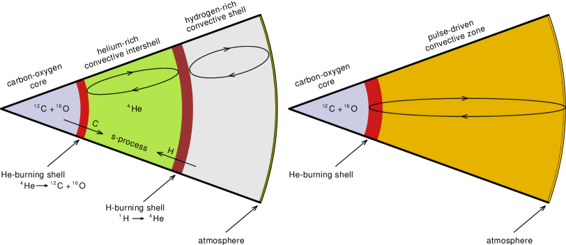
Figure 1: Left: Internal structure (not to scale) of an AGB star during a thermal pulse. Right: Internal structure of a post-AGB star after having experienced a final thermal pulse that caused flash induced mixing of the envelope and the intershell region.

Asymptotic giant branch (AGB) stars are important contributors to the formation of elements heavier than iron (trans-iron elements, TIEs). Schematically, the internal structure of an AGB star is illustrated in Fig. 1. It is composed of an inner C/O core, the two burning shells with a He, C, and O rich intershell region in between and an H-rich convective envelope on top. These stars experience several thermal pulses (TPs) during which the intershell region becomes convectively unstable and C-rich both due to He burning and to dredge up from the core. Additionally, small amounts of H can be partially mixed into the intershell region during the expansion and cooling of the envelope that follows a TP. The presence of large amounts of ¹²C mixed with traces of H at high temperatures leads to the formation of ¹³C that acts as a neutron source for the slow neutron capture process (s-process). The intershell region of AGB stars is the main astrophysical site for the s-process. The stellar post-AGB evolution divides into two major channels of H-rich and H-deficient stars. The latter comprise about a quarter of all post-AGB stars and include He- and C-dominated stars. While the He-dominated, H-deficient stars may be the result of stellar mergers (Reindl et al. 2014b), it is commonly accepted that the C-rich are the outcome of a (very) late He-shell flash (late thermal pulse, LTP, cf. Werner & Herwig 2006). The occurrence of a thermal pulse in a post-AGB star or white dwarf was predicted by, e.g., Paczyński (1970), Schönberner (1979), and Iben et al. (1983). The particular timing of the final thermal pulse (FTP), determines the amount of remaining photospheric H (cf., Herwig 2001). Still on the AGB (AGB final thermal pulse, AFTP), flash-induced mixing of the H-rich envelope ($\approx 10^{-2}\,M_{\odot}$) with the He-rich intershell layer ($\approx 10^{-2}\,M_{\odot}$) reduces the H abundance to about $10-20$ % but H i lines remain detectable. After the departure from the AGB, the H-rich envelope is less massive ($10^{-4}\,M_{\odot}$). If the nuclear burning is still “on”, i.e., the star evolves at constant luminosity, the mixing due to a late thermal pulse (LTP) reduces H below the detection limit (about 10 % by mass at the relatively high surface gravity). After the star has entered the white-dwarf cooling sequence and the nuclear burning is “off”, a very late thermal pulse (VLTP) will produce convective mixing of the entire H-rich envelope (no entropy barrier due to the H-burning shell) down to the bottom of the He-burning shell where H is burned. In that case, the star will become H free at that time. The internal structure of such a post-AGB star that underwent a FTP scenario is illustrated in Fig. 1.
The spectroscopic class of PG 1159 stars (effective temperatures of $75\,000\,\mathrm{K}\la\mbox{$T_{\mathrm{eff}}$}\la 250\,000\,\mathrm{K}$ and surface gravities of $5.5\la\log(g\,/\,\mathrm{cm/s^{2}})\la 8.0$) belongs to the H-deficient, C-rich evolutionary channel (e.g., Werner & Herwig 2006), with the sequence AGB $\rightarrow$ [WC]-type Wolf-Rayet stars $\rightarrow$ PG 1159 stars $\rightarrow$ DO-type white dwarfs (WDs). In the AFTP and LTP scenarios with any remaining H, the stars will turn into DA-type WDs. In PG 1159 star photospheres, He, C, and O are dominant with mass fractions of He = [0.30,0.92], C = [0.08,0.60], and O = [0.02,0.20] (Werner et al. 2016).
Napiwotzki & Schönberner (1991) discovered the spectroscopic sub-class of so-called hybrid PG 1159 stars. They found that WD 1822+008 (McCook & Sion 1999a, b), the central star (CS) of the planetary nebula (PN) Sh 2-68 exhibits strong Balmer lines in its spectrum. The hybrid PG 1159 stars are thought to be AFTP stars. Presently, only five of them are known, namely the CSPNe of Abell 43, NGC 7094, Sh 2$-$68, HS 2324+3944, and SDSS 152116.00+251437.46 (Werner & Herwig 2006; Werner et al. 2014).
Abell 43 (PN G036.0+17.6) was discovered by Abell (1955, object No. 31) and classified as PN (Abell 1966, No. 43). NGC 7094 (PN G066.7$-$28.2) was discovered in 1885 by Swift (1885). Kohoutek (1963) identified it as a PN (K 1$-$19). Narrow-band imaging of Abell 43 and NGC 7094 (Rauch 1999) revealed apparent sizes (in West-East and North-South direction) of 1′28″ $\times$ 1′20″and 1′45″ $\times$ 1′46″, respectively.
Abell 43 and NGC 7094 belong to the group of so-called “Galactic Soccerballs” (Rauch 1999) because they exhibit filamentary structures that remind of the seams of a traditional leather soccer ball. These structures may be explained by instabilities in the dense, moving nebular shell (Vishniac 1983). While Abell 43 is almost perfectly round and most likely expanded into a void in the ISM, NGC 7094 shows some deformation that may be a hint for ISM interaction. Another recently discovered member of this group is the PN Kn 61 (SDSS J192138.93+381857.2, Kronberger et al. 2012; De Marco et al. 2015). García-Díaz et al. (2014) compared medium-resolution optical spectra of the CSPN Kn 61 with spectra published by Werner et al. (2014) and found a particularly close resemblance of the CSPN Kn 61 to SDSS 075415.12+085232.18, an H-deficient PG 1159-type star with $\mbox{$T_{\mathrm{eff}}$}=120\,000\pm 10\,000\,\mathrm{K}$, $\log g=7.0\pm 0.3$, and a mass ratio C/He = 1. Other members and candidates to become a Galactic Soccerball nebula are known, e.g., the PN NGC 1501 (PN G144.5+06.5). An investigation on the 3-dimensional ionization structure by Ragazzoni et al. (2001) had shown that it might resemble a Soccerball nebula in a couple of thousands of years. The CSPN, however, is of spectral type [WC4] (Koesterke & Hamann 1997) and cannot resemble a progenitor star of the CSs of Abell 43 and NGC 7094. In this paper, we analyze the hybrid PG 1159-type CSs of Abell 43 and NGC 7094, that we introduce briefly in the following paragraphs.
A first spectral analysis of the CSs of Abell 43 and NGC 7094, namely WD 1751+106 and WD 2134+125 (McCook & Sion 1999a, b), respectively, with non-local thermodynamical equilibrium (NLTE) model atmospheres that considered opacities of H, He, and C was presented by Dreizler et al. (1995). They analyzed medium-resolution optical spectra and found that their synthetic spectra, calculated with $\mbox{$T_{\mathrm{eff}}$}=110\,000\,\mathrm{K}$, $\log g=5.7$, and a surface-abundance pattern of H/He/C = 42/51/5 (by mass, H is uncertain), reproduced equally good the observations of both stars making them a pair of spectroscopic twins.
Napiwotzki (1999) used medium-resolution optical spectra and an extended H+He-composed NLTE model-atmosphere grid. With a statistical ($\chi^{2}$) approach, he found $\mbox{$T_{\mathrm{eff}}$}=116\,900\pm 5500\,\mathrm{K}$ and $\log g=5.51\pm 0.22$ for WD 1751+106 and $\mbox{$T_{\mathrm{eff}}$}=125\,900\pm 7700\,\mathrm{K}$ and $\log g=5.45\pm 0.23$ for WD 2134+125. An attempt to measure the Fe abundance of WD 2134+125 from far ultraviolet (FUV) observations performed with Far Ultraviolet Spectroscopic Explorer (FUSE) revealed a strong Fe underabundance of 1-2 dex (Miksa et al. 2002). This was not in line with expectations from stellar evolution theory (e.g., Busso et al. 1999). Ziegler et al. (2009) found also an underabundance of Ni of about 1 dex for both stars. The transformation of Fe to Ni seems therefore unlikely to be the reason for the Fe deficiency. They reanalyzed $T_{\mathrm{eff}}$ and $\log g$ of WD 2134+125 and found $\mbox{$T_{\mathrm{eff}}$}=100\,000\pm 15\,000\,\mathrm{K}$ and $\log g=5.5\pm 0.2$ with an improved abundance ratio of H/He = 17/69 (by mass). Furthermore, the element abundances of the C – Ne, Si, P, and S were determined. Ringat et al. (2011) reanalyzed WD 1751+106 and found $\mbox{$T_{\mathrm{eff}}$}=105\,000\pm 10\,000\,\mathrm{K}$ and $\log g=5.6\pm 0.3$. Also the element abundances of C – Ne, Si, P, and S were determined and agree with the values of Friederich (2010). Löbling (2018) found $\mbox{$T_{\mathrm{eff}}$}=115\,000\pm 5000\,\mathrm{K}$ for both stars and $\log g=5.4\pm 0.1$ and $\log g=5.5\pm 0.1$ for WD 2134+125 and WD 1751+106, respectively. She considered 31 elements in her analysis and determined abundances in individual line-formation calculations. The present work is a continuative analysis giving a more extensive description.
For NLTE model-atmosphere calculations, reliable atomic data is mandatory to construct detailed model atoms to represent individual elements. In the last decade, the availability of such atomic data improved, e.g., Kurucz’s line lists for iron-group elements (IGEs), namely Ca - Ni, were strongly extended in 2009 (Kurucz 2009, 2011) by about a factor of ten. In addition, transition probabilities and oscillator strengths for many TIEs were calculated recently (Table 6). Therefore, we decided to perform a detailed spectral analysis of the hybrid PG 1159-type CSPNe Abell 43 and NGC 7094, by means of state-of-the-art NLTE model-atmosphere techniques. We describe the available observations and our model atmospheres in Sects. 2 and 3, respectively. The spectral analyses follow in Sects. 4 and 5. We investigate on the stellar wind of both stars in Sect. 6 and determine stellar masses, distances, and luminosities in Sect. 7. We summarize the results and conclude in Sect. 8.

2 Observations

Our spectral analysis is based on high signal-to-noise ratio ($S/N$) and high-resolution observations from the far ultraviolet (FUV) to the optical wavelength range. UV spectra were retrieved from the Barbara A. Mikulski Archive for Space Telescopes (MAST). To improve the $S/N$, multiple observations in the same setup were co-added. The spectra were partly processed with a low-pass filter (Savitzky & Golay 1964). To simulate the instruments’ resolutions, all synthetic spectra shown in this paper are convolved with respective Gaussians. The observation log for all space and ground based observations of WD 1751+106 and WD 2134+125 used for this work is given in Table 5.

Radial and rotational velocity.

We measured radial velocity shifts for all observations using prominent lines of He II, C IV, O V and vi, Si V, and Fe VII and shifted the spectra to rest wavelength.
The observed line profiles are broadened but the quality of the spectra does not unambiguously allow to decide whether it is due to stellar rotation or caused by some wind related macro turbulence. For WD 1751+106, we selected O VI $\lambda\lambda\,1124.7,1124.9$ Å and S VI $\lambda\,1117.8$ Å (Fig. 2) to determine a rotational velocity of $v_{\mathrm{rot}}\sin i=18\pm 5\,\mathrm{km}/\mathrm{s}$. This new determination revises the previous higher value of $v_{\mathrm{rot}}\sin i=42\pm 13\,\mathrm{km}/\mathrm{s}$ (Rauch et al. 2004). The profiles of these lines also agree with broadening with radial-tangential macro turbulence profiles (Gray 1975) with the same velocity (Fig. 2). For WD 2134+125, we used O VI $\lambda\lambda\,1122.4,1122.6,1124.7,1124.9$ and N V $\lambda\,1242.6$ Å (Fig. 2) to determine $v_{\mathrm{rot}}\sin i=28\pm 5\,\mathrm{km}/\mathrm{s}$. This value agrees within the error limits with the value of $46\pm 16\,\mathrm{km}/\mathrm{s}$ from Rauch et al. (2004). Again, we cannot claim this broadening to be rotation alone because the profiles can also be reporduced with radial-tangential macro turbulence profiles with $v_{\mathrm{macro}}=35\pm 5\,\mathrm{km}/\mathrm{s}$.

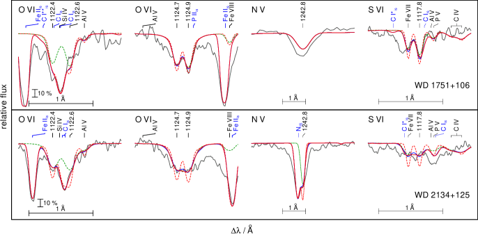
Figure 2: Synthetic spectra (red) convolved with rotational profiles ($v_{\mathrm{rot}}=18\,\mathrm{km}/\mathrm{s}$ for WD 1751+106, upper panels and $v_{\mathrm{rot}}=28\,\mathrm{km}/\mathrm{s}$ for WD 2134+125, lower panels) and convolved with radial-tangential macro turbulence profiles (blue, $v_{\mathrm{macro}}=18\,\mathrm{km}/\mathrm{s}$ for WD 1751+106, upper panels and $v_{\mathrm{macro}}=35\,\mathrm{km}/\mathrm{s}$ for WD 2134+125, lower panels) around O vi, N v, and S vi lines (marked with their wavelengths at the top of the panels) calculated from our final models compared with observations (gray). A model without extra broadening (red, dashed) and one without interstellar absorption (green, dashed) are shown. Interstellar absorption lines are indicated by blue marks.

Interstellar reddening

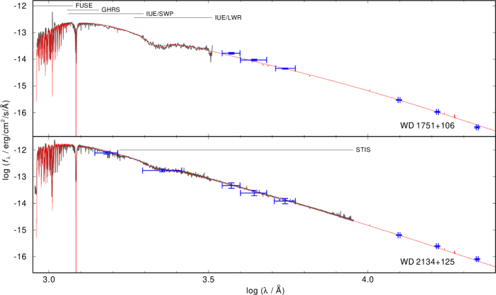
Figure 13: Determination of $E_{\mathrm{B-V}}$. Synthetic spectra of our best models (thick, red lines) of WD 1751+106 (top panel, interstellar reddening with $\mbox{$E_{\mathrm{B-V}}$}=0.265$ was applied) and WD 2134+125 (bottom, $\mbox{$E_{\mathrm{B-V}}$}=0.135$) compared with the observations (black). The model fluxes are normalized to the 2MASS J magnitude (Cutri et al. 2003). U, B, and V magnitudes from Acker et al. (1992) and GALEX FUV and NUV magnitudes (blue crosses) from Bianchi et al. (2011) were added for WD 2134+125 (flux conversion: https://asd.gsfc.nasa.gov/archive/galex/FAQ/counts_background.html). Interstellar line absorption is included in the FUSE spectral range of the models.

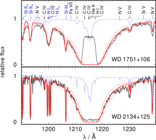
Figure 21: Synthetic spectra of our best models (red lines) for WD 1751+106 (top panel) and WD 2134+125 (bottom) around H I Ly $\alpha$ calculated with $n_{\mathrm{H\,I}}=1.0\times 10^{21}\,\mathrm{cm^{-2}}$ and $6.5\times 10^{20}\,\mathrm{cm^{-2}}$, respectively, compared with the observations (gray). Models with $\Delta n_{\mathrm{H\,I}}=2.0\times 10^{20}\,\mathrm{cm^{-2}}$ are shown (red, dashed). Spectra without interstellar absorption are shown for comparison (blue, dashed).

was measured by a comparison of observed UV fluxes and optical and infrared brightnesses with our synthetic spectra. The latter were normalized to the Two Micron All Sky Survey (2MASS, Skrutskie et al. 2006; Cutri et al. 2003) brightnesses and then, Fitzpatrick’s law (Fitzpatrick 1999) was applied to match the observed UV continuum flux level (Fig. 13). We determined $\mbox{$E_{\mathrm{B-V}}$}=0.265\pm 0.01$ and $\mbox{$E_{\mathrm{B-V}}$}=0.135\pm 0.01$ for WD 1751+106 and WD 2134+125, respectively.
We determined the interstellar neutral H column density from the comparison of theoretical line profiles of Ly $\alpha$ with the observations (Fig. 21). These are best reproduced at $n_{\text{H\,{i}}}=1.0\pm 0.1\times 10^{21}\,\mathrm{cm^{-2}}$ and $n_{\text{H\,{i}}}=6.5\pm 0.1\times 10^{20}\,\mathrm{cm^{-2}}$ for WD 1751+106 and WD 2134+125, respectively. Our values of $\log(n_{\mathrm{\text{H\,{i}}}}/\mbox{$E_{\mathrm{B-V}}$})=21.58\pm 0.02$ and $\log(n_{\mathrm{\text{H\,{i}}}}/\mbox{$E_{\mathrm{B-V}}$})=21.68\pm 0.03$, respectively, agree well with the prediction from the Galactic reddening law of Groenewegen & Lamers (1989, $\log(n_{\mathrm{\text{H\,{i}}}}/\mbox{$E_{\mathrm{B-V}}$})=21.58\pm 0.1$).

Interstellar line absorption

in the FUSE observations was modeled with the line-profile fitting procedure OWENS (Lemoine et al. 2002; Hébrard et al. 2002; Hébrard & Moos 2003). It allows to consider several individual clouds in the interstellar medium (ISM) with individual chemical compositions, column densities for each of the included molecules and ions, radial and turbulent velocities, and temperatures. The FUV observations are strongly contaminated by ISM line absorption and, thus, it is necessary to reproduce these lines well to unambiguously identify photospheric lines (cf., Ziegler et al. 2007, 2012). In the FUSE spectra of WD 1751+106 and WD 2134+125, ISM absorption lines from $\mathrm{H}_{2}$ ($\mathrm{J}=0-5$), HD, C i-iii, N i-ii, O i, Si ii, P ii, S iii, Ar i, and Fe ii were identified and simulated.

3 Model atmospheres and atomic data

To calculate synthetic spectra, we used the Tübingen NLTE Model Atmosphere Package (TMAP, Werner et al. 2003, 2012). The models assume plane-parallel geometry, are chemically homogeneous, and in hydrostatic and radiative equilibrium. TMAP considers level dissolution (pressure ionization) following Hummer & Mihalas (1988) and Hubeny et al. (1994). Stark-broadening tables of Tremblay & Bergeron (2009, extended tables of 2015, priv. comm.) and Schöning & Butler (1989) are used to calculate the theoretical profiles of H i and He ii lines, respectively. To represent the elements considered by TMAP, model atoms were retrieved from the Tübingen Model Atom Database (TMAD, Rauch & Deetjen 2003) that has been constructed as part of the Tübingen contribution to the German Astrophysical Virtual Observatory (GAVO). For IGEs and TIEs (atomic weight $Z\geq 29$), we used Kurucz’s line lists (Kurucz 2009, 2011) and recently calculated data for Zn, Ga, Ge, Se, Kr, Sr, Zr, Mo, Te, I, Xe, and Ba (Table 6) that is available via the Tübingen Oscillator Strengths Service (TOSS). For the elements with $Z\geq 20$, we created model atoms using a statistical approach that calculates super levels and super lines (Rauch & Deetjen 2003). The statistics of all elements considered in our model-atmosphere calculations are summarized in Table 4.
To simulate prominent P Cygni profiles in the observations, we used the Potsdam Wolf-Rayet (PoWR) code that has been developed for expanding atmospheres and considers mass loss due to a stellar wind (Sect.6). These models are used to determine mass loss rates and terminal wind velocities.

4 Effective temperature and surface gravity

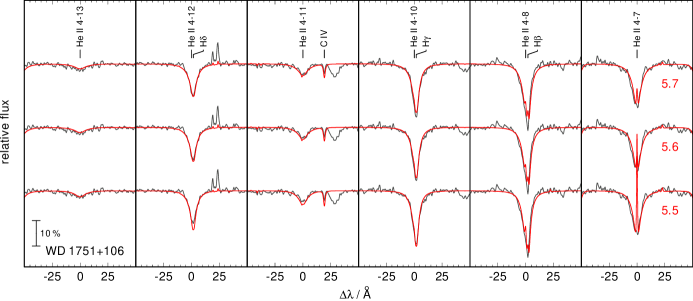
Figure 14: Synthetic spectra calculated with $\mbox{$T_{\mathrm{eff}}$}=115\,000\,\mathrm{K}$ and different $\log g$, compared with the UVES SPY observations of He ii and H i lines for WD 1751+106 (gray). ($\log g$ is indicated in panel 6)

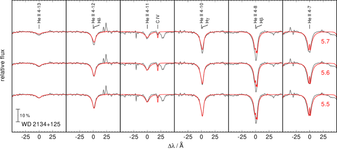
Figure 15: Synthetic spectra calculated with $\mbox{$T_{\mathrm{eff}}$}=115\,000\,\mathrm{K}$ and different $\log g$, compared with the UVES SPY observations of He ii and H i lines for WD 2134+125 (gray). ($\log g$ is indicated in panel 6)

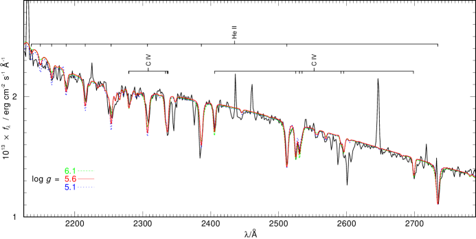
Figure 16: Section of the HST/STIS spectrum of WD 2134+125 (black) compared with synthetic spectra calculated with $\mbox{$T_{\mathrm{eff}}$}=115\,000\,\mathrm{K}$ and different $\log g$ of 6.1 (green dashed), 5.6 (red solid), and 5.1 (blue dotted).

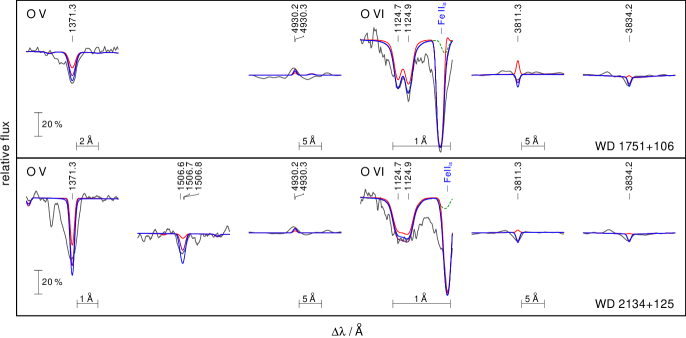
Figure 17: Synthetic spectra calculated with $\log g=5.6$ for WD 1751+106 (top panel) and WD 2134+125 (bottom) and different $T_{\mathrm{eff}}$ (red: $\mbox{$T_{\mathrm{eff}}$}=125\,000\,\mathrm{K}$, purple: $\mbox{$T_{\mathrm{eff}}$}=115\,000\,\mathrm{K}$, blue: $\mbox{$T_{\mathrm{eff}}$}=105\,000\,\mathrm{K}$), compared with the STIS observation of O v $\lambda\,1371.3$ Å and the FUSE observation of O vi $\lambda\lambda\,1124.7,1124.9$ Å (gray). A model without interstellar absorption (green, dashed) is shown in addition.

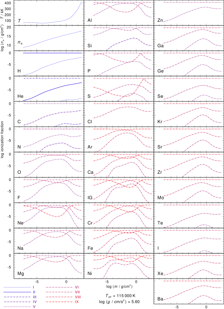
Figure 20: Temperature and density structures and ionization fractions of all ions which are considered in our final model for WD 2134+125.

Model atmospheres grids ($\Delta\mbox{$\mbox{$T_{\mathrm{eff}}$}=5000\,\mathrm{K}$}$ and $\Delta\mbox{$\log g=0.1$}$) were calculated around the literature values of Löbling (2018). These models consider opacities of 31 elements from H to Ba for which the ionization fractions of the considered ions are shown in Fig. 20. The abundances used for the calculation of the atmospheric structure are given in Table 7. The best agreement for the line width and depth increment for the observed He ii $\lambda\lambda\,4025.6,4100.1,4199.8,4338.7,4859.3,5411.5$ Å, and H i $\lambda\lambda\,4101.7,4340.5,4861.3$ Å was obtained for surface gravity values of $\log g=5.6\pm 0.1$ for WD 1751+106 (Fig. 14) and WD 2134+125 (Fig. 15). The value for WD 2134+125 is also verified by the depth increment of the He II Fowler series (Fig. 16). The lower surface gravity values of Löbling (2018) were based on model atmospheres assuming the abundances found by Friederich (2010). Using new models with a revised He/H ratio and including opacities of more elements, these previous values appear too low. Higher values for $\log g$ have an impact on the final masses which are lower compared to previous values (Sect. 7). We confirm the temperature determination of $\mbox{$T_{\mathrm{eff}}$}=115\,000\pm 5\,000\,\mathrm{K}$ for both stars by Löbling (2018) by the evaluation of the O V/O VI ionization equilibrium using O v $\lambda\,1371.3,1506.6,1506.7,1506.8,4930.2,4930.3$ Å and O vi $\lambda\lambda\,1124.7,1124.9,3811.3,3834.2$ Å (Fig. 17). We adopt $\mbox{$T_{\mathrm{eff}}$}=115\,000\,\mathrm{K}$ and $\log g=5.6$ for WD 1751+106 and WD 2134+125 for our further analysis.

5 Metal abundances

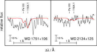
Figure 6: Synthetic spectra around Ar viii $\lambda\,1164.1$ Å calculated from our final models compared with the FUSE observations.

In the following paragraphs, we discuss all elements, that were considered in this analysis. To determine the abundances, we varied them in subsequent line formation calculations in steps of 0.2 dex or smaller. The abundances were derived by line-profile fits and evaluation by eye. For illustration, some representative spectral lines are shown in Figs. 3-7. These values are affected by typical errors estimated to 0.3 dex by redoing the abundance determination for models at the edges of the error range for $T_{\mathrm{eff}}$ and $\log g$ (we used a model with $\mbox{$T_{\mathrm{eff}}$}=120\,000\,\mathrm{K}$, $\log g=5.5$ and one with $\mbox{$T_{\mathrm{eff}}$}=110\,000\,\mathrm{K}$ and $\log g=5.7$). If no line identification was possible, we determined upper limits by reducing the abundance until the strongest computed lines become undetectable within the noise of the spectrum. The results are summarized in Table 3. The whole FUSE spectra compared with our final models are shown in Fig. 18 and the GHRS spectrum of WD 1751+106 as well as the STIS spectrum of WD 2134+125 in Fig. 19. The solar abundances are taken from Asplund et al. (2009); Scott et al. (2015b, a); Grevesse et al. (2015).

Carbon.

Detailed line-profile fits were performed for C IV $\lambda\lambda\,1168.9,1169.0,1184.6$ Å in the FUSE observations, C IV $\lambda\lambda\,1351.2,1351.3,1353.0$ Å in the GHRS or STIS observations, and the C iv lines at $3685-3691$ Å, $4440-4442$ Å, $4785-4790$ Å, $5016-5019$ Å, and $6591-6593$ Å in the UVES SPY observations (Fig. 3). We achieve $[\mathrm{C}]=\log\,\mathrm{(abundance/solar\ abundance)}={\color[rgb]{0,0,0}2.0}$ for WD 1751+106 and $[\mathrm{C}]={\color[rgb]{0,0,0}2.1}$ for WD 2134+125.

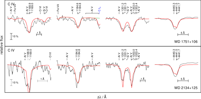
Figure 3: Synthetic spectra (red) around C iv lines calculated from our final model compared with observations (gray).

Nitrogen.

The photospheric N V $\lambda\lambda\,1238.8,1242.8$ Å resonance doublet in the STIS spectrum of WD 2134+125 is blended by strong interstellar absorption. Therefore, we used N V $\lambda\lambda\,4943.2,4944.0,4945.34945.6,4945.7$ Å in addition (Fig. 4) and determined $[\mathrm{N}]={\color[rgb]{0,0,0}0.6}$ for WD 1751+106 and $[\mathrm{N}]={\color[rgb]{0,0,0}-0.3}$ for WD 2134+125.

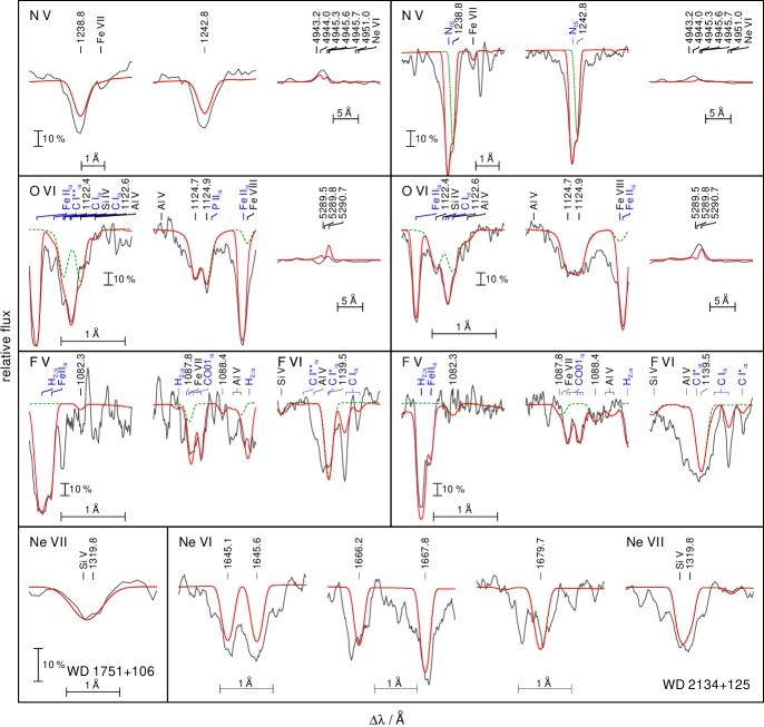
Figure 4: Like Fig. 3, for N v, O vi, F v-vi, and Ne vi-vii.

Oxygen.

The determination of the O abundance in WD 2134+125 is hampered by the fact that all useful lines in the UV and FUV are either blended with interstellar lines or display strong P Cygni profiles (e.g. O V $\lambda\,1371.3$ Å and O VI $\lambda\lambda\,1031.9,1037.6$ Å). We used O VI $\lambda\lambda\,1122.4,1122.6,1124.7,1124.9$ Å in the FUSE spectra and O VI $\lambda\lambda\,5289.5,5289.8,5290.7,5292.0$ Å in the UVES SPY spectra (Fig. 4) to determine $[\mathrm{O}]={\color[rgb]{0,0,0}-0.2}$ for WD 1751+106 and $[\mathrm{O}]={\color[rgb]{0,0,0}-0.1}$ for WD 2134+125. Furthermore, we employed PoWR to calculate wind profiles. Details on the wind models are given in Section 6.

Fluorine.

The strong line F VI $\lambda\,1139.5$ Å shows a P Cygni profile. For an abundance determination with our static models, we analysed F V $\lambda\lambda\,1082.3,1087.8,1088.4$ Å (Fig. 4), which are reproduced best with an abundance of $[\mathrm{F}]={\color[rgb]{0,0,0}1.0}$ for WD 1751+106 and $[\mathrm{F}]={\color[rgb]{0,0,0}1.5}$ for WD 2134+125 (the same value was measured by Werner et al. 2005). These abundances exceed the values of Ringat et al. (2011) and Ziegler et al. (2009) but agree with the value of $[\mathrm{F}]=1.2$ (Reiff et al. 2008) for WD 2134+125, who employed a wind model for their analysis. We examined the profile of F VI $\lambda\,1139.5$ Å in our PoWR wind model and verified the newly determined abundances.

Neon.

All lines of Ne V with observed wavelengths in the FUSE and STIS wavelength range that are available from the National Institute for Standards and Technology (NIST) Atomic Spectra Database are affected by an wavelength uncertainty of 1.5 Å or blended with interstellar absorption like Ne V $\lambda\,946.9$ Å. Ne VI $\lambda\lambda\,1645.1,1645.6,1666.2,1667.8,1679.7$ Å are visible in the STIS spectrum of WD 2134+125 and used for an estimate of the Ne abundance (Fig. 4). Ne VII $\lambda\,1319.8$ Å is also detectable but blended with Si V $\lambda\,1319.6$ Å. The optical lines Ne vii $\lambda\lambda\,3643.6$, $3853.5$, $3866.7$, $3873.3$, $3894.0$, $3905.3$, $3912.0$ Å are very weak. We determine $[\mathrm{Ne}]={\color[rgb]{0,0,0}1.2}$ for WD 2134+125 and pose an upper limit of $[\mathrm{Ne}]<{\color[rgb]{0,0,0}1.5}$ for WD 1751+106 owing to the resolution of the GHRS observation and the fact that the strong Ne VI lines are not within the GHRS range. Ne VII $\lambda\,973.3$ Å exhibits a strong P Cygni profile. The wind profile of this line in the PoWR model confirms the Ne abundance.

Magnesium.

No Mg line can be identified in the observations. Based on the computed lines of Mg iv $\lambda\lambda\,1346.5$, $1346.6$, $1382.5$, $1385.7$, $1387.5$ Å (Fig. 5), we find upper limits of $[\mathrm{Mg}]<{\color[rgb]{0,0,0}0.5}$ for WD 2134+125 and $[\mathrm{Mg}]<{\color[rgb]{0,0,0}0.8}$ for WD 1751+106. The latter value is higher due to the lower resolution of the GHRS observation compared to the one obtained with STIS.

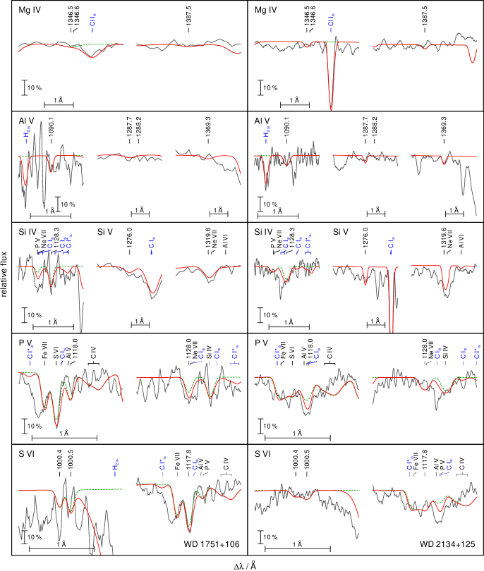
Figure 5: Like Fig. 3, for Mg iv, Al v, Si iv-v, P v, and S vi.

Aluminum.

Al V $\lambda\lambda\,1090.1,1287.7,1288.2,1369.3$ Å are the most prominent Al lines in the synthetic spectra (Fig. 5). We determined an abundance of $[\mathrm{Al}]={\color[rgb]{0,0,0}0.6}$ for WD 2134+125 an upper limit of $[\mathrm{Al}]<{\color[rgb]{0,0,0}0.7}$ for WD 1751+106.

Silicon.

In the STIS and GHRS observations of both stars, the Si IV $\lambda\lambda\,1393.8,1402.8$ Å resonance doublet is blended by interstellar absorption lines. Thus, our abundance determination is based on Si IV $\lambda\,1128.3$ Å and Si v $\lambda\lambda\,1118.8$, $1251.4$, $1276.0$, $1291.4$, $1319.6$ Å (Fig. 5). These lines indicate $[\mathrm{Si}]={\color[rgb]{0,0,0}-0.6}$ for WD 1751+106. For WD 2134+125, we used the same lines as well as Si V $\lambda\lambda\,1465.5,1582.7$ Å and measured $[\mathrm{Si}]={\color[rgb]{0,0,0}-0.7}$.

Phosphorus.

We used the strongest P lines, namely P V $\lambda\lambda\,1118.0,1128.0$ Å, in the theoretical spectra to establish upper limits of $[\mathrm{P}]<{\color[rgb]{0,0,0}0.3}$ for WD 1751+106 and $[\mathrm{P}]<{\color[rgb]{0,0,0}0.4}$ for WD 2134+125 (Fig. 5).

Sulfur.

The most prominent S lines in the FUSE spectrum of WD 1751+106 and WD 2134+125, S vi $\lambda\lambda\,933.4$, $944.5$ Å are both blended by interstellar $\mathrm{H}_{2}$ lines and thus it is uncertain to derive the S abundance. From S vi $\lambda\lambda\,1000.4$, $1000.5$, $1117.8$ Å (Fig. 5), we determine $[\mathrm{S}]={\color[rgb]{0,0,0}-0.1}$ and $[\mathrm{S}]\leq{\color[rgb]{0,0,0}-0.6}$ for WD 1751+106 and WD 2134+125, respectively.

Chlorine.

Cl VII $\lambda\lambda\,949.0,949.1,996.7,997.0$ Å are present in the synthetic spectra but cannot be identified in the FUSE observations of both stars. Based on these lines, we determined upper limits of $[\mathrm{Cl}]<{\color[rgb]{0,0,0}1.1}$ and $[\mathrm{Cl}]<{\color[rgb]{0,0,0}1.0}$ for WD 1751+106 and WD 2134+125, respectively.

Argon.

The strong Ar VII $\lambda\,1063.6$ Å line is blended by interstellar absorption and thus can not be used to derive an abundance value for argon. We used Ar VIII $\lambda\,1164.1$ Å to derive an upper limit of $[\mathrm{Ar}]<{\color[rgb]{0,0,0}0.3}$ for WD 1751+106 and $[\mathrm{Ar}]<{\color[rgb]{0,0,0}-0.3}$ for WD 2134+125 (Fig.6).

Calcium.

The strongest line in the synthetic spectra, namely Ca IX $\lambda\,1116.0$ Å, is blended with a strong interstellar $\mathrm{H}_{2}$ absorption feature. For WD 1751+106, this line appears in the wing of the $\mathrm{H}_{2}$ line and is used to derive an upper limit of $[\mathrm{Ca}]<{\color[rgb]{0,0,0}0.0}$.

Chromium.

None of the Cr VII lines appearing in the synthetic spectrum has been identified in the observation. We used Cr VII $\lambda\lambda\,1170.1,1186.6,1187.3$ Å to determine upper limits of $[\mathrm{Cr}]<{\color[rgb]{0,0,0}2.0}$ for WD 1751+106 and WD 2134+125.

Iron.

In previous analysis of NGC 7094, Miksa et al. (2002) found subsolar values of at least one dex for Fe. For the CS of Abell 43, they found a solar upper limit for Fe. With extended model atoms, Löbling (2018) checked and correct this result and determined $[\mathrm{Fe}]={\color[rgb]{0,0,0}-0.4}$ for WD 1751+106 and $[\mathrm{Fe}]={\color[rgb]{0,0,0}-0.8}$ for WD 2134+125. These values are supported also by our final model including all opacities of 31 elements (Fig. 7). Previous analyses that assumed a larger deficiency, did not take line broadening due to stellar rotation or macro turbulence into account explaining the lower Fe abundances. A solar Fe abundance can be ruled out since the computed lines of Fe VII appear too strong (Fig. 7)

Nickel.

The dominating ionization stages of the IGEs in the expected parameter regime are vii and viii. Due to the lack of POS lines of Ni in these stages in Kurucz’s line list (Kurucz 1991, 2009) for the spectral ranges of FUSE, STIS, and GHRS, no Ni lines could be detected and identified. In their analysis, Ziegler et al. (2009) used Ni VI lines and determined upper Ni abundance limits only. Their subsolar values may again be a result of not taking additional broadening due to rotation or macro turbulence into account. Furthermore, they assumed lower temperatures and higher gravities for both stars. The Ni VI lines are very sensitive to $T_{\mathrm{eff}}$ and are significantly stronger for a model with $T_{\mathrm{eff}}$ reduced by 10 kK (Fig. 8).

No strong lines in the spectra of both stars were found from the elements Sc, Ti, V, Mn, Ni, and Co. Therefore, these elements were combined to a generic model atom (Rauch & Deetjen 2003). All IGEs were taken into account with solar abundances ratios normalized to the Fe abundance in the final model calculations.

Zinc.

The strong lines Zn V $\lambda\lambda\,1132.3,1123.7,1133.0,1133.1,$ $1133.3,1133.5,1174.3,1180.0$ Å appear in the synthetic spectra but could not be identified in the observations. Thus, we can only derive an upper limit of $[\mathrm{Zn}]<{\color[rgb]{0,0,0}1.0}$ for both stars.

Gallium.

We used the strongest line Ga VI $\lambda\,1006.9$ Å to determine an upper limit of $[\mathrm{Ga}]<{\color[rgb]{0,0,0}2.0}$ for WD 1751+106 and WD 2134+125.

Germanium.

Ge VI $\lambda\lambda\,920.5,926.8,988.2$ Å are partly blended by interstellar absorption features. The analysis yields an upper limit of $[\mathrm{Ge}]<{\color[rgb]{0,0,0}2.0}$ for both stars.

Krypton.

Kr VII $\lambda\lambda\,1166.9,1169.6,1195.6,1284.6$ Å are present in the models. We used these lines to measure an upper limit of $[\mathrm{Kr}]<{\color[rgb]{0,0,0}3.5}$ for both stars.

Zirconium.

By analyzing STIS observation of WD 2134+125 around the computed lines Zr vii $\lambda\lambda\,1233.6$, $1235.0$, $1376.6$ Å ,we derived an upper limit of $[\mathrm{Zr}]<{\color[rgb]{0,0,0}3.0}$. Due to the fact that these lines are located in the range of the lower-resolution GHRS observation of WD 1751+106, we were not able to derive a reasonable value for this star.

Tellurium.

We used Te VI $\lambda\,1071.4$ Å, the strongest computed line in the FUSE range, to ascertain $[\mathrm{Te}]\leq{\color[rgb]{0,0,0}4.0}$ for WD 1751+106 and $[\mathrm{Te}]\leq{\color[rgb]{0,0,0}3.5}$ for WD 2134+125.

Iodine.

The strongest computed lines I vi $\lambda\lambda\,911.2$, $915.4$, $919.2$ Å are useless for the abundance measurement, since they are blended by interstellar absorption. Based on I VI $\lambda\lambda\,1045.4,1120.3,1153.3$ Å, we derived upper limits of $[\mathrm{I}]<{\color[rgb]{0,0,0}4.6}$ and $[\mathrm{I}]<{\color[rgb]{0,0,0}5.0}$ for WD 1751+106 and WD 2134+125, respectively.

Xenon.

We used the strongest line Xe VII $\lambda\,995.5$ Å to determine an upper limit of $[\mathrm{Xe}]<{\color[rgb]{0,0,0}4.0}$ for WD 2134+125. The quality of the FUSE observation of WD 1751+106 around this line does not suffice to determine the Xe abundance.

Selenium, strontium, molybdenum, and barium.

Even if we increase the Se, Sr, Mo, and Ba abundances in the synthetic models to thousand times solar, no lines of these elements appear in the computed spectra.

In our final models, all TIEs are taken into account with solar abundance ratios normalized to the determined Fe abundance value. The temperature and density structure and the ionization fractions of all ions considered in the final model for WD 2134+125 are shown in Fig. 20.

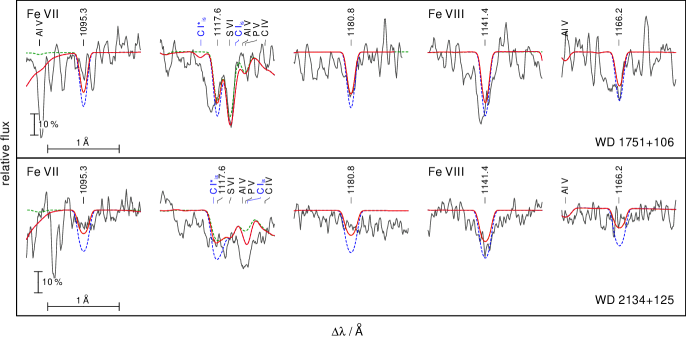
Figure 7: Synthetic spectra around Fe vii and viii lines calculated from our final models with $[\mathrm{Fe}]={\color[rgb]{0,0,0}-0.4}$ (red, full) and solar (blue, dashed) compared with the FUSE observation.

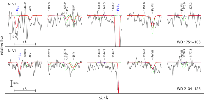
Figure 8: Top panel: Synthetic spectra around Ni vi lines calculated from our final models for WD 1751+106 with $\mbox{$T_{\mathrm{eff}}$}=115$ kK and $[\mathrm{Ni}]={\color[rgb]{0,0,0}-0.4}$ (red, full) and one dex supersolar (blue, dashed) and $\mbox{$T_{\mathrm{eff}}$}=105$ kK and Ni one dex supersolar (green, dotted). Bottom: For WD 2134+125 with $\mbox{$T_{\mathrm{eff}}$}=115$ kK and $[\mathrm{Ni}]={\color[rgb]{0,0,0}-0.8}$ (red, full) and one dex supersolar (blue, dashed) and $\mbox{$T_{\mathrm{eff}}$}=105$ kK and Ni one dex supersolar (green, dotted).

6 Stellar wind and mass loss

At $\mbox{$T_{\mathrm{eff}}$}=115\,000\,\mathrm{K}$ and $\log g=5.6$ the stars have luminosities of almost 4 000 $L_{\odot}$ (Sect. 7). They are located close to the Eddington limit and experience mass loss due to a radiation-driven wind (cf. Pauldrach et al. 1988) and, hence, exhibit prominent P Cygni profiles in their UV spectra (Fig. 9). Koesterke & Werner (1998) and Koesterke et al. (1998) investigated the wind properties of WD 2134+125 by means of NLTE models for spherically expanding atmospheres and determined the mass-loss rate $\dot{M}$ and the terminal wind velocity $v_{\infty}$ from HST/GHRS and ORFEUS-SPAS II observations, respectively. They found $\log[\dot{M}\,/\,(M_{\odot}/\mathrm{yr})]=-7.3$ from C IV $\lambda\lambda\,1548.20,1550.77$ Å and $\log[\dot{M}\,/\,(M_{\odot}/\mathrm{yr})]=-7.7$ from O VI $\lambda\lambda\,1031.91,1037.61$ Å and $v_{\infty}=3\,500\,\mathrm{km/s}$ which is slightly lower than the former value of $v_{\infty}=3\,900\,\mathrm{km/s}$ of Kaler & Feibelman (1985) based on the analysis of spectra obtained with IUE. Guerrero & De Marco (2013) used lines of O VI and found $3\,610\,\mathrm{km/s}$ for WD 2134+125 and $3\,000-3\,600\,\mathrm{km/s}$ from the analysis of O VI and Ne VII lines for WD 1751+106.
For the analysis of the wind lines in the UV range we used the PoWR model atmosphere code. This is a state-of-the-art NLTE code that accounts for mass- loss, line-blanketing, and wind clumping. It can be employed for a wide range of hot stars at arbitrary metallicities (e.g. Hainich et al. 2014, 2015; Reindl et al. 2014a; Oskinova et al. 2011; Shenar et al. 2015; Reindl et al. 2017), since the hydrostatic and wind regimes of the atmosphere are treated consistently (Sander et al. 2015). The NLTE radiative transfer is calculated in the co-moving frame. Any model can be specified by its luminosity $L$, stellar temperature $T_{\mathrm{eff}}$, surface gravity $g$, and mass-loss rate $\dot{M}$ as main parameters. In the subsonic region, the velocity field is defined such that a hydrostatic density stratification is approached (Sander et al. 2015). In the supersonic region, the wind velocity field $v(r)$ is pre-specified assuming the so-called $\beta$-law (Castor et al. 1975). Wind clumping is taken into account in first-order approximation (Hamann & Gräfener 2004) with a density contrast $D=\varrho_{\text{cl}}/\langle\varrho\rangle$ between the clumps and a smooth wind of same mass-loss rate. As we do not assume an interclump medium, $D=f_{V}^{-1}$.
We adopted the stellar parameters from the TMAP analysis as given in Table 3. Our calculations include complex model atoms for H, He, C, N, O, F, Ne, Si, P, S, and the iron group elements Sc, Ti, V, Cr, Mn, Fe, Co, Ni.
The only P Cygni line that is not saturated and is sensitive enough to the mass-loss rate is C IV $\lambda\lambda\,1548,1551$ Å. For WD 1751+106 the quality of the UV observation in this wavelength range is very poor. However, we found that the mass-loss rate must be $\log[\dot{M}\,/\,(M_{\odot}/\mathrm{yr})]\lesssim-8.1$ to obtain a model that is compatible with the observation. The STIS spectrum of WD 2134+125 in this wavelength range has a much better quality. We obtained the best fit to the complicated line profile of C IV $\lambda\lambda\,1548,1551$ Å by models with a mass-loss rate of $\log[\dot{M}\,/\,(M_{\odot}/\mathrm{yr})]\approx-8.1$. In both cases we assumed a density contrast of $D=10$, which is typically found for H-deficient CSPNe winds (Todt et al. 2008).
The blue edges of the P Cygni profiles of O VI $\lambda\lambda\,1032,1038$ Å and C IV $\lambda\lambda\,1548,1551$ Å were used to estimate the terminal wind velocity for WD 2134+125 of about $v_{\infty}=3300\pm 100\,$km/s and a $\beta=0.6$. Additional broadening due to depth dependent microturbulence with $v_{\text{D}}=20\,$km/s in the photosphere, estimated from, e.g., the F vi$\,\lambda 1140$ line, up to $v_{\text{D}}=230\,$km/s in the outer wind was taken into account and allows to fit the width of the O vi (Fig. 9) and the C iv resonance lines simultaneously. Similar values have been obtained for WD 1751+106, i.e. $v_{\infty}=3500\pm 100\,$km/s and $v_{\text{D}}=50\,$km/s in the photosphere up to $v_{\text{D}}=180\,$km/s in the outer wind. At these high mass-loss rates, the stellar wind is coupled and the photosphere is chemically homogeneous (Unglaub 2007, 2008).

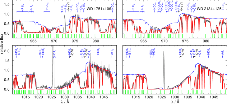
Figure 9: Comparison of synthetic spectra calculated with PoWR (blue line, dotted) compared with the FUSE observation of WD 1751+106 (left) and WD 2134+125 (right). In red a combined wind+ISM spectrum is shown. The wind models are calculated with a mass-loss rate of $\log[\dot{M}\,/\,(M_{\odot}/\mathrm{yr})]=-8.1$, and $v_{\infty}=3\,500\,\mathrm{km/s}$ for WD 1751+106 and $v_{\infty}=3\,300\,\mathrm{km/s}$ for WD 2134+125. Upper panel: around Ne vii $\lambda\,973.33$ Å, lower: around O vi $\lambda\lambda\,1031.91,1037.61$ Å. The green marks at the bottom of each panel indicate wavelengths of strong interstellar H₂ lines.

7 Mass, luminosity, and distance

The determination of the mass of WD 1751+106 and WD 2134+125 is difficult since their evolutionary history is not unambiguous. If they are AFTP stars no appropriate set of evolutionary tracks is available in the literature to compare with. Lawlor & MacDonald (2006) presented a variety of calculations for the evolution of H-deficient post-AGB stars. The so-called AGB departure type V scenario (departure from the AGB during a He flash) and the type IV scenario appear to be in the transition between AFTP and LTP (Table 1). A different H/He ratio should have an influence on the result (cf. Miller Bertolami & Althaus 2007). To decide which grid of post-AGB tracks should be used, we calculated some AFTP models with LPCODE (Althaus et al. 2003, 2005) (Table 1). This was done by recomputing the end of the AGB evolution of three models presented in Miller Bertolami (2016) and tuning the mass loss at the end of the AGB phase as to enforce an AFTP event. These sequences have $(M_{\rm ZAMS}$, $Z_{\rm ZAMS}$, $M_{\rm f})=$ $(1.25M_{\odot}$, $0.01$, $0.566M_{\odot})$, $(1.00M_{\odot}$, $0.001$, $0.550M_{\odot})$, $(1.50M_{\odot}$, $0.001$, $0.594M_{\odot})$ (Table 1). At the location of the stars in the $\log g$-$T_{\mathrm{eff}}$ diagram, the tracks for VLTP and AFTP stars coincide (Fig. 10). Thus, the approach of using VLTP tracks for the determination of the mass is acceptable.
We find $M=0.57^{+0.07}_{-0.04}\,M_{\odot}$ for WD 1751+106 and WD 2134+125. Using the initial-final mass relation of Cummings et al. (2018), these stars originate from progenitors with initial mass of about $1.0$ to $1.1\,M_{\odot}$. From the 0.515, 0,530, 0,542, 0,565, 0.584, 0.609, and 0.664$\,M_{\odot}$ tracks (Fig. 10), we determine the luminosity of $\log L\,/\,L_{\odot}=3.77^{+0.23}_{-0.24}$ for WD 1751+106 and WD 2134+125.
The spectroscopic distances are calculated following the flux calibration of Heber et al. (1984),

$$f_{\mathrm{V}}=3.58\times 10^{-9}\times 10^{{\rm-0.4}m_{\mathrm{V_{0}}}}\,\mathrm{erg\,cm^{-2}\,s^{-1}}\,{\text{\AA}}^{-1}$$ (1)

with $m_{\mathrm{V_{0}}}=m_{\mathrm{V}}-2.175c$, $c=1.47E_{\mathrm{B-V}}$. We take $m_{\mathrm{V}}=14.75\pm 0.13$ (Acker et al. 1992) and $c=0.390\pm 0.015$ using our determination of $E_{\mathrm{B-V}}$ for WD 1751+106 and $m_{\mathrm{V}}=13.68\pm 0.25$ (Acker et al. 1992) and $c=0.199\pm 0.015$ for WD 2134+125. The distance is derived from

$$d\,/\,pc=7.11\times 10^{4}\sqrt{H_{\nu}(M/M_{\odot})\times 10^{(0.4m_{\mathrm{V_{0}}}-\log g)}}\,.$$ (2)

The Eddington flux at $\lambda_{\mathrm{eff}}=5454\,{\text{\AA}}$ of our final model atmospheres including all 31 elements is $H_{\nu}=(1.89\pm 0.19)\times 10^{-3}\mathrm{erg\,cm^{-2}\,s^{-1}\,Hz^{-1}}$ for WD 1751+106 and $H_{\nu}=(1.88\pm 0.20)\times 10^{-3}\mathrm{erg\,cm^{-2}\,s^{-1}\,Hz^{-1}}$ for WD 2134+125. We derive distances of $d=2.23^{+0.31}_{-0.33}\,\mathrm{kpc}$ for WD 1751+106 and $d=1.65^{+0.32}_{-0.31}\,\mathrm{kpc}$ for WD 2134+125. WD 1751+106 is located $0.67^{+0.10}_{-0.10}\,\mathrm{kpc}$ above the Galactic plane and WD 2134+125 has a depth below the Galactic plane of $0.78^{+0.15}_{-0.15}\,\mathrm{kpc}$. Taking into account the angular sizes of the nebulae measured from narrow-band images by Rauch (1999), the nebula shells of Abell 43 and NGC 7094 have radii of $R=0.48^{+0.07}_{-0.07}\,\mathrm{pc}$ and $R=0.42^{+0.08}_{-0.08}\,\mathrm{pc}$, respectively. With the measured expansion velocity of $40\pm 2\,\mathrm{km/s}$ for Abell 43 and $38\pm 2\,\mathrm{km/s}$ for NGC 7094 (Pereyra et al. 2013), the expansion times are $11\,600^{+1\,600}_{-1\,700}\,\mathrm{yrs}$ and $10\,900^{+2\,100}_{-2\,000}\,\mathrm{yrs}$, respectively. These dynamical timescales place a lower limit to the actual age of the PNe since velocity gradients and the acceleration over time are not taken into account (Gesicki & Zijlstra 2000). Dopita et al. (1996) derived typical correction factors of 1.5. Both stars are targets of the Gaia mission and contained in the data made public in the second data release (DR2). Gaia measured parallaxes of $0\aas@@fstack{\prime\prime}431\pm 0\aas@@fstack{\prime\prime}061$ and $0\aas@@fstack{\prime\prime}615\pm 0\aas@@fstack{\prime\prime}059$ (Gaia Collaboration 2018) for WD 1751+106 (ID 4488953930631143168) and WD 2134+125 (ID 1770058865674512896), respectively. This corresponds to relative errors of $14.1\,\%$ and $9.5\,\%$. From these values, Bailer-Jones et al. (2018) derived distances of $2.19^{+0.35}_{-0.27}\,$ kpc for WD 1751+106 and $1.55^{+0.16}_{-0.13}$ kpc for WD 2134+125. These values are in good agreement with our spectroscopic distance determination and validate the mass determination by spectroscopic means using stellar atmosphere models and evolutionary tracks.

Table 1: Photospheric abundances of WD 1751+106 and WD 2134+125 compared with evolutionary models.

$T_{\mathrm{eff}}$		H		He		C		N		O		Ne
	$\log(g\,/\,\textrm{cm}/\textrm{s}^{2})$													comment
(K)		(mass fraction)
115 000	5.6	0.	15	0.	52	0.	31	0.	0003	0.	0033	0.	0019	WD 2134+125, our atmosphere model
115 000	5.6	0.	25	0.	46	0.	27	0.	0026	0.	0044	0.	012	WD 1751+106, our atmosphere model
84 000	5.0	0.	444	0.	539	0.	012	0.	002	0.	002	0.	0008	Lawlor & MacDonald (2006, AGB departure type IV)
140 000	6.0	0.	106	0.	794	0.	085	0.	002	0.	012	0.	003	Lawlor & MacDonald (2006, AGB departure type IV)
87 000	5.0	0.	565	0.	427	0.	005	0.	0009	0.	0009	0.	0004	Lawlor & MacDonald (2006, AGB departure type V)
150 000	6.0	0.	164	0.	775	0.	051	0.	0014	0.	0057	0.	002	Lawlor & MacDonald (2006, AGB departure type V)
		0.	197	0.	450	0.	296	0.	0001	0.	056	0.	00078	AFTP model $M_{\mathrm{f}}=0.550$, $Z=0.001$
		0.	137	0.	390	0.	357	0.	0006	0.	104	0.	0085	AFTP model $M_{\mathrm{f}}=0.566$, $Z=0.01$
		0.	219	0.	445	0.	258	0.	0007	0.	055	0.	021	AFTP model $M_{\mathrm{f}}=0.594$, $Z=0.001$

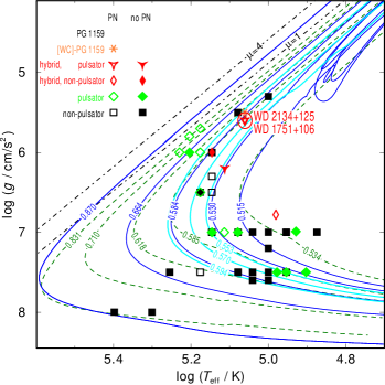
Figure 10: Positions of WD 1751+106 (Abell 43) and WD 2134+125 (NGC 7094) with their error ellipses and related objects in the $\log\mbox{$T_{\mathrm{eff}}$}-\mbox{$\log g$}$ plane compared with evolutionary tracks (labeled with the respective masses in M_⊙) of VLTP stars (Miller Bertolami & Althaus 2006, blue full lines), of H-burning post-AGB stars (calculated with initial solar metallicity, Miller Bertolami 2016, green dashed lines), and of AFTP stars (cyan, thick lines).The dashed-dotted $\mu=1$ and $\mu=4$ lines indicate the Eddington limits for pure H and He atmospheres, respectively.

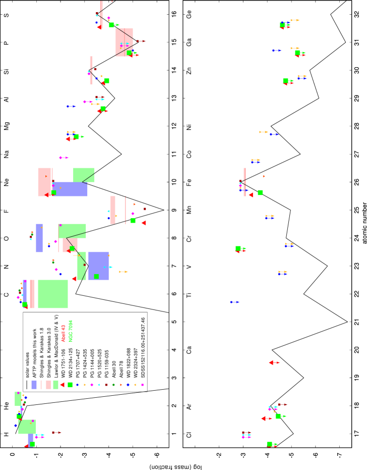
Figure 11: Photospheric abundances for a set of PG 1195 stars and calculated ranges from evolutionary models. For the models of Shingles & Karakas (2013), the initial mass of the star in $M_{\odot}$ is given in the legend box. Upper limits are indicated with arrows. The solid black lines indicates solar abundances.

8 Discussion

Our aim was to determine the element abundances of WD 1751+106 and WD 2134+125 beyond He and H. The results are shown in Table 3. By comparing our results to the abundances of other post-AGB stars and evolutionary models, we are able to conclude constraints for nucleosynthesis processes and evolutionary channels. The H-deficient nature of WD 1751+106 and WD 2134+125 suggests that here, as in other H-deficient stars, we see nuclear processed material on the surface that has formed either during the progenitor AGB phase or the same mixing and burning processes that lead to the H-deficiency in the first place. Figure 11 illustrates the following sections.

8.1 Comparison to other hybrid PG 1159 stars

The group of known hybrid PG 1159 stars comprises the CS of Sh 2$-$68 and HS 2324+3944 (WD 1822+008 and WD 2324+397, respectively, McCook & Sion 1999a, b) and SDSS 152116.00+251437.46 (Werner & Herwig 2006; Werner et al. 2014), besides the two program stars of this work. The known atmospheric parameters for these objects are summarized in Table 2. For WD 1822+008, Gianninas et al. (2010) found $T_{\mathrm{eff}}=84\,460$ K and $\log g=7.24$. Its position in the $\log T_{\mathrm{eff}}$-$\log g$ diagram (Fig. 10) suggests that the star is already located close to the beginning of the WD cooling track and is thus further evolved than the two stars of this work. The large distance of $1000\pm 400$ pc (Binnendijk 1952) was reduced and better constrained to $399.7^{+11.8}_{-12.5}$ pc (Bailer-Jones et al. 2018) using Gaia data. With its a diameter of $400^{\prime\prime}\pm 70^{\prime\prime}$ (Fesen et al. 1983), the PN has a radius of $0.388^{+0.082}_{-0.078}$ pc. Considering an expansion velocity of $7.5$ km/s (Hippelein & Weinberger 1990), this yields a dynamic timescale of $50\,600^{+10\,700}_{-10\,200}$ yrs which confirms the suggestion from the location in the $\log T_{\mathrm{eff}}$-$\log g$ diagram and assigns Sh 2$-$68 to the group of oldest and largest PNe. It has a lower element ratio of He/H compared to WD 1751+106 and WD 2134+125. This might result from ongoing depletion of heavier elements from the atmosphere due to gravitational settling.
WD 2324+397 ($T_{\mathrm{eff}}=130\,000\pm 10\,000$ K and $\log g=6.2\pm 0.2$, Dreizler et al. 1996) and SDSS 152116.00+251437.46 ($T_{\mathrm{eff}}=140\,000\pm 15\,000$ K and $\log g=6.0\pm 0.3$, Werner et al. 2014) are members of this group without an ambient PN (Werner et al. 1997). The C abundance is similar to the values determined for our two program stars. Considering the C/H ratio, the value for SDSS 152116.00+251437.46 is close to the one of WD 2134+125 while the one for WD 2324+397 is slightly higher. Both their O/H ratios exceeds the values of our two program stars by a factor of two or even more. The N/H ratio of the stars for which it is known is very low. The He/H ratio of WD 2324+397 resembles the value of WD 1751+106 whereas WD 2134+125 has a higher He content similar to SDSS 152116.00+251437.46.

Table 2: Photospheric abundances of WD 1751+106 and WD 2134+125 compared with other hybrid PG 1159 stars and the CSPNe Abell 30 and Abell 78.

	$T_{\mathrm{eff}}$			H		He		C		N		O
Object		$\log(g\,/\,\textrm{cm}/\textrm{s}^{2})$												Reference
	(K)			(mass fraction)
WD 2134+125	115 000	5.	6	0.	15	0.	52	0.	31	0.	0003	0.	0032	this work
WD 1751+106	115 000	5.	6	0.	25	0.	46	0.	27	0.	0026	0.	0044	this work
WD 1822$+$008	84 460	7.	24	0.	66	0.	34							Gianninas et al. (2010)
WD 2324$+$397	130 000	6.	2	0.	17	0.	35	0.	42	0.	0001	0.	06	Dreizler et al. (1996); Dreizler (1999)
SDSS 152116.00+251437.46	140 000	6.	0	0.	14	0.	56	0.	29			0.	01	Werner et al. (2014)
Abell 30	115 000	5.	5			0.	41	0.	40	0.	04	0.	15	Leuenhagen et al. (1993)
Abell 78	117 000	5.	5			0.	30	0.	50	0.	02	0.	15	Toalá et al. (2015); Werner & Koesterke (1992)

8.2 Comparison to Abell 30 and Abell 78

Comparing the results of our analysis to the parameters known for the CSs of the PNe Abell 30 and Abell 78 is of special interest, because these objects are located at almost the same position in the $\log T_{\mathrm{eff}}$-$\log g$ diagram. Both are [WC]-PG 1159 transition objects with $T_{\mathrm{eff}}=115\,000$ K and $\log g=5.5$ (Leuenhagen et al. 1993) and $T_{\mathrm{eff}}=117\,000\pm 5000$ K and $\log g=5.5$ (Toalá et al. 2015; Werner & Koesterke 1992). Their element mass fractions are also included in Table 2. Obvious are the higher He and lower C, N, and O abundances in our two hybrid PG 1159 stars. This may result from different evolutionary channels. The CSs of Abell 30 and Abell 78 both underwent a born-again scenario (Iben et al. 1983) resulting in a return to the AGB, whereas the hybrid PG 1159 stars experience a final He-shell flash at the departure from the AGB. This AFTP evolution may be the reason for the smaller amount of C, N, and O in the atmosphere in contrast to a (V)LTP scenario. Toalá et al. (2015) found a Fe deficiency of about one dex for Abell 78. This subsolar Fe abundance is in good agreement with the results for WD 1751+106 and WD 2134+125, although they show a smaller Fe deficiency. The high Ne abundance of $4$ % by mass of the CS of Abell 78 (Toalá et al. 2015) and the revised N abundance of $1.5$ % by mass for both CSPNe (Guerrero et al. 2012; Toalá et al. 2015) exceed the values determined for out two hybrid stars and are also an indicator for different evolutionary channels, namely VLTP and AFTP evolution. In common with the CS of Abell 78 is the high abundance of F ($25$ times solar, Toalá et al. 2015) compared to $9.3$ and $29$ times solar, for WD 1751+106 and WD 2134+125 respectively). Their mass loss rates of $\dot{M}/M_{\odot}=2.0\times 10^{-8}\,\mathrm{yr}^{-1}$ (Guerrero et al. 2012) and $\dot{M}/M_{\odot}=1.6\times 10^{-8}\,\mathrm{yr}^{-1}$ (Toalá et al. 2015) are about a factor two higher than the ones determined for WD 1751+106 and WD 2134+125 (Sect. 6). The PNe Abell 30 and Abell 78 look very similar in shape but appear different to the “Galactic Soccerballs”.

8.3 Comparison to PG 1159 stars, hot post-AGB stars, and nucleosynthesis models

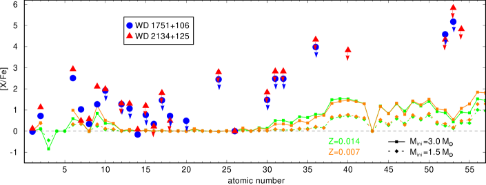
Figure 12: Photospheric abundance ratio $[\mathrm{X}/\mathrm{Fe}]=\log(n_{\mathrm{X}}/n_{\mathrm{Fe}})-\log(n_{\mathrm{X},\odot}/n_{\mathrm{Fe},\odot})$ with the number fraction $n_{\mathrm{X}}$ for element X of WD 1751+106 and WD 2134+125 determined from detailed line-profile fits. Upper limits are indicated with arrows. Predictions of Karakas & Lugaro (2016, $M_{\mathrm{ini}}=1.5$ and $3.0$ (see legend); metallicity $Z=0.014$ (green) and $0.007$ (cyan)) are shown for comparison.

Karakas & Lugaro (2016) presented a grid of evolutionary models for different initial masses and metallicities. For stars with initial masses $M\leq 3\,M_{\odot}$, they predict an enhanced production of C, N, F, Ne, and Na compared to solar values and normalized to the value for Fe. This prediction for the surface abundances of post-AGB stars is in line with our abundance determinations (Fig. 12). Another set of evolutionary models for initial masses of $1.8-6\,M_{\odot}$ was calculated by Shingles & Karakas (2013) to investigate the resulting element yields of the species He, C, O, F, Ne, Si, P, S, and Fe depending on uncertainties in nucleosynthesis processes. They present the intershell abundances of their stellar models that should represent the surface abundances of PG 1159 stars. As described in (Sect. 1), the surface abundances of hybrid PG 1159 stars should reflect a mixture of the abundances of the former H-rich envelope and the intershell.
The C abundances of our two program stars resemble the values of other PG 1159 stars like for example the prototype star PG 1159$-$035 (Jahn et al. 2007), the hot PG 1159 stars PG 1520+525 and PG 1144+005 (Werner et al. 2016) and the “cooler” PG 1707+427 and PG 1424+535 (Werner et al. 2015).
The subsolar O abundances of the two stars analyzed in this work are significantly lower than the supersolar values of the stars mentioned above. However, the O abundance of the hybrid PG 1159 stars lie within the predicted range of Shingles & Karakas (2013) (O mass fraction between 0.2 and 1.2 %) and Lawlor & MacDonald (2006) in comparison to the PG 1159 stars. The large range in O abundances may be caused by different effectiveness of convective boundary mixing of the pulse-driven convection zone into the C/O core in the thermal pulses on the AGB.
An N enrichment is predicted for PG 1159 stars that experienced a VLTP scenario due to a large production of ¹⁴N in an H-ingestion flash (HIF, cf., Werner & Herwig 2006). WD 1751+106 and WD 2134+125 experienced an AFTP without HIF what corresponds to their comparatively low N abundance. The value for WD 2134+125 lies within the range that is predicted by AFTP models whereas the value for WD 1751+106 is higher.
The set of PG 1159 stars shows a large range of F abundances from low mass fractions of $3.2\times 10^{-6}$ for the prototype PG 1159$-$035 to values of $1.0\times 10^{-4}$ for PG 1707$-$427. The values of WD 1751+106 and WD 2134+125 lie within this range but below the predictions of Shingles & Karakas (2013) (F mass fractions between $2.0\times 10^{-5}$ and $2.7\times 10^{-4}$). The F production in the intershell region is very sensitive on the temperature and therefore on the initial mass (Lugaro et al. 2004). They predict the highest F abundances for stars with initial masses of $2-4\,M_{\odot}$ at solar metallicity (F intershell mass fractions of $3-7\times 10^{-5}$). Again, the values of WD 2134+125 and WD 1751+106 are about 3 to 10 times lower than these predictions.
The Ne abundances for the set of mentioned PG 1159 stars are all supersolar and in agreement with evolutionary models. The determined values for the Si, P, and S abundances are at the lower border or slightly below the predictions from evolutionary models. The same holds for the solar upper abundance limit for P in PG 1159$-$035.
The Fe deficiency is are not explained by nucleosynthesis calculations like those of Karakas & Lugaro (2016) that predict solar Fe abundances for stars with a initial solar composition, which is due to the fact that iron is not strongly depleted in nuclear processes in AGB stars with masses ranging from $0.8-8.0\,M_{\odot}$ as it is the case for the precursor AGB stars of Abell 43 and NGC 7094. The models of Shingles & Karakas (2013) yield a slightly subsolar Fe abundances but still cannot explain the observed deficiency. For some of the PG 1159 stars of the set used for comparison here, the Fe abundance has been measured and all are found to be solar. The only other star in Fig. 11 which, besides WD 1751+106 and WD 2134+125, shows a Fe deficiency is the CSPN of Abell 78 (Sect. 8.2). The Fe deficiency of 0.4 and 0.8 dex for WD 1751+106 and WD 2134+125, respectively, does not include solar values within the error ranges. Löbling (2018) discuss the speculation of Herwig et al. (2003) that this underabundance can be caused by neutron capture during the former AGB phase leading to a transformation of Fe into Ni and heavier elements. Probably the low Fe abundances determined in WD 1751+106 and WD 2134+125 are just a consequence of a low initial metal content for these objects. This subsolar metallicity does not rule out a thick or even thin disc membership (Recio-Blanco et al. 2014). Also their location and distance to the Galactic plane support that these are disc objects. The models of Karakas & Lugaro (2016) predict a strong enhancement of the TIEs in the atmospheres of post-AGB stars. Unfortunately, no abundance determination was possible for the TIEs but due to the determined upper abundance limits for Zn, Ga, Ge, Kr, and Te of both stars and Zr for WD 2134+125 a strong enhancement can be ruled out. This is consistent with our determination of the wind intensity for which the wind is coupled. Thus, this prevents diffusion and disrupts the equilibrium balance between radiative levitation and gravitational settling. To improve the analysis of TIEs, spectra with much better S/N and the calculation of reliable atomic data are highly desirable.

9 Conclusion

Regarding the evolutionary scenario for WD 1751+106 and WD 2134+125, an AFTP remains the best available candidate. The AFTP models presented here (Fig. 10 and Table 1) are able to reproduce qualitatively the observed trends. Abundances of H, He, C, N, and Ne are reasonably well reproduced by AFTP models. However AFTP models computed from sequences that include convective boundary mixing at the bottom of the pulse driven convective zone (as those presented here) display O abundances much larger than those of our program stars. In fact, the O abundances shown by our stars are in good agreement with those predicted by Lawlor & MacDonald (2006), using AGB models that do not include any type of convective boundary mixing at the bottom of the pulse driven convective zone. These models, however, underestimate the C and Ne abundance, while the H and He abundances reproduce the observed values. Yet, the main argument against the AFTP scenario comes from the expansion ages of the nebulae. According to stellar evolution computations, AFTP models reach the location of our program stars in the HRD less than 2000 yr after departing from the AGB, while the expansion ages are several times larger than this. This is true regardless the mass-loss prescription adopted in the post-AGB evolution. Unless the masses of the CSPNe are much lower than derived here, the AFTP scenario is unable to reproduce this key observational feature.
It is desirable to determine the iron abundance and the abundances of heavier elements of the ambient PN to investigate on the photospheric composition of Abell 43 and NGC 7094 at the time of the PN’s ejection and to analyze the elements produced and ejected during the preceding AGB phase (cf., Lugaro et al. 2017) but this is out of the focus of this paper.

Table 3: Parameters of WD 1751+106 and WD 2134+125 compared with literature values.

	WD 1751+106				WD 2134+125
	Literature		This work		Literature		This work
$T_{\mathrm{eff}}$ / kK	$115\pm 5$ a		$115\pm 5$		$115\pm 5$ a		$115\pm 5$
$\log\,(g$ / cm/s2)	$5.5\pm 0.1$ a		$5.6\pm 0.1$		$5.4\pm 0.1$ a		$5.6\pm 0.1$
$E_{\mathrm{B-V}}$	$0.265\pm 0.035$ e		$0.265\pm 0.010$		$0.150\pm 0.040$ d		$0.135\pm 0.010$
$N_{\text{H\,{i}}}$ / cm-2	$(1.0\pm 0.2)\times 10^{21}$ e		$(1.0\pm 0.1)\times 10^{21}$		$(7.0\pm 0.1)\times 10^{20}$ d		$(6.5\pm 0.1)\times 10^{20}$
$v_{\mathrm{rad}}$ / km/s	$-42.0\pm 11.5$ c		$-100\pm 10$		$-101.1\pm 30.8$ c		$-53\pm 10$
$d$ / kpc	$2.47\pm 0.30$ f		$2.23^{+0.31}_{-0.33}$		$1.75\pm 0.36$ f		$1.65^{+0.32}_{-0.31}$
$M\,/\,M_{\odot}$	$0.53^{+0.10}_{-0.02}$ e		$0.57^{+0.07}_{-0.04}$		$0.53^{+0.06}_{-0.06}$ d		$0.57^{+0.07}_{-0.04}$
$\log\ (L\,/\,L_{\odot})$	$3.44^{+0.50}_{-0.58}$ e		$3.77^{+0.23}_{-0.24}$				$3.77^{+0.23}_{-0.24}$
$R_{\mathrm{PN}}$ / pc	$0.51$ h		$0.48^{+0.07}_{-0.07}$		$0.51$ h		$0.42^{+0.08}_{-0.08}$

Notes. ^(a)Löbling (2018), ^(b)Ziegler et al. (2009), ^(c)Durand et al. (1998), ^(d)Ziegler (2008), ^(e)Friederich (2010), ^(f)Frew et al. (2016), ^(g)Ringat et al. (2011), ^(h)Napiwotzki (1999)

Table 3: Continued.

	WD 1751+106								WD 2134+125
	Literature			This work					Literature			This work
Abundances	[X]	Mass fraction		[X]	Mass fraction	Number fraction	[X/Fe]		[X]	Mass fraction		[X]	Mass fraction	Number fraction	[X/Fe]
H	$-$ 0.483 g	$2.43\times 10^{-1}$		$-$ 0.5	$2.5\times 10^{-1}$	$6.4\times 10^{-1}$	$-$0.0		$-$ 0.62 b	$1.77\times 10^{-1}$		$-$ 0.7	$1.5\times 10^{-1}$	$4.9\times 10^{-1}$	0.1
He	0.350 g	$5.59\times 10^{-1}$		0.3	$4.6\times 10^{-1}$	$3.0\times 10^{-1}$	0.7		0.45 b	$7.03\times 10^{-1}$		0.3	$5.2\times 10^{-1}$	$4.3\times 10^{-1}$	1.1
C	1.909 g	$1.75\times 10^{-1}$		2.1	$2.7\times 10^{-1}$	$5.8\times 10^{-2}$	2.5		1.76 b	$1.24\times 10^{-1}$		2.1	$3.1\times 10^{-1}$	$8.4\times 10^{-2}$	2.9
N	$-$ 0.491 g	$2.00\times 10^{-4}$		0.6	$2.6\times 10^{-3}$	$4.8\times 10^{-4}$	1.0		$-$ 0.85 b	$8.73\times 10^{-5}$		$-$ 0.3	$3.3\times 10^{-4}$	$7.7\times 10^{-5}$	0.5
O	$-$ 0.516 g	$1.63\times 10^{-3}$		$-$ 0.1	$4.4\times 10^{-3}$	$7.2\times 10^{-4}$	0.3		$-$ 1.81 b	$8.20\times 10^{-5}$		$-$ 0.2	$3.2\times 10^{-3}$	$6.7\times 10^{-4}$	0.6
F	0.694 g	$2.50\times 10^{-6}$		1.0	$3.3\times 10^{-6}$	$4.5\times 10^{-7}$	1.3		0.34 b	$1.11\times 10^{-6}$		1.5	$9.9\times 10^{-6}$	$1.7\times 10^{-6}$	2.1
Ne				$\leq$ 1.5	$\leq 3.6\times 10^{-2}$	$\leq 4.7\times 10^{-3}$	$\leq$ 1.9		0.00 b	$1.02\times 10^{-3}$		1.2	$1.9\times 10^{-3}$	$3.1\times 10^{-3}$	2.0
Mg	$\leq$ 0.108 e	$\leq$ $7.74\times 10^{-4}$		$\leq$ 0.8	$\leq 4.7\times 10^{-3}$	$\leq 5.0\times 10^{-4}$	$\leq$1.3					$\leq$ 0.5	$\leq 2.2\times 10^{-3}$	$\leq 3.0\times 10^{-4}$	$\leq$ 1.3
Al	$\leq$ 0.797 e	$\leq$ $2.90\times 10^{-4}$		$\leq$ 0.6	$\leq 2.3\times 10^{-4}$	$\leq 2.2\times 10^{-5}$	$\leq$1.1					0.5	$1.7\times 10^{-4}$	$2.1\times 10^{-5}$	1.3
Si	$-$ 0.560 g	$1.83\times 10^{-4}$		$-$ 0.6	$1.6\times 10^{-4}$	$1.5\times 10^{-5}$	$-$0.2		$-$ 0.21 b	$4.10\times 10^{-4}$		$-$ 0.7	$1.2\times 10^{-4}$	$1.4\times 10^{-5}$	0.1
P	$-$ 0.593 g	$1.33\times 10^{-6}$		$\leq$ 0.3	$\leq 1.2\times 10^{-5}$	$\leq 1.0\times 10^{-6}$	$\leq$0.8		$-$ 1.15 b	$3.70\times 10^{-7}$		$\leq$ 0.4	$\leq 1.4\times 10^{-5}$	$\leq 1.5\times 10^{-6}$	$\leq$ 1.2
S	$-$ 0.378 g	$1.36\times 10^{-4}$		$-$ 0.1	$2.4\times 10^{-4}$	$1.9\times 10^{-5}$	0.3		0.16 b	$4.69\times 10^{-4}$		$\leq-$ 0.6	$\leq 7.8\times 10^{-5}$	$\leq 8.0\times 10^{-6}$	$\leq$ 0.2
Cl				$\leq$ 1.0	$\leq 8.3\times 10^{-5}$	$\leq 6.1\times 10^{-6}$	$\leq$ 1.5					$\leq$ 1.0	$\leq 8.1\times 10^{-5}$	$\leq 7.5\times 10^{-6}$	$\leq$ 1.8
Ar	$\leq$ 1.307 e	$\leq$ $1.04\times 10^{-3}$		$\leq$ 0.3	$\leq 1.4\times 10^{-4}$	$\leq 8.8\times 10^{-6}$	$\leq$0.7		0.00 d	$4.43\times 10^{-5}$		$\leq-$ 0.3	$\leq 3.5\times 10^{-5}$	$\leq 2.9\times 10^{-6}$	$\leq$ 0.5
Ca				$\leq$ 0.0	$\leq 6.5\times 10^{-5}$	$\leq 4.5\times 10^{-6}$	$\leq$ 0.5
Cr				$\leq$ 2.0	$\leq 1.7\times 10^{-3}$	$\leq 8.1\times 10^{-5}$	$\leq$ 2.5					$\leq$ 2.0	$\leq 1.6\times 10^{-3}$	$\leq 1.0\times 10^{-4}$	$\leq$ 2.8
Fe	$-$ 0.691 e	$2.35\times 10^{-4}$		$-$ 0.4	$4.5\times 10^{-4}$	$2.1\times 10^{-5}$	0.0		$\leq-$ 1.00 b	$\leq$ $1.15\times 10^{-4}$		$-$ 0.8	$2.0\times 10^{-4}$	$1.2\times 10^{-5}$	0.0
Ni	$\leq-$ 1.000 e	$\leq$ $7.30\times 10^{-6}$							$\leq-$ 1.00 b	$\leq$ $7.30\times 10^{-6}$
Zn				$\leq$ 1.0	$\leq 1.7\times 10^{-5}$	$\leq 7.2\times 10^{-7}$	$\leq$1.5					$\leq$ 1.0	$\leq 1.7\times 10^{-5}$	$\leq 9.1\times 10^{-7}$	$\leq$ 1.8
Ga				$\leq$ 2.0	$\leq 5.6\times 10^{-6}$	$\leq 2.2\times 10^{-7}$	$\leq$2.5					$\leq$ 2.0	$\leq 5.6\times 10^{-6}$	$\leq 2.8\times 10^{-7}$	$\leq$ 2.8
Ge				$\leq$ 2.0	$\leq 2.4\times 10^{-5}$	$\leq 8.9\times 10^{-7}$	$\leq$2.5					$\leq$ 2.0	$\leq 2.4\times 10^{-5}$	$\leq 1.1\times 10^{-6}$	$\leq$ 2.8
Kr				$\leq$ 3.5	$\leq 3.4\times 10^{-4}$	$\leq 1.1\times 10^{-5}$	$\leq$4.0					$\leq$ 3.5	$\leq 3.4\times 10^{-4}$	$\leq 1.4\times 10^{-5}$	$\leq$ 4.3
Zr												$\leq$ 3.0	$\leq 2.5\times 10^{-5}$	$\leq 9.6\times 10^{-7}$	$\leq$ 3.8
Te				$\leq$ 4.0	$\leq 1.4\times 10^{-4}$	$\leq 3.8\times 10^{-6}$	$\leq$4.6					$\leq$ 3.5	$\leq 4.5\times 10^{-5}$	$\leq 1.2\times 10^{-6}$	$\leq$ 4.3
I				$\leq$ 4.6	$\leq 1.3\times 10^{-4}$	$\leq 3.6\times 10^{-6}$	$\leq$5.2					$\leq$ 5.0	$\leq 3.3\times 10^{-4}$	$\leq 8.9\times 10^{-6}$	$\leq$ 5.8
Xe												$\leq$ 4.0	$\leq 1.7\times 10^{-4}$	$\leq 4.4\times 10^{-6}$	$\leq$ 4.8

Notes. [X] = log (abundance/solar abundance), $[\mathrm{X}/\mathrm{Fe}]=\log(n_{\mathrm{X}}/n_{\mathrm{Fe}})-\log(n_{\mathrm{X},\odot}/n_{\mathrm{Fe},\odot})$ with the number fraction $n_{\mathrm{X}}$ for element X, the error of our abundance determination is $\pm 0.3$ dex, ^(a)Löbling (2018), ^(b)Ziegler et al. (2009), ^(c)Durand et al. (1998), ^(d)Ziegler (2008), ^(e)Friederich (2010), ^(f)Frew et al. (2016), ^(g)Ringat et al. (2011), ^(h)Napiwotzki (1999)

Appendix A Additional figures and tables.

Table 4: Statistics of the H – Ar^a and Ca - Ba^b model atoms used in our model-atmosphere calculations.

		Levels						Super	Super	Individual
Ion				Lines		Ion
		NLTE	LTE					levelsc	lines	lines
H	I	10	22	45		Ca	VII	7	27	71 608
	II	1	0	$-$			VIII	7	26	9 124
He	I	5	98	3			IX	1	0	0
	II	16	16	120		Cr	VII	7	24	37 070
	III	1	0	$-$			VIII	7	25	132 221
C	III	1	104	0			IX	1	0	0
	IV	54	4	295		Fe	VII	7	24	200 455
	V	1	0	0			VIII	7	27	19 587
N	IV	1	93	0			IX	1	0	0
	V	54	8	297		IGd	VII	7	27	5 216 215
	VI	1	0	0			VIII	7	28	2 218 561
O	V	10	124	14			IX	1	0	0
	VI	54	8	291		Zn	V	7	15	1 879
	VII	1	0	0			VI	1	0	0
F	V	27	101	81		Ga	V	7	15	517
	VI	35	105	119			VI	7	13	1 914
	VII	1	0	0			VII	1	0	0
Ne	V	19	75	33		Ge	V	7	16	2 159
	VI	31	0	73			VI	7	12	414
	VII	36	73	132			VII	1	0	0
	VIII	1	0	0		Se	V	7	19	310
Na	V	23	301	49			VI	1	0	0
	VI	28	365	69			VII	1	0	0
	VII	1	0	0		Kr	VI	7	19	843
Mg	V	21	31	31			VII	7	21	743
	VI	27	0	60			VIII	1	0	0
	VII	1	0	0		Sr	VI	7	10	70
Al	V	22	207	48			VII	7	10	46
	VI	20	300	30			VIII	1	0	0
	VII	1	0	0		Zr	VI	7	12	1 098
Si	IV	12	26	24			VII	7	15	947
	V	15	10	20			VIII	1	0	0
	VI	1	0	0		Mo	VI	7	23	984
P	V	25	12	49			VII	7	16	1 173
	VI	15	0	5			VIII	1	0	0
	VII	1	0	0		Te	V	1	0	0
S	V	1	109	0			VI	7	12	178
	VI	25	12	49			VII	1	0	0
	VII	1	0	0			V	1	0	0
Cl	VII	21	4	58		I	VI	7	15	197
	VIII	1	0	0			VII	1	0	0
Ar	VII	40	111	130			VI	7	16	243
	VIII	23	28	75		Xe	VII	7	19	491
	IX	1	0	0			VIII	1	0	0
							VI	7	6	162
						Ba	VII	7	11	493
							VIII	1	0	0
total		694	2228	2199				206	478	7 919 702

Notes. ^(a)classical model atoms, ^(b)model atoms constructed using a statistical approach (Rauch & Deetjen 2003),
^(c)treated as NLTE levels, ^(d)IG is a generic model atom (Rauch & Deetjen 2003) that includes opacities of Sc, Ti, V, Mn, Ni, and Co.

Table 5: Observation log for WD 1751+106 and WD 2134+125.

				Wavelength	Aperture/	Exp.	Resolving power
Object	Instrument	Dataset Id	Start Time (UT)
				range ($\lambda$)	Grating	time (s)	$R=\lambda\,/\,\Delta\lambda$
WD 1751+106	FUSE a	B0520201000	2001-07-29 20:41:47	$917-1181$	LWRS	$11\,438$	20 000
	FUSE	B0520202000	2001-08-03 22:18:20	$917-1181$	LWRS	$9\,528$	20 000
	GHRS b	Z3GW0304T	1996-09-08 07:00:34	$1\,140-1\,435$	2.0/ G140L	$4\,243$	2 000
	IUE c	LWR08735	1980-09-06 21:45:21	$1\,850-3\,300$	LARGE	$3\,600$	10 000
	IUE	SWP10245	1980-09-28 21:50:02	$1\,150-2\,000$	LARGE	$5\,100$	300
	TWIN d		2014-08-16	$3\,500-5\,500$	T08	1 800	1 500
	TWIN		2014-08-16	$5\,500-7\,500$	T04	1 800	1 500
	TWIN		2014-08-17	$3\,500-5\,500$	T08	1 800	1 500
	TWIN		2014-08-17	$5\,500-7\,500$	T04	1 800	1 500
	UVES e	167.D$-$0407(A)	2001-06-18 05:02:50	$3\,280-4\,560$	Blue, CD2	300	18 500
	UVES	167.D$-$0407(A)	2001-07-26 01:26:34	$3\,280-4\,560$	Blue, CD2	300	18 500
	UVES	167.D$-$0407(A)	2001-06-18 05:03:38	$4\,580-6\,690$	Red, CD3	300	18 500
	UVES	167.D$-$0407(A)	2001-07-26 01:27:48	$4\,580-6\,690$	Red, CD3	300	18 500
WD 2134+125	FUSE	P1043701000	2000-11-13 08:53:28	$911-1\,188$	LWRS	$22\,754$	20 000
	STIS f	O8MU02010	2004-06-24 20:43:30	$1\,150-1\,730$	E140M	$650$	45 800
	STIS	O8MU02020	2004-06-24 22:19:29	$1\,150-1\,730$	E140M	$656$	45 800
	STIS	O8MU02030	2004-06-24 23:55:29	$1\,150-1\,730$	E140M	$655$	45 800
	STIS	OCY508010	2016-07-25 18:40:44	$1\,680-3\,060$	G230LB	200	700
	STIS	OCY508020	2016-07-25 18:44:27	$1\,680-3\,060$	G230LB	200	700
	STIS	OCY508030	2016-07-25 18:48:38	$1\,680-3\,060$	G230LB	200	700
	STIS	OCY508040	2016-07-25 18:52:21	$1\,680-3\,060$	G230LB	200	700
	STIS	OCY508F8Q	2016-07-25 18:58:39	$2\,900-5\,700$	G430L	70	500
	STIS	OCY508F9Q	2016-07-25 19:00:10	$2\,900-5\,700$	G430L	70	500
	STIS	OCY508FAQ	2016-07-25 19:02:09	$2\,900-5\,700$	G430L	70	500
	STIS	OCY508FBQ	2016-07-25 19:03:40	$2\,900-5\,700$	G430L	70	500
	STIS	OCY508FCQ	2016-07-25 19:08:02	$5\,240-1\,0270$	G750L	110	500
	STIS	OCY508FDQ	2016-07-25 19:10:12	$5\,240-1\,0270$	G750L	110	500
	STIS	OCY508FEQ	2016-07-25 19:12:50	$5\,240-1\,0270$	G750L	110	500
	STIS	OCY508FFQ	2016-07-25 19:15:00	$5\,240-1\,0270$	G750L	110	500
	IUE	LWR10774	1981-06-03 22:51:10	$1\,850-3\,300$	LARGE	$1\,080$	300
	IUE	LWR10909	1981-06-20 14:57:17	$1\,850-3\,300$	LARGE	$1\,800$	300
	IUE	LWP23315	1992-06-17 15:57:41	$1\,850-3\,300$	LARGE	$1\,380$	300
	IUE	SWP14289	1981-06-20 14:40:41	$1\,150-2\,000$	LARGE	$720$	10 000
	IUE	SWP28248	1986-05-01 16:42:03	$1\,150-2\,000$	LARGE	$1\,440$	10 000
	IUE	SWP44943	1992-06-17 16:32:32	$1\,150-2\,000$	LARGE	$900$	10 000
	TWIN		2014-08-15	$3\,500-5\,500$	T08	1 800	1 500
	TWIN		2014-08-15	$5\,500-7\,500$	T04	1 800	1 500
	TWIN		2014-08-17	$3\,500-5\,500$	T08	1 800	1 500
	TWIN		2014-08-17	$5\,500-7\,500$	T04	1 800	1 500
	TWIN		2014-08-18	$3\,500-5\,500$	T08	1 800	1 500
	TWIN		2014-08-18	$5\,500-7\,500$	T04	1 800	1 500
	UVES	167.D$-$0407(A)	2001-08-21 01:58:34	$3\,280-4\,560$	Blue, CD2	300	18 500
	UVES	167.D$-$0407(A)	2001-09-01 00:49:29	$3\,280-4\,560$	Blue, CD2	300	18 500
	UVES	167.D$-$0407(A)	2001-09-20 01:38:14	$3\,280-4\,560$	Blue, CD2	300	18 500
	UVES	167.D$-$0407(A)	2001-08-21 02:00:03	$4\,580-6\,690$	Red, CD3	300	18 500
	UVES	167.D$-$0407(A)	2001-09-01 00:51:03	$4\,580-6\,690$	Red, CD3	300	18 500
	UVES	167.D$-$0407(A)	2001-09-20 01:33:09	$4\,580-6\,690$	Red, CD3	300	18 500

Notes. a:   Far Ultraviolet Spectroscopic Explorer,   b:   Goddard High-Resolution Spectrograph,   c:   International Ultraviolet Explorer,   d:   Calar Alto $3.5$ m telescope,   e:   UV-Visual Echelle Spectrograph,   f:   Space Telescope Imaging Spectrograph  

Figure 18: FUSE observation (gray) compared with the best static model including ISM line absorption (red). Stellar lines (black marks) and interstellar absorption features (blue) are identified at top. The green marks at the bottom of each panel indicate wavelengths of strong interstellar H₂ lines. This figure is available as online material of the published version only.

Figure 19: GHRS and STIS observation (gray) for WD 1751+106 (top) and WD 2134+125 (bottom), respectively, compared with the best model (red). Stellar lines (black marks) and interstellar absorption features (blue) are identified at top. For wavelengths $>1450\,$Å, only the STIS spectrum is shown. This figure is available as online material of the published version only.

Table 6: Ions with recently calculated oscillator strengths.

Zn	iv	-  v	Rauch et al. (2014a)
Ga	iv	-  vi	Rauch et al. (2015b)
Ge	v	-  vi	Rauch et al. (2012)
Se	v		Rauch et al. (2017b)
Kr	iv	-  vii	Rauch et al. (2016b)
Sr	iv	-  vii	Rauch et al. (2017b)
Zr	iv	-  vii	Rauch et al. (2017a)
Mo	iv	-  vii	Rauch et al. (2016a)
Te	vi		Rauch et al. (2017b)
I	vi		Rauch et al. (2017b)
Xe	iv	-  v, vii	Rauch et al. (2015a, 2017a)
Ba	v	-  vii	Rauch et al. (2014b)

Table 7: Abundances used for the calculation of the atmospheric structures.

	Mass fraction
Element
	WD 1751+106	WD 2134+125
H	$2.5\times 10^{-1}$	$1.5\times 10^{-1}$
He	$4.6\times 10^{-1}$	$5.2\times 10^{-1}$
C	$2.7\times 10^{-1}$	$3.1\times 10^{-1}$
N	$2.6\times 10^{-3}$	$3.3\times 10^{-4}$
O	$4.4\times 10^{-3}$	$3.3\times 10^{-3}$
F	$3.3\times 10^{-6}$	$9.9\times 10^{-6}$
Ne	$1.2\times 10^{-2}$	$1.9\times 10^{-2}$
Na	$2.5\times 10^{-5}$	$2.4\times 10^{-5}$
Mg	$7.0\times 10^{-4}$	$5.9\times 10^{-4}$
Al	$1.2\times 10^{-4}$	$1.7\times 10^{-4}$
Si	$1.6\times 10^{-4}$	$1.2\times 10^{-4}$
P	$4.0\times 10^{-6}$	$4.9\times 10^{-6}$
S	$2.4\times 10^{-4}$	$5.0\times 10^{-5}$
Cl	$8.3\times 10^{-6}$	$8.1\times 10^{-6}$
Ar	$1.4\times 10^{-4}$	$3.5\times 10^{-5}$
Ca	$2.3\times 10^{-5}$	$1.0\times 10^{-5}$
IG(a)	$1.8\times 10^{-8}$	$7.8\times 10^{-9}$
Cr	$6.0\times 10^{-6}$	$2.6\times 10^{-6}$
Fe	$4.5\times 10^{-4}$	$2.0\times 10^{-4}$
Zn	$6.5\times 10^{-7}$	$2.9\times 10^{-7}$
Ga	$2.0\times 10^{-8}$	$8.8\times 10^{-9}$
Ge	$8.5\times 10^{-8}$	$3.7\times 10^{-8}$
Se	$4.8\times 10^{-8}$	$2.1\times 10^{-8}$
Kr	$4.1\times 10^{-8}$	$1.8\times 10^{-8}$
Sr	$1.6\times 10^{-8}$	$7.1\times 10^{-9}$
Zr	$9.8\times 10^{-9}$	$4.3\times 10^{-9}$
Mo	$2.0\times 10^{-9}$	$8.7\times 10^{-10}$
Te	$5.3\times 10^{-9}$	$2.3\times 10^{-9}$
I	$1.2\times 10^{-9}$	$5.4\times 10^{-10}$
Xe	$6.3\times 10^{-9}$	$2.7\times 10^{-9}$
Ba	$6.7\times 10^{-9}$	$2.9\times 10^{-9}$

Notes. ^(a)IG is a generic model atom (cf., Rauch & Deetjen 2003) that includes opacities of Sc, Ti, V, Mn, Ni, and Co.

References

- Abell (1955) Abell G. O., 1955, PASP, 67, 258
- Abell (1966) Abell G. O., 1966, ApJ, 144, 259
- Acker et al. (1992) Acker A., Marcout J., Ochsenbein F., Stenholm B., Tylenda R., Schohn C., 1992, The Strasbourg-ESO Catalogue of Galactic Planetary Nebulae. Parts I, II.
- Althaus et al. (2003) Althaus L. G., Serenelli A. M., Córsico A. H., Montgomery M. H., 2003, A&A, 404, 593
- Althaus et al. (2005) Althaus L. G., Serenelli A. M., Panei J. A., Córsico A. H., García-Berro E., Scóccola C. G., 2005, A&A, 435, 631
- Asplund et al. (2009) Asplund M., Grevesse N., Sauval A. J., Scott P., 2009, ARA&A, 47, 481
- Bailer-Jones et al. (2018) Bailer-Jones C. A. L., Rybizki J., Fouesneau M., Mantelet G., Andrae R., 2018, AJ, 156, 58
- Bianchi et al. (2011) Bianchi L., Herald J., Efremova B., Girardi L., Zabot A., Marigo P., Conti A., Shiao B., 2011, Ap&SS, 335, 161
- Binnendijk (1952) Binnendijk L., 1952, ApJ, 115, 428
- Busso et al. (1999) Busso M., Gallino R., Wasserburg G. J., 1999, ARA&A, 37, 239
- Castor et al. (1975) Castor J. I., Abbott D. C., Klein R. I., 1975, ApJ, 195, 157
- Cummings et al. (2018) Cummings J. D., Kalirai J. S., Tremblay P.-E., Ramirez-Ruiz E., Choi J., 2018, ApJ, 866, 21
- Cutri et al. (2003) Cutri R. M. et al., 2003, VizieR Online Data Catalog, 2246
- De Marco et al. (2015) De Marco O., Long J., Jacoby G. H., Hillwig T., Kronberger M., Howell S. B., Reindl N., Margheim S., 2015, MNRAS, 448, 3587
- Dopita et al. (1996) Dopita M. A. et al., 1996, ApJ, 460, 320
- Dreizler (1999) Dreizler S., 1999, in Reviews in Modern Astronomy, Vol. 12, Schielicke R. E., ed, Reviews in Modern Astronomy, p. 255
- Dreizler et al. (1995) Dreizler S., Werner K., Heber U., 1995, in Lecture Notes in Physics, Berlin Springer Verlag, Vol. 443, Koester D., Werner K., ed, White Dwarfs, p. 160
- Dreizler et al. (1996) Dreizler S., Werner K., Heber U., Engels D., 1996, A&A, 309, 820
- Durand et al. (1998) Durand S., Acker A., Zijlstra A., 1998, A&AS, 132, 13
- Fesen et al. (1983) Fesen R. A., Gull T. R., Heckathorn J. N., 1983, PASP, 95, 614
- Fitzpatrick (1999) Fitzpatrick E. L., 1999, PASP, 111, 63
- Frew et al. (2016) Frew D. J., Parker Q. A., Bojičić I. S., 2016, MNRAS, 455, 1459
- Friederich (2010) Friederich F., 2010, Diploma thesis, Eberhard Karls University Tübingen, Institute for Astronomy and Astrophysics
- Gaia Collaboration (2018) Gaia Collaboration , 2018, VizieR Online Data Catalog, 1345
- García-Díaz et al. (2014) García-Díaz M. T., González-Buitrago D., López J. A., Zharikov S., Tovmassian G., Borisov N., Valyavin G., 2014, AJ, 148, 57
- Gesicki & Zijlstra (2000) Gesicki K., Zijlstra A. A., 2000, A&A, 358, 1058
- Gianninas et al. (2010) Gianninas A., Bergeron P., Dupuis J., Ruiz M. T., 2010, ApJ, 720, 581
- Gray (1975) Gray D. F., 1975, ApJ, 202, 148
- Grevesse et al. (2015) Grevesse N., Scott P., Asplund M., Sauval A. J., 2015, A&A, 573, A27
- Groenewegen & Lamers (1989) Groenewegen M. A. T., Lamers H. J. G. L. M., 1989, A&AS, 79, 359
- Guerrero & De Marco (2013) Guerrero M. A., De Marco O., 2013, A&A, 553, A126
- Guerrero et al. (2012) Guerrero M. A. et al., 2012, ApJ, 755, 129
- Hainich et al. (2015) Hainich R., Pasemann D., Todt H., Shenar T., Sander A., Hamann W.-R., 2015, A&A, 581, A21
- Hainich et al. (2014) Hainich R. et al., 2014, A&A, 565, A27
- Hamann & Gräfener (2004) Hamann W.-R., Gräfener G., 2004, A&A, 427, 697
- Heber et al. (1984) Heber U., Hunger K., Jonas G., Kudritzki R. P., 1984, A&A, 130, 119
- Hébrard et al. (2002) Hébrard G. et al., 2002, Planet. Space Sci., 50, 1169
- Hébrard & Moos (2003) Hébrard G., Moos H. W., 2003, ApJ, 599, 297
- Herwig (2001) Herwig F., 2001, Ap&SS, 275, 15
- Herwig et al. (2003) Herwig F., Lugaro M., Werner K., 2003, in IAU Symposium, Vol. 209, Kwok S., Dopita M., Sutherland R., ed, Planetary Nebulae: Their Evolution and Role in the Universe, p. 85
- Hippelein & Weinberger (1990) Hippelein H., Weinberger R., 1990, A&A, 232, 129
- Hubeny et al. (1994) Hubeny I., Hummer D. G., Lanz T., 1994, A&A, 282, 151
- Hummer & Mihalas (1988) Hummer D. G., Mihalas D., 1988, ApJ, 331, 794
- Iben et al. (1983) Iben I., Jr., Kaler J. B., Truran J. W., Renzini A., 1983, ApJ, 264, 605
- Jahn et al. (2007) Jahn D., Rauch T., Reiff E., Werner K., Kruk J. W., Herwig F., 2007, A&A, 462, 281
- Kaler & Feibelman (1985) Kaler J. B., Feibelman W. A., 1985, ApJ, 297, 724
- Karakas & Lugaro (2016) Karakas A. I., Lugaro M., 2016, ApJ, 825, 26
- Koesterke et al. (1998) Koesterke L., Dreizler S., Rauch T., 1998, A&A, 330, 1041
- Koesterke & Hamann (1997) Koesterke L., Hamann W.-R., 1997, in IAU Symposium, Vol. 180, Habing H. J., Lamers H. J. G. L. M., ed, Planetary Nebulae, p. 114
- Koesterke & Werner (1998) Koesterke L., Werner K., 1998, ApJ, 500, L55
- Kohoutek (1963) Kohoutek L., 1963, Bulletin of the Astronomical Institutes of Czechoslovakia, 14, 70
- Kronberger et al. (2012) Kronberger M. et al., 2012, in IAU Symposium, Vol. 283, IAU Symposium, p. 414
- Kurucz (1991) Kurucz R. L., 1991, in Crivellari L., Hubeny I., Hummer D. G., ed, NATO ASIC Proc. 341: Stellar Atmospheres - Beyond Classical Models, p. 441
- Kurucz (2009) Kurucz R. L., 2009, in American Institute of Physics Conference Series, Vol. 1171, Hubeny I., Stone J. M., MacGregor K., Werner K., ed, American Institute of Physics Conference Series, p. 43
- Kurucz (2011) Kurucz R. L., 2011, Canadian Journal of Physics, 89, 417
- Lawlor & MacDonald (2006) Lawlor T. M., MacDonald J., 2006, MNRAS, 371, 263
- Lemoine et al. (2002) Lemoine M. et al., 2002, ApJS, 140, 67
- Leuenhagen et al. (1993) Leuenhagen U., Koesterke L., Hamann W.-R., 1993, Acta Astron., 43, 329
- Löbling (2018) Löbling L., 2018, Galaxies, 6, 65
- Lugaro et al. (2017) Lugaro M., Karakas A. I., Pignatari M., Doherty C. L., 2017, in IAU Symposium, Vol. 323, Liu X., Stanghellini L., Karakas A., ed, Planetary Nebulae: Multi-Wavelength Probes of Stellar and Galactic Evolution, p. 86
- Lugaro et al. (2004) Lugaro M., Ugalde C., Karakas A. I., Görres J., Wiescher M., Lattanzio J. C., Cannon R. C., 2004, ApJ, 615, 934
- McCook & Sion (1999a) McCook G. P., Sion E. M., 1999a, ApJS, 121, 1
- McCook & Sion (1999b) McCook G. P., Sion E. M., 1999b, VizieR Online Data Catalog, 3210, 0
- Miksa et al. (2002) Miksa S., Deetjen J. L., Dreizler S., Kruk J. W., Rauch T., Werner K., 2002, A&A, 389, 953
- Miller Bertolami (2016) Miller Bertolami M. M., 2016, A&A, 588, A25
- Miller Bertolami & Althaus (2006) Miller Bertolami M. M., Althaus L. G., 2006, A&A, 454, 845
- Miller Bertolami & Althaus (2007) Miller Bertolami M. M., Althaus L. G., 2007, A&A, 470, 675
- Napiwotzki (1999) Napiwotzki R., 1999, A&A, 350, 101