Fused Detection of Retinal Biomarkers in
OCT Volumes

Abstract

Optical Coherence Tomography (OCT) is the primary imaging modality for detecting pathological biomarkers associated to retinal diseases such as Age-Related Macular Degeneration. In practice, clinical diagnosis and treatment strategies are closely linked to biomarkers visible in OCT volumes and the ability to identify these plays an important role in the development of ophthalmic pharmaceutical products. In this context, we present a method that automatically predicts the presence of biomarkers in OCT cross-sections by incorporating information from the entire volume. We do so by adding a bidirectional LSTM to fuse the outputs of a Convolutional Neural Network that predicts individual biomarkers. We thus avoid the need to use pixel-wise annotations to train our method and instead provide fine-grained biomarker information regardless. On a dataset of 416 volumes, we show that our approach imposes coherence between biomarker predictions across volume slices and our predictions are superior to several existing approaches.

1 Introduction

Age-Related Macular Degeneration (AMD) and Diabetic Macular Edema (DME) are chronic sight-threatening conditions that affect over 250 million people world wide [1]. To diagnose and manage these diseases, Optical Coherence Tomography (OCT) is the standard of care to image the retina safely and quickly (see Fig. 1). However, with a growing global patient population and over 30 million volumetric OCT scans acquired each year, the resources needed to assess these has already surpassed the capacity of knowledgeable experts to do so [1].

For ophthalmologists, identifying biological markers of the retina, or biomarkers, plays a critical role in both clinical routine and research. Biomarkers can include the presence of different types of fluid buildups in the retina, retinal shape and thickness characteristics, the presence of cysts, atrophy or scar tissue. Beyond this, biomarkers are paramount to assess disease severity in clinical routine and have a major role in the development of new pharmaceutical therapeutics. With over a dozen clinical and research biomarkers, their identification is both challenging and time consuming due to their number, size, shape and extent.

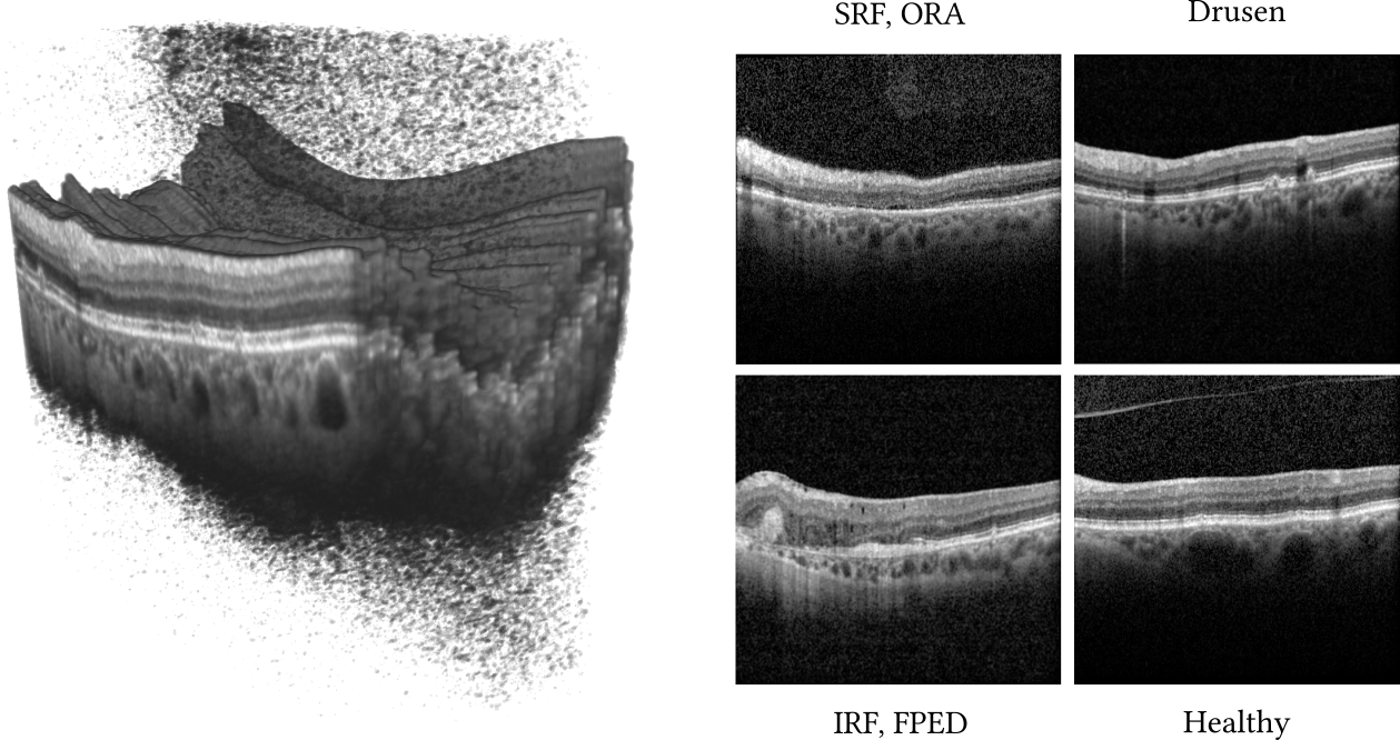
Figure 1: (left) Example of an OCT volume of a patient with AMD. Slices are misaligned, even after post-processing registration. (right) four slices extracted from the volume, each containing a different set of biomarkers indicated for each image.

To support clinicians with OCT-based diagnosis, numerous automated methods have attempted to segment and identify specific biomarkers from OCT scans. For instance, retinal layer [2, 3, 4] and fluid [4] segmentation, as well as drusen detection [5] have previously been proposed. While these methods perform well, they are limited in the number of biomarkers they consider at a time and often use pixel-wise annotations to train supervised machine learning frameworks. Given the enormous annotation task involved in manually segmenting volumes, they are often trained and evaluated on relatively small amounts of data (20 to 100 volumes) [2, 4, 6].

Instead, we present a novel strategy that automatically identifies the presence of a wide range of biomarkers throughout an OCT volume. Our method does not require biomarker segmentation annotations, but rather biomarker tags as to which are present on a given OCT slice. Using a large dataset of OCT slices and annotated tags, our approach then estimates all biomarkers on each slice of a new volume separately. We do this first seperately, without considering adjacent slices, as these are typically highly anisotropic and not aligned within the volume. We then treat these predictions as sufficient statistics for each slice and impose biomarker coherence across slices using a bidirectional Long short-term memory (LSTM) neural network [7]. By doing so, we force our network to learn the wanted biomarker co-dependencies within the volume from slice predictions only, so as to avoid dealing with anisotropic and non-registered slices common in OCT volumes. We show in our experiments that this leads to superior performances over a number of existing methods.

2 Method

We describe here our approach for predicting biomarkers across all slices in an OCT volume. Formally, we wish to predict the presence of $B$ different biomarkers in a volume using a deep network, $f:[0,1]^{S\times{}W\times{}H}\to[0,1]^{S\times{}B}$, that maps from a volume of $S$ slices, $\mathbf{X}\in[0,1]^{S\times{}W\times{}H}$, to a set of predicted probabilities $\hat{\mathbf{Y}}\in[0,1]^{S\times{}B}$. We denote $\hat{\mathbf{Y}}_{sb}$ as the estimated probability that biomarker $b$ occurs in slice $s$.

While there are many possible network architectures for $f$, one simple approach would be to express $f$ as $S$ copies of the same CNN, $f^{\prime}:[0,1]^{W\times{}H}\to[0,1]^{B}$, whereby each slice in the volume is individually predicted. However, such an architecture ignores the fact that biomarkers are deeply correlated across an entire volume. The other extreme would be to define $f$ as a single 3D CNN. Doing so however would be difficult because (1) 3D CNNs assume spatial coherence in their convolutional layers and (2) the output of $f$ would be of dimension $[0,1]^{S\times B}$. While (1) strongly violates OCT volume structure because there are they typically display non-rigid transformations between consecutive OCT slices, (2) would imply training with an enormous amount of training data.

For these reasons, we take an intermediate approach between the above mentioned extremes and express our network as a composition $f=f_{\mathcal{V}}\circ{}f_{\mathcal{S}}$, where $f_{\mathcal{S}}:[0,1]^{S\times{}W\times{}H}\to\mathbb{R}^{S\times{}D}$ processes slices individually and produces a $D$-dimensional descriptor for each slice. Then, $f_{\mathcal{V}}:\mathbb{R}^{S\times{}D}\to[0,1]^{S\times{}B}$ fuses all $S$ slice descriptors and predicts the biomarker probabilities for each slice, whereby taking into account the information of the entire volume. Fig. 2 depicts our framework and we detail each of its components in the subsequent sections.

2.1 Slice network $f_{\mathcal{S}}$

When presented with a volume $\mathbf{X}$, $f_{\mathcal{S}}$ processes each slice independently using the same slice convolutional network, $f^{\prime}_{\mathcal{S}}:[0,1]^{W\times{}H}\to\mathbb{R}^{D}$ that maps from a single slice to a $D$-dimensional descriptor. The output of $f_{\mathcal{S}}$ is then the concatenation of the individual descriptors,

$$f_{\mathcal{S}}(\mathbf{X})=\left[f^{\prime}_{\mathcal{S}}(\mathbf{X}_{1}),\ldots,f^{\prime}_{\mathcal{S}}(\mathbf{X}_{S})\right].$$ (1)

In our experiments, we implemented $f^{\prime}_{\mathcal{S}}$ as the convolutional part of a Dilated Residual Network [8] up to the global pooling layer.

2.2 Volume fusion network $f_{\mathcal{V}}$

Let $\mathbf{D}=f_{\mathcal{S}}(\mathbf{X})\in\mathbb{R}^{S\times{}D}$ be the set of descriptors of a volume $\mathbf{X}$ computed by $f_{\mathcal{S}}$. The fusion network $f_{\mathcal{V}}$ takes $\mathbf{D}$ and produces a final probability prediction $\hat{\mathbf{Y}}$.

The most straightforward architecture for $f_{\mathcal{V}}$ would be a multilayer perception (MLP), which is typical after convolutional layers. However, MLPs make no assumptions about the underlying nature of the data. Consequently, MLPs are hard to train, requiring either huge amounts of training data or resort to aggressive data augmentation techniques, particularly when the dimensionality of the input space is large as in this case. More importantly, a MLP would ignore two important aspects about $\mathbf{D}$: (1) the rows of $\mathbf{D}$ belong to the same feature space that share a common distribution; (2) volumes have spatial structure with respect to the biomarkers within them and slices that are nearby to one another have similar descriptors.

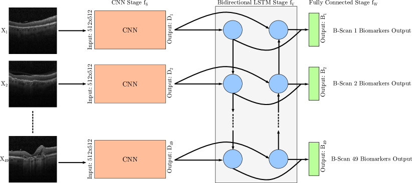
Figure 2: Overview diagram of our apporach including the CNN, $f_{\mathcal{S}}$, the bidirectional LSTM, $f_{\mathcal{V}}$, and the output of the fully connected stage. OCT volumes consist of 49 slices.

To account for this, we use an LSTM to process slices in a sequential way and implicitly leverage spatial dependencies, while performing the same operations on every input (i. e., implicitly assuming a common distribution in the input space). Formally, our LSTM is a network $f_{\ell}:\mathbb{R}^{D}\times{}\mathbb{R}^{H}\to\mathbb{R}^{H}$ that receives a descriptor and the previous $H$-dimensional LSTM state, to produce a new state. We use the LSTM to iteratively process the descriptors $\mathbf{D}$ generating a sequence of LSTM states,

$$\mathbf{h}_{i}=f_{\ell}(\mathbf{D}_{s},\mathbf{h}_{s-1}),\quad s=1,\ldots,S,$$ (2)

where $\mathbf{D}_{s}$ is the descriptor on slice $s$. Additionally, since the underlying distribution of OCT volumes is symmetric, we use the same LSTM to process the descriptors backwards,

$$\mathbf{h}^{\prime}_{i}=f_{\ell}(\mathbf{D}_{s},\mathbf{h}^{\prime}_{s+1}),\quad s=S,\ldots,1,$$ (3)

generating a second sequence of LSTM states. Initial states are $\mathbf{h}_{0}$ and $\mathbf{h}^{\prime}_{S+1}$, respectively.

Note that at each position $s$, $\mathbf{h}_{s}$ and $\mathbf{h}^{\prime}_{s}$ combine the information from the current descriptor $\mathbf{D}_{s}$ with additional information coming from neighboring slices. We then concatenate both states in a single vector and feed it to a final fully connected layer $f_{\omega}:\mathbb{R}^{2H}\to\mathbb{R}^{B}$ that computes the estimated probabilities. The complete volume fusion network $f_{\mathcal{V}}$ is the concatenation of the outputs of $f_{\omega}$ for all the slices:

$$f_{\mathcal{V}}(\mathbf{D})=\left[f_{\omega}([\mathbf{h}_{1},\mathbf{h}^{\prime}_{1}]),\ldots,f_{\omega}([\mathbf{h}_{S},\mathbf{h}^{\prime}_{S}])\right].$$ (4)

2.3 Training

Training $f$ requires a dataset of $M$ annotated volumes, $\mathcal{D}=\{(\mathbf{X}^{(m)},\mathbf{Y}^{(m)})\}_{m=1}^{M}$ where for each volume $\mathbf{X}^{(m)}$ a set of binary labels $\mathbf{Y}^{(m)}$ is provided. $\mathbf{Y}^{(m)}_{sb}$ is 1 if biomarker $b$ is present in slice $\mathbf{X}^{(m)}_{s}$. We then use the standard binary cross entropy as our loss function,

$$\ell(\mathbf{Y},\hat{\mathbf{Y}})=-\sum_{s}\sum_{b}(1-\mathbf{Y}_{sb})\log(1-\hat{\mathbf{Y}}_{sb})+\mathbf{Y}_{sb}\log\hat{\mathbf{Y}}_{sb},$$ (5)

where $\hat{\mathbf{Y}}=f(\mathbf{X})$ is the estimation of our network for a given volume. The goal during training is then to minimize the expected value of the loss $\ell$ over the training dataset $\mathcal{D}$.

While we could perform this minimization with a gradient-based method in an end-to-end fashion from scratch, we found that a two-stage training procedure helped boost performances at test time. In the first stage, we train the slice network $f^{\prime}_{\mathcal{S}}$ alone to predict the biomarkers of individual slices. More specifically, we append a temporary fully connected layer $f_{t}:\mathbb{R}^{D}\to[0,1]^{B}$ at the end of $f^{\prime}_{\mathcal{S}}$, and then minimize a cross entropy loss while presenting to the network randomly sampled slices from $\mathcal{D}$. In the second stage, we fix the weights of $f^{\prime}_{\mathcal{S}}$ and minimize the loss of Eq. (5) for the whole architecture $f$ updating only the weights of the volume fusion network $f_{\mathcal{V}}$.

3 Experiments

3.1 Data

Our dataset consists of 416 volumes (originating from 327 individuals with Age-Related Macula Degeneration and Diabetic Retinopathy) whereby each volume scan consists of $S=49$ slices for a total of 20’384 slices. Volumes were obtained using the Heidelberg Spectralis OCT and each OCT slice has a resolution of $496\times 512$ pixels. Trained annotators provided slice level annotations for 11 common biomarkers: Subretinal Fluid (SRF), Interetinal Fluid (IRF), Hyperreflective Foci (HF), Drusen, Reticular Pseudodrusen (RPD), Epiretinal Membrane (ERM), Geographyic Atrophy (GA), Outer Retinal Atrophy (ORA), Intraretinal Cysts (IRC), Fibrovascular PED (FPED) and Healthy. The dataset was randomly split $90\%/10\%$ for training and testing purposes, making sure that no volume from the same individual was present in both the training and test sets. These sets contained a total of 18’179 and 2’205 slices, respectively. The distribution of biomarkers in the training and test sets are reported in Table 1. For all our experiments, we performed 10-fold cross validation, where the training set was split into a training (90%) and validation (10%) set.

3.2 Parameters and baselines

For our approach, we set $D=512$ for the size of the $f_{\mathcal{S}}$ descriptors and $H=512$ for the size of the LSTM hidden state. We train the fusion stage using a batch size of 4 volumes, while training using SGD with momentum of $0.9$ and a base learning rate of $10^{-2}$ which we decrease after 10 epochs of no improvement in the validation score.

To demonstrate the performance of our approach, we compare it to the following baselines:

• Base: the output of $f_{\mathcal{S}}$ (e.g. no slice fusion).

• MLP: output of size $49\times 11$ using the $49\times 512$ sized feature matrix from the Base classifier.

• Conv-BLSTM: fuses the last convolutional channels of $f_{\mathcal{S}}$ with a size of $(49,64,64,256)$ and a hidden state of $H=256$ channels. This is then followed by a global pooling and a fully connected layer.

• Conditional Random Field (CRF): trained to learn co-occurrence of biomarkers within each slice and to smooth the predictions for each biomarker along different slices of the volume. Logit outputs of the Base classifier are used as unary terms, and learned pairwise weights are constrained to be positive to enforce submodularity of the CRF energy. We use the method from [9] for training and standard graph-cuts for inference at test time.

For all methods we use the same Base classifier and train it as a multi-label classification task using a learning rate of $10^{-2}$, a batch size of 32 with SGD and a momentum of $0.9$. Rotational and flipping data augmentation was applied during training. We retain the best model for evaluation and do not perform test time augmentation or cropping. The network was pre-trained on ImageNet [10].

Our primary evaluation metric are the micro and macro mean Average Precision (mAP). In addition, we also report the Exact Match Ratio (EMR) which is equal to the percentage of slices predicted without failing to detect any biomarker in it. The mAP of the CRF baseline is not directly comparable as the CRF output is binary, hence allowing only a single preciscion-recall point to be evaluated. We therefore also state the maximum F1 scores for each method.

3.3 Results

Table 1 reports the performances of all methods. Using the proposed method we see an increase in mAP across all biomarkers except for GA and ORA. Both biomarkers have a very low sample size in the test set. The proposed method outperforms all other fusion methods in terms of mAP and F1 score and considerably improves over the unfused baseline, which confirms our hypothesis that inter-slice dependencies can be used to increase the per slice performance. The poor performance of the Convolutional BLSTM can be explained due to the misalignment of adjacent slices.

In Fig. 3, we show a typical example illustrating the performance improving ability of our proposed method. In particular, we show here the prediction of our approach on each slice for each biomarker and highlight three consecutive slices of the tested volume (right). For comparison, we also show the corresponding ground-truth (top left) and the outcome from the Base classifier (middle left). Here we see that our approach is capable of inferring more accurately the set of biomarkers across the different slices.

Biomarker	Base	MLP	Conv-BLSTM	CRF	Proposed
Healthy (5310/494)	0.797$\pm$0.023	0.730$\pm$0.025	0.795$\pm$0.013	-	0.800$\pm$0.022
SRF (942/103)	0.847$\pm$0.024	0.796$\pm$0.043	0.877$\pm$0.030	-	0.905$\pm$0.017
IRF (2019/339)	0.691$\pm$0.044	0.705$\pm$0.039	0.701$\pm$0.052	-	0.761$\pm$0.047
HF (4261/684)	0.877$\pm$0.008	0.839$\pm$0.010	0.863$\pm$0.018	-	0.896$\pm$0.007
Drusen (3990/399)	0.762 $\pm$0.024	0.731$\pm$0.024	0.766$\pm$0.029	-	0.775$\pm$0.038
RPD (1620/146)	0.291$\pm$0.044	0.302$\pm$0.036	0.288$\pm$0.069	-	0.335$\pm$0.077
ERM (4338/670)	0.885$\pm$0.009	0.849$\pm$0.014	0.850$\pm$0.022	-	0.903$\pm$0.010
GA (897/67)	0.557$\pm$0.063	0.234$\pm$0.047	0.330$\pm$0.049	-	0.556$\pm$0.057
ORA (1999/84)	0.151$\pm$0.018	0.105$\pm$0.008	0.143$\pm$0.025	-	0.131$\pm$0.019
IRC (3097/553)	0.932$\pm$0.006	0.880$\pm$0.011	0.928$\pm$0.012	-	0.940 $\pm$0.006
FPED (3654/387)	0.931$\pm$0.007	0.920 $\pm$0.008	0.936$\pm$0.009	-	0.949$\pm$0.006
mAP (micro)	0.814$\pm$0.006	0.768$\pm$0.012	0.794$\pm$0.010	0.599$\pm$0.003	0.834$\pm$0.012
mAP (macro)	0.702$\pm$0.008	0.645$\pm$0.009	0.680$\pm$0.012	0.523$\pm$0.006	0.723$\pm$0.014
EMR*	0.423$\pm$0.015	0.164$\pm$0.048	0.413$\pm$0.019	0.440$\pm$0.003	0.438$\pm$0.011
F1*	0.676$\pm$0.006	0.502$\pm$0.024	0.676$\pm$0.011	0.649$\pm$0.013	0.694$\pm$0.009

Table 1: Experimental results comparing our proposed method to other approaches. The per-biomaker scores are shown as mean Average Precision (mAP). The training and test label occurrence is stated beside the biomarker name (training/test). (*) threshold taken at the max F1 score.

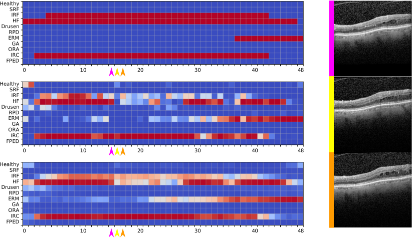
Figure 3: Volume classification example, where (top left) depicts the ground truth, (middle left) the Base classification and (bottom left) our proposed method. Warm colors indicate higher likelihood of presence. (Right) Three consecutives slices where the Base classifier incorrectly misses biomarker IRF in the center slice (yellow). Our proposed method manages to fuse information from adjacent slices (pink and orange) to infer the proper prediction.

4 Conclusion

We have presented a novel method to identify pathological biomarkers in OCT slices. Our approach involves detecting biomarkers first slice by slice in the OCT volume and then using a bidirectional LSTM to coherently adjust predictions. As far as we are aware, we are the first to demonstrate that such fine-grained biomarker detection can be achieved in the context of retinal diseases. We have shown that our approach performs well on a substantial patient dataset outperforming other common fusion methods. Future efforts will be focused on extending these results to infer pixel-wise segmentations of found biomarkers relying solely on the per-image labels.

References

- [1] Bourne, R., et al.: Magnitude, temporal trends, and projections of the global prevalence of blindness and distance and near vision impairment: a systematic review and meta-analysis. Lancet Global Health 5 (2017) e888 – e897
- [2] Apostolopoulos, S., De Zanet, S., Ciller, C., Wolf, S., Sznitman, R.: Pathological OCT Retinal Layer Segmentation Using Branch Residual U-Shape Networks. In: Medical Image Computing and Computer-Assisted Intervention. (2017) 294–301
- [3] Hussain, M.A., Bhuiyan, A., Turpin, A., Luu, C.D., Smith, R.T., Guymer, R.H., Kotagiri, R.: Automatic Identification of Pathology-Distorted Retinal Layer Boundaries Using SD-OCT Imaging. IEEE Transactions on Biomedical Engineering 64(7) (2017) 1638–1649
- [4] Roy, A.G., Conjeti, S., Karri, S.P.K., Sheet, D., Katouzian, A., Wachinger, C., Navab, N.: ReLayNet: retinal layer and fluid segmentation of macular optical coherence tomography using fully convolutional networks. Biomedical Optics Express 8(8) (2017)
- [5] Zhao, R., Camino, A., Wang, J., Hagag, A.M., Lu, Y., Bailey, S.T., Flaxel, C.J., Hwang, T.S., Huang, D., Li, D., Jia, Y.: Automated drusen detection in dry age-related macular degeneration by multiple-depth,en faceoptical coherence tomography. Biomedical optics express 8(11) (2017) 5049–5064
- [6] Bogunovic, H., et al.: RETOUCH -the retinal OCT fluid detection and segmentation benchmark and challenge. IEEE Trans. Med. Imaging (February 2019)
- [7] Graves, A., Fernández, S., Schmidhuber, J.: Bidirectional lstm networks for improved phoneme classification and recognition. In: Artificial Neural Networks: Formal Models and Their Applications. (2005) 799–804
- [8] Yu, F., Koltun, V., Funkhouser, T.: Dilated residual networks. (May 2017)
- [9] Szummer, M., Kohli, P., Hoiem, D.: Learning crfs using graph cuts. Volume 5303. (10 2008) 582–595
- [10] Russakovsky, O., Deng, J., Su, H., Krause, J., Satheesh, S., Ma, S., Huang, Z., Karpathy, A., Khosla, A., Bernstein, M., Berg, A.C., Fei-Fei, L.: ImageNet Large Scale Visual Recognition Challenge. International Journal of Computer Vision 115(3) (2015) 211–252