A Subjective Interestingness measure for Business Intelligence explorations

Abstract

This paper addresses the problem of defining a subjective interestingness measure for BI exploration. Such a measure involves prior modeling of the belief of the user. The complexity of this problem lies in the impossibility to ask the user about the degree of belief in each element composing their knowledge prior to the writing of a query. To this aim, we propose to automatically infer this user belief based on the user’s past interactions over a data cube, the cube schema and other users’ past activities. We express the belief under the form of a probability distribution over all the query parts potentially accessible to the user, and use a random walk to learn this distribution. This belief is then used to define a first Subjective Interestingness measure over multidimensional queries. Experiments conducted on simulated and real explorations show how this new subjective interestingness measure relates to prototypical and real user behaviors, and that query parts offer a reasonable proxy to infer user belief.

1 Introduction

Business intelligence (BI) exploration can be seen as an iterative process that involves expressing and executing queries over multidimensional data (or cubes) and analyzing their results, to ask more focused queries to reach a state of knowledge that allows to answer a business question at hand. This complex task can become tedious, and for this reason, several approaches have been proposed to facilitate the exploration by pre-fetching data [27], detecting interesting navigation paths [29], recommending appropriate queries based on past interactions [2] or by modeling user intents [14].

Ideally, such systems should be able to measure to which extent a query would be interesting for a given user prior to any exploration. Indeed, as illustrated in [7] and first elicited in [30] in the context of Explorative Data Mining (EDM), the interestingness of a pattern depends on the problem at hand, and, most importantly, on the user that extracts the pattern. An interestingness measure for such explorative tasks should therefore be tailored for a specific user.

Following the idea of subjective interestingness measures initiated and developed by De Bie [5], our aim is to measure the subjective interestingness of a query a expressed by a coherent set of query parts, based on the prior knowledge that the user has about the cube and the cost for the user to understand the query and its evaluation.

It is therefore crucial, before reaching the definition of such an interestingness measure for BI, to be able to transcribe, with an appropriate information-theoretic formalism, the prior user knowledge, also called belief, on the data. De Bie proposes to represent this belief as a probability distribution over the set of data. However, it is clearly not possible to explicitly ask a user about the degree of belief in each element composing their knowledge prior to each query, let alone identifying on which element of knowledge expressing this probability distribution. This motivates the investigation of approaches for automatically estimating the user’s belief based on their implicit feedback. Let us now consider the following example to illustrate the difficulty of estimating probabilities for the belief.

Figure 1: Toy SSB benchmark session

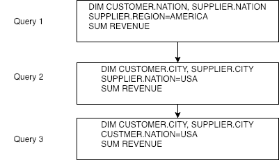
Example

Consider the exploration over the schema of the Star Schema Benchmark [24], consisting of $3$ queries, as illustrated in Figure 1, and loosely inspired by session 3 of the SSB’s workload. For the sake of readability, only the relevant query parts (grouping set, filters and measures) are shown. This example showcases the short session initiated by a user that explores the cube looking for information on revenue some company makes in different locations. Assume we are interested in recommending a query to the user for continuing the exploration. This recommendation should be both connected to the most used query parts, so as not to loose focus, but also should bring new, possibly unexpected information, so as not to feed the user with already known or obvious information. A naive solution would be to use the set of all possible query parts as the set of data and to express the belief based on the frequency of each query part in the past user history. From the session in Figure 1 it is possible to compute the number of occurrences of each query part (for instance, SUM REVENUE appears 3 times, CUSTOMER.CITY 2 times, while SUPPLIER.REGION=AMERICA appears only once, etc.). However, this simple representation raises major problems: first, the vector of user belief computed from the number of occurrences will mostly contain zero values because the majority of users will concentrate their exploration to a certain region of the data cube. Second, this belief would not give any probability to query parts such as CUSTOMER.NATION=CANADA, while if user knows about AMERICA and USA, she is likely to have a basic knowledge about sibling countries to USA in the dimension CUSTOMER.NATION. Finally, it may also be taken advantage of other users’ former explorations, as a proxy of what the current user might find interesting.

This example stresses the need for an approach to define the belief based on the users’ past activity, as well as an information about how knowledge is structured, which, in the case of the data cube, can be found in the cube schema. We note that while previous works already investigated surprising data in cubes (see e.g., [29, 10]), to the best of our knowledge none of them did so by explicitly modeling a user’s belief.

As a first step in this direction, our previous paper [11] tracks user belief in BI interactions for measuring the subjective interestingness of a set of queries executed on a data cube. This approach builds a model of the user’s past explorations that is then used to infer the belief of the user about the query parts being useful for the exploration. Contrary to the context of pattern mining [5] where in general no metadata information is available, the query parts that are employed in this model cannot be considered agnostically of the cube schema, that the user typically knows. In this context, the method introduced in [11] takes advantage of the schema to infer what a user may or may not know based on what has been already visited and what is accessible from the previous queries. The belief of a user is defined as a probability distribution over the set of query parts coming from the log of past activities and the cube schema. This probability distribution is learned as the resulting stationary distribution of a modified topic-specific PageRank algorithm, where the underlying graph topology matrix is based on previous usage and the schema of the cube, and where a teleportation matrix that corresponds to a specific user model is introduced to ensure connectivity. Finally, [11] takes advantage of the artificial exploration generator CubeLoad [26] that mimics several prototypical user behaviors to evaluate qualitatively and quantitatively divergences in the estimated user belief.

The work presented here improves on that introduced in [11] with several major contributions, both at the methodological level and at the experimental level:

• it refines the belief model by taking into account the filter values of the query parts. This is a strong bottleneck since it adds a lot of vertices in the graph used to compute user belief. To solve this problem, new rules to build the graph are introduced in Section 4.2 ;

• as stated before, this new belief model benefits from information from the cube schema, the past logs and an actual user profile represented by her explorations. All the underlying operations are now defined as simple graph manipulation primitives and allow for an easier understanding of the whole process ; reproducibility of the experiments is permitted thanks to the shared code repository ;

• according to these new construction rules, the approach now results in only one strongly connected graph which avoids the need for a teleportation matrix and ensures a cleaner convergence mechanism. Details of the simplified PageRank algorithm is provided in Section 3.3 ;

• as in [11], we introduce a real valued parameter $\alpha\in[0,1]$ that allows to give more or less importance to the user specific exploration bias in the computation of the belief distribution. This parameter is at the core of our experiments as it allows to reveal, when set close to $1$, significant differences in belief and subjective interestingness models ;

• our approach now contains a simple yet efficient incremental mechanism that allows to track the evolution of the belief during an exploration as described in Section 4.3 ;

• finally, this paper introduces a first formalization of a subjective interestingness measure for Business Intelligence explorations based on the belief distribution and on a simple measure of the complexity of a query formed by several query parts, as described in Section 5.

As in [11], one difficulty stands in the evaluation of our proposal, as there is no ground truth available. In this context, we propose several experiments:

• an updated qualitative and a quantitative evaluation of the belief distributions for several simulated user profiles using CubeLoad generator [26] and new experiments on real data with the DOPAN workload [12] ;

• a set of novel experiments that a posteriori estimates the subjective interestingness of queries in simulated and real explorations from CubeLoad and the DOPAN workload.

Experimental conclusions show that our approach to model user belief and subjective interestingness from a graph of query parts: ($1$) behaves as expected on both prototypical user behaviors and real user explorations, and ($2$) indicates that query parts are a good proxy to infer user belief.

This paper is organized as follows: Section 2 motivates the use of user belief and subjective interestingness measure in the context of BI exploration. Section 3 introduces the concepts used in our approach: formal definitions BI explorations, query parts and concepts related to Subjective Interestingness and PageRank algorithm. Section 4 introduces the graph based user belief model using past explorations and schema as inputs, and introduces a novel algorithm to deal with incremental belief estimation. Section 5 introduces the Subjective Interestingness definition based on said model. Finally, Sections 6 and 7 present our experiments to assess our belief model and our Subjective Interestingness measure, both on artificially generated explorations and on real user explorations. Finally, Section 8 discusses related work and Section 9 concludes and draws perspectives.

2 Our vision of User Centric Data Exploration

This section describes how the knowledge of a user belief, and by extension a subjective interestingness measure, could be used to improve the user’s experience in the context of interactive data exploration. This example highlights the main scientific challenges of such task, some of them being left as future work as the present paper exclusively focuses on a first expression of user belief and a derived subjective interestingness measure in the context of data cube exploration.

Figure 2: Envisioned use of belief and subjective interestingness measures in data exploration

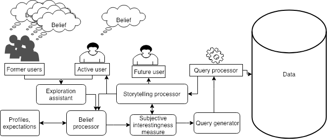
In our vision, illustrated in Figure 2, human remains in the loop of data exploration, i.e., the exploration is not done fully automatically, but we aim at making it less tedious. All users, naive or expert, willing to explore a dataset, express their information need through an exploration assistant. This assistant is left with the task of deriving from the user’s need the actual queries to evaluate over the data source. This exploration assistant communicates with a belief processor that is responsible for the maintenance of the user’s profile, i.e., a model of that user, in the sense that it includes an estimation of the actual belief unexpressed by the user. This belief is manifold and concerns e.g., hypotheses on the value of the data, the filters to use, how the answer should be presented, etc. The belief processor activates a series of subjective interestingness measures that drives the query generator for deriving and recommending the most interesting queries for this user, in the sense that they produce relevant, unexpected, diverse answers, avoiding undesirable artifacts such as biased or false discoveries, the so-called cognitive bubble trap, etc. These answers and recommendations are packaged (e.g., re-ranked, graphically represented) by the storytelling processor before being displayed to the user and sent to the belief processor for profile updating.

Notably, thanks to the belief processor, once enough diverse users are modeled, the storytelling processor may cope with the cold start problem of generating recommendation for unknown users (the future user of Figure 2), e.g., by removing bias introduced by common beliefs.

The work presented in this paper is the first step in the implementation of this vision. We first concentrate on cube exploration, expressing the belief over query parts and deriving an incremental Subjective Interestingness measure on queries. Noticeably, all our definitions take advantage of the peculiarities of the data cube exploration context to be on par with what a human analyst would consider interesting.

3 Preliminaries

This section introduces the basic definitions of our framework.

3.1 BI explorations

Our work considers BI explorations, i.e., sequences of OLAP queries over a database instance under a star schema, called datacube.

Let $D$ be a database schema, $I$ an instance of $D$ and $Q$ the set of formal queries one can express over $D$. For simplicity, in this paper, we consider relational databases under star schemata, queried with multidimensional queries. Let $A$ be the set of attributes of the relations of $D$. Let $M\subset A$ be a set of attributes defined on numerical domains called measures. Let $H=\{h_{1},\ldots,h_{n}\}$ be a finite set of hierarchies, each characterized by (1) a subset $Lev(h_{i})$ of attributes called levels and (2) a roll-up total order $\succeq_{h_{i}}$ of $Lev(h_{i})$. We denote by $adom(A)$ the set of all constants appearing the instance $I$ of $D$ for attribute $A$. For each hierarchy $h_{i}$, $Lev(h_{i})$ includes a top-most level $l_{i}^{ALL}$ such that $\nexists l\in Lev(h_{i}),l_{i}^{ALL}\succeq_{h_{i}}l$. This level only has one value called $all_{i}$, i.e., $adom(l_{i}^{ALL})=\{all_{i}\}$. For any two consecutive levels $l^{1}_{i},l^{2}_{i}$ of a hierarchy $h_{i}$, function $children(m)$ applied to $m\in adom(l^{1}_{i})$ returns the set of values in $adom(l^{2}_{i})$ that are direct children of $m$ according to $h_{i}$.

To simplify, we describe an OLAP query $q$ in $Q$ as a set of query parts. Note that the term query parts can undergo different meanings. Coherent with our objective of taking into account both usage (i.e., previous explorations) and cube schema, our query part definitions encompasses both. We rely on the definition of query part provided by [26], where the authors consider it is one constituent of a

multidimensional query consisting of (i) a group-by (i.e., a set of hierarchy levels on which measure values are grouped); (ii) one or more measures whose values are returned (the aggregation operator used for each measure is defined by the multidimensional schema); and (iii) zero or more selection predicates, each operating on a hierarchy level.

However, in our case, a query part is not necessarily attached to a query already expressed by some user, since we aim at considering also query parts that might be used in the future.

Formally, a query part is either (i) a level $l$ of a hierarchy in $H$, (ii) a measure in $M$, or the member $v$ of a simple Boolean predicate of the form $l=v$, where $l$ is a level of a hierarchy in $H$, and $v$ is a constant in $adom(l)$. Note that each member $v$ identifies its level and hierarchy. Given a database $D$ we call $P_{D}$ the set of query parts. In what follows, queries are confounded with their sets of query parts, unless otherwise stated, and we assume a function $parts(q)$ that applied over a query $q$ returns the subset of $P_{D}$ containing its query parts.

Finally, a BI exploration $s$ is a sequence $[q_{1},\ldots,q_{p}]$ of $p$ OLAP queries, and a log is a set of explorations.

3.2 Interestingness for exploratory data mining

The framework proposed by De Bie [5], in the context of exploratory data mining, is based on the idea that the goal of any exploratory data mining task is to pick patterns that will result in the best updates of the user’s knowledge or belief state, while presenting a minimal strain on the user’s resources. In De Bie’s proposal, the belief is defined for each possible value for the data from the data space and can be approximated by a background distribution.

As a consequence, a general definition for this interestingness measure (IM) is a real-valued function of a background distribution, that represents the belief of a user, and a pattern, that is to say the artifact to be presented to the explorer. Given a set $\Omega$, the data space, and a pattern $\Omega^{\prime}$ a subset of $\Omega$, the belief is the probability P$(\Omega^{\prime})$ of the event $x\in\Omega^{\prime}$, i.e., the degree of belief the user attaches to a pattern characterized by $\Omega^{\prime}$ being present in the data $x$. In other words, if this probability is small, then the pattern is subjectively surprising for the explorer and thus interesting. In this sense, the IM is subjective in that it depends on the belief of the explorer. De Bie also proposes to weight this surprise by the complexity of the pattern $\Omega^{\prime}$ as follows:

$$IM_{DeBie}(P,\Omega^{\prime})=\frac{-log(P(\Omega^{\prime}))}{descComp(\Omega^{\prime})}$$ (1)

where $P$ represents the user belief, i.e., the background distribution of the pattern $\Omega^{\prime}$ over the set of data $x$ and $descComp(\Omega^{\prime})$ denotes the description complexity of a pattern $\Omega^{\prime}$.

The data mining process consists in extracting patterns and presenting first those that are subjectively interesting, and then refining the belief background distribution based the newly observed pattern $\Omega^{\prime}$. The key to such modeling as proposed by De Bie lies in the definition of the belief of each user for all possible patterns and how it should evolve based on new patterns explored during time.

3.3 PageRank

Initially, the PageRank algorithm is designed to estimate the relative importance of web pages as a probability to end up on this web page after an infinite surf on the web [9]. This algorithm is based on ergodic Markov Chains. A Markov Chain models a collection of states and transitions probabilities from a state to the next. At a particular time t, a random walker is assumed to be in a unique state of the chain. We are interested by the probability distribution over the states after some time. After an infinite amount of time, this distribution is called the stationary distribution, if it exists. As the transitions probabilities themselves cannot change with time, these chains can be represented as simple directed graphs with the different possible states as nodes and the transitions as edges with their assigned probabilities. A Markov Chain can also be represented as an (N,N) matrix, where N is the number of possible states. A Markov Chain that is aperiodic and where all states are connected with all other states by a sequence of states whose transitional probabilities are not zero has the ergodic property. In other words, it is possible to reach any state from any initial state with enough time. This implies that a stationary distribution over the possible states exists and is unique after an infinite number of iterations, independently of the starting state.

In the classical Page Rank algorithm used for the web, the pages are the possible states of the Markov Chain and the hyperlinks are the transitions between states. The transitional probabilities from a particular page are proportional to the number of hyperlinks targeting a common page. Thus, to rank the pages by popularity, one needs to find the stationary distribution over the pages. These are the probabilities of landing on a page after surfing for a long time, starting from any page. The stationary distribution, called the PageRank vector $PR$, is the solution to the following equation:

$$PR=M\times PR$$ (2)

where $M$ is the stochastic transition matrix of the graph of web pages hyperlinks.

Our approach considers query parts as states in a Markov chain and Section 4.2 explains how transitional probabilities are defined.

4 Inferring user belief from schema and log usage

This section presents our first contribution and addresses the following questions: ($1$) what is user belief in BI exploration? ($2$) How to estimate it? ($3$) How to make it evolve during an exploration?

4.1 What is user belief in BI?

Ideally, in the context of BI exploration, the user belief would be a probability the user attaches to the statement ”I believe the value of this cell is exactly this one”. Modeling such a belief is one of our long term perspectives, as such this would raise several questions such as: ($1$) how to ensure efficiency while executing all the queries to update the belief over cells? ($2$) How to cope with the combinatorial complexity of expressing the belief over subsets of cells rather than a single cell? ($3$) How to update the belief distribution over cells when observing aggregated values at higher level of granularity? As an example, Sarawagi in her seminal work [28] to estimate user belief, restricts her study to the sum measure paired with an assumption of uniform distribution to locally estimate belief on cells when exploring aggregates. Sarawagi’s work relies on the following assumptions: belief is only expressed over a limited set of cells (relating to those already explored) and the cube instance and past query answers are available to estimate this belief.

In a first methodological step towards this ambitious direction, we use query parts as proxies to estimate this user belief. We consider in this work that the user belief is the importance the user attaches to the statement ”I believe this query part is relevant for my exploration”. In some sense, we consider query parts as pieces of knowledge about the data that reduce the set of possible values it may take from the original data space, inspired by the De Bie’s view of explorative pattern mining [4, 20] and as illustrated in Figure 3.

Figure 3: Aligned with De Bie’s framework, query parts can be seen as restrictions to the original data space in the case of an OLAP cube exploration

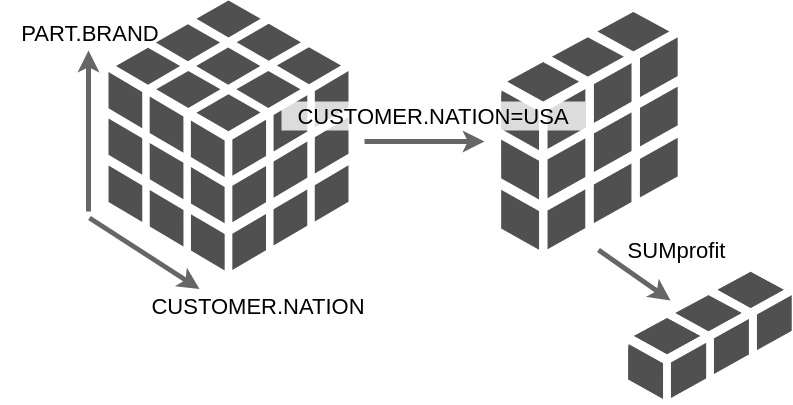
We propose to define the user belief over the set of query parts for the following reasons. First, the set of query parts is measurable (and usually reasonable in size) and thus respects the formal constraints in the model of De Bie [5] to extend the belief to an interestingness measure. Second, database instance or query answers may not be available, e.g., for privacy or confidentiality reasons, when query logs are anonymized. Finally, query parts provide a finer level to work with compared to queries. Working at the query level would end-up with a very sparse representation of the data space, as the probability that two queries occur in the same exploration is much lower than the probability that two query parts appear in the same query or exploration. Moreover, when considering query parts, the most interesting ones for the user may appear in several consecutive queries and thus might have more prominent probability values.

As we cannot ”brain-dump” the user, the belief is approximated by the importance of the available query parts. The challenge lies in a way to find this probability distribution over a possibly infinite or too large set of query parts even if we restrict to the attributes in a given schema. Practically, in order to avoid to deal with all these query parts, we restrict to those appearing in a query log or in the schema, where only the active domain of the attributes is considered. Subjectiveness is ensured by the importance attached to the query parts appearing of the user’s log of former explorations.

4.2 Using PageRank as a belief function

Once restricted the set of query parts, we still need to compute their relative importance expressed as a probability distribution for a specific user. As explained previously, this is done by a PageRank (PR) algorithm that computes the probability for a user $u$ to end up on a query part $p$ when using the cube schema during the exploration, knowing past explorations by other users and knowing the profile of $u$. A naive assumption that could be made on this set of parts for an initial background distribution is that all parts not seen by the user are equally probable and those seen are as probable as often they appear in the user’s log. This would ignore many behaviors evidenced in the user explorations and connections of parts in the schema of the cube. Our approach incorporates those elements.

Given a database schema $D$ with query parts $P_{D}$, the input to the PageRank algorithm is a directed graph of query parts $G=\langle P_{D},E\rangle$, computed by Algorithms 1, 2 and 4 respectively, as detailed in the following paragraphs.

Note that compared to our preliminary work [11], we use a more elaborated technique for building the graph. In particular, we now consider as vertices the filter values (i.e., members) of potential selection predicates instead of the hierarchy levels on which they apply. This brings richer information about the data in our approach without changing the overall method described in [11]. The relationships between the selection predicates and their associated levels in the hierarchy are conserved but transcribed into the edges (see below and in Algorithm 2).

Algorithm 1 Schema based graph construction

1:function BuildSchemaGraph($D$)

2:Require:A schema $D$

3:Ensure:A graph of query parts

4:     $V\leftarrow P_{D}$, $E\leftarrow\emptyset$

5:     for $h_{i}\in H$ do $\triangleright$ For each hierarchy in the schema

6:         $E\leftarrow LinkMember(E,\{all_{i}\})$ $\triangleright$ Connects members

7:         for $m\in adom(l)$ such that $l\in Lev(h_{i})$ do

8:              $E\leftarrow E\cup\{\langle m,l,1\rangle,\langle l,m,1\rangle\}$          

9:         for $l^{1}_{i},l^{2}_{i}\in Lev(h_{i})$ such that $l^{1}_{i}\succeq_{i}l^{2}_{i}$ and $\nexists l^{3}_{i},l^{1}_{i}\succeq_{i}l^{3}_{i}\succeq_{i}l^{2}_{i}$ do

10:              $E\leftarrow E\cup\{\langle l^{1}_{i},l^{2}_{i},1\rangle,\langle l^{2}_{i},l^{1}_{i},1\rangle\}$               

11:     return $\langle V,E\rangle$

12:function LinkMember(E, m) $\triangleright$ Recursively scans the hierarchy tree

13:     $C\leftarrow children(m)$

14:     if $C=\emptyset$ then return E      

15:     for $c\in C$ do

16:         $E\leftarrow E\cup\{\langle m,c,1\rangle,\langle c,m,1\rangle\}$

17:         $E\leftarrow LinkMember(E,c)$      return E

Algorithm 2 Log based Graph construction

1:function BuildLogGraph($L,G$)

2:Require:A log $L$ and a graph $G=\langle V,E\rangle$

3:Ensure:A graph of query parts

4:     for $s=[q_{1},\ldots,q_{p}]\in L$ do

5:         for $i\in\llbracket 1,p-1\rrbracket$ do

6:              $P_{i}\leftarrow parts(q_{i})$, $P_{i+1}\leftarrow parts(q_{i+1})$

7:              $V\leftarrow V\cup P_{i}\cup P_{i+1}$

8:              for $p_{1}\in P_{i}$ do

9:                  for $p_{2}\in P_{i}$ do

10:                       if $\langle p_{1},p_{2},v\rangle$ in $E$ then

11:                           $E\leftarrow(E\setminus\{\langle p_{1},p_{2},v\rangle\})\cup\{\langle p_{1},p_{2},v+1\rangle\}$

12:                       else

13:                           $E\leftarrow E\cup\{\langle p_{1},p_{2},1\rangle\}$                                          

14:                  for $p_{next}\in P_{i+1}$ do

15:                       if $\langle p_{1},p_{next},v\rangle$ in $E$ then

16:                           $E\leftarrow(E\setminus\{\langle p_{1},p_{next},v\rangle\})\cup\{\langle p_{1},p_{next},v+1\rangle\}$

17:                       else

18:                           $E\leftarrow E\cup\{\langle p_{1},p_{next},1\rangle\}$                                                                      

19:     return $\langle V,E\rangle$

Schema based construction rules

To represent the global topology induced by a database schema $D$, a graph is constructed as follows,: (i) there is an edge between any two consecutive levels of a hierarchy ; (ii) for any there is an edge between a member and its direct children in the hierarchy of this member ; (iii) finally, there is an edge between each member and its level attribute. Details about the implementation of these rules are provided in Algorithm 1.

Log usage construction rules

To represent the activity of a user or group of users, a graph can be constructed as follows. There is an edge $e$ from query part $p_{1}$ to query part $p_{2}$ and an edge $e^{\prime}$ from $p_{2}$ to $p_{1}$ if $p_{1}$ and $p_{2}$ appear together in the same query. There is also an edge $e$ from query part $p_{1}$ to query part $p_{2}$ if $p_{1}$ is in a query that precedes, in an exploration, another query where $p_{2}$ appears. As described in Algorithm 2, those rules can be applied either to generate the graph of all users past queries or to produce the graphs of a specific user by restricting the log used as input. Note that Algorithm 2 can either be used to update a pre-existing schema graph or, if the input graph is set to an empty graph, only build a new graph related to usage.

Introducing subjectivity

Algorithms 1 and 2 can be used to construct a graph that represents a general topology of the query space (Algorithm 1) and transcribes important relationships established by the past users explorations (Algorithm 2, called with a query log detailing the past activities of all users). This graph $G_{t}$, called the topology graph from now on, is however not subjective in any way. It has to be biased toward a specific user $U$, represented by the subset of the query parts occurring in their sessions. To this end, Algorithm 2 can be called over the query log of user $U$, and defines $G_{u}=\langle P_{D},E_{u}\rangle$ called the specific subjective user centered graph.

Constructing the PageRank graph

Once we have a graph representing the topology induced by the schema and the past logs graph, $G_{t}$, and a specific subjective user centered graph, $G_{u}$, we can aggregate them to produce the graph that will serve as an input for the PageRank algorithm described in Section 3.3. To that aim, Algorithm 3 introduces a real parameter $\alpha\in[0,1]$ that allows to give more or less weight to graph $G_{u}$ compared to the topology graph $G_{t}$. Indeed, the topology graph is generally very large and the subjective user centered graph only modifies a small portion of it which may be barely noticeable in terms of belief distribution. In that sense, $\alpha$ can be seen as a normalization factor, as it can be used to control the relative importance of the user’s log against the general log and topology inherited from the schema.

Algorithm 3 Graphs merging algorithm

function Merge($G_{1},G_{2},\alpha$)

Input: 2 graphs $G_{1}=\langle V_{1},E_{1}\rangle$ and $G_{2}=\langle V_{2},E_{2}\rangle$ and a real value $\alpha\in[0,1]$

Output: a merged graph $G=\langle V,E\rangle$

     $V\leftarrow V_{1}\cup V_{2}$ $\triangleright$ Initialize the set of vertices of new graph

     for $\langle p_{1},p_{2},v\rangle\in E_{1}$ do $\triangleright$ Add all updated edges from $G_{1}$

         $E\leftarrow E\cup\{\langle p_{1},p_{2},(1-\alpha)\times v\rangle\}$      

     for $\langle p_{1},p_{2},v_{2}\rangle\in E_{2}$ do $\triangleright$ Update with edges from $G_{2}$

         if $\langle p_{1},p_{2},v_{3}\rangle$ in $E$ then

              $E\leftarrow(E\setminus\{\langle p_{1},p_{2},v_{3}\rangle\})\cup\{\langle p_{1},p_{2},v_{3}+\alpha\times v_{2}\rangle\}$

         else

              $E\leftarrow E\cup\{\langle p_{1},p_{2},\alpha\times v_{2}\rangle\}$               

     return $\langle V,E\rangle$

Finally, the probability distribution over the set of query parts $P_{D}$ is computed as the PageRank vector on the graph resulting from Algorithm 3. This vector is obtained by an iterative approach that converges after a sufficient number of iterations.

About the connectivity of the graph

This approach has the advantage to produce a graph with only one connected component under the weak assumption that the log contains at least one query for each measure (i.e. each measure must appear in the log at least once), which is a direct consequence of graph construction by Algorithms 1 and 2. This property is crucial since it allows to simplify the Topic Specific PageRank algorithm used in [11] into a more conventional PageRank algorithm as introduced in Section 3.3. Moreover, the construction of the aggregated graph that represents the logs, the schema and a specific user allows to tune the system to give more weight to any of these aspects.

4.3 Incrementality of belief

Contrary to most implementations of De Bie’s framework, we don’t enumerate possible patterns to recommend to the user. These implementations are able to update the beliefs assuming that each previous pattern has been seen and understood by the user without any user interaction. Instead, we recompute the estimated user beliefs as the user makes new queries which in turn will allow to recompute the Subjective Interestingness as described in Section 5. In our experiments, we develop an a-posteriori method which quantifies the subjective interest of queries at any point of the exploration according to the previous queries that we know were launched by the user.

Let $\langle s,u\rangle$ be a session defined as a sequence $s$ of queries and the user $u$ that produced this session and let $G_{s}=\langle V_{s},E_{s}\rangle$ be the active session graph. The latter is constructed with Algorithm 2, BuildLogGraph, with parameter $L$ restricted to the queries executed at some point of the user session $s$. By applying Algorithm 2 iteratively each time a new query is issued in session $s$, with input parameter $G_{s}$ and a log restricted to the new query, an updated version of $G_{s}$ is obtained.

Then, Algorithm 3 is applied to aggregate the updated graph $G_{s}$ with the topology graph $G_{t}$ using the merge($G_{t}$, $G_{s}$, $\alpha$) method and the value of $\alpha$ to control how much of the active session influences the computation of the PR.

Finally, executing the PR algorithm on this aggregated graph leads to the updated belief distribution. Algorithm 4 shows how this incremental computation of belief is implemented to define the expected subjective interestingness measure.

Algorithm 4 Evaluation algorithm

Input:A session $s$ to be evaluated (as an ordered list of queries), the global log $L$, a database schema $D$ and a real value $\alpha\in[0,1]$
Output:The subjective interestingness of each query of $s$

1:$G_{t}\leftarrow BuildSchemaGraph(S)$ $\triangleright$ see Algorithm 1

2:$G_{t}\leftarrow BuildLogGraph(L,G_{t})$ $\triangleright$ see Algorithm 2

3:$G_{s}\leftarrow\emptyset$ $\triangleright$ initialize an empty graph for current session

4:for $i\in\llbracket 1,|s|\rrbracket$ do $\triangleright$ for each query in the session

5:     $G_{s}\leftarrow BuildLogGraph(i,G_{s})$ $\triangleright$ update current session graph with query $i$

6:     $Gs_{t}\leftarrow$ Merge($G_{t}$, $G_{s}$, $\alpha$) $\triangleright$ see Algorithm 3

7:     $belief\leftarrow PageRank(Gs_{t})$

8:     Yield $SubjectiveInterestingness(s[i],belief)$ $\triangleright$ as described by Eq. 4

5 A first subjective interestingness measure for BI exploration

In this section we describe how a subjective interestingness measure can be defined for interactive OLAP explorations.

5.1 Definition of the measure

To construct the Subjective Interestingness measure (denoted by $SI$ hereafter), we follow the same general principle established by De Bie [5] and the method presented in Section 3.2. In this framework, $SI$ is the ratio of the surprise related to the observation of a pattern and the complexity to understand the pattern in the user point of view, recalled by the following general formulation of $SI$, for a user $u$ seeing a pattern $Q_{t}$:

$$SI_{u}(Q_{t})=\frac{-log(belief_{u}^{t}(Q_{t}))}{complexity(Q_{t})}$$ (3)

A query being composed of multiple query parts, computing the subjective interestingness of a query can be done using the product of the individual query parts probabilities that compose it. We can therefore rewrite the equation above as:

$$SI_{u}(Q_{t})=\frac{-\sum_{p\in Q_{t}}\log(belief_{u}^{t}(p))}{complexity(Q_{t})}$$ (4)

In the equation above, $Q_{t}$ is the $t^{th}$ query of the exploration. $belief_{u}^{t}$ if a function dependent of the position $t$ for a specific user $u$. Note that we assume the probabilities of query parts to be independent after convergence of the stationary distribution to simplify computations and allow summation of the information content as described in Equation 4. This assumption is reasonable since the PageRank vector is computed as a probability to reach a given query part after an infinite number of random walks in the graph. After convergence to the stationary distribution, the probability of going to another query part is independent of the previous query part, by definition of the PageRank vector. The probability of a particular sequence of query parts is independent of their order. So, the probability of the sequence of query parts constituting the query is the product of the individual probabilities of the query parts.

5.2 Query complexity

Computing interestingness demands a measure that conveys the complexity of the queries. In De Bie’s framework, this measure reflects the difficulty of understanding the pattern. In our case, this ”pattern” is actually the query. Previous work already explored such a metric, for instance for the SQLShare workload [17]. In this paper, the authors use two complexity indicators separately to compare SQL queries originating from different datasets. Those two indicators are discriminant and allow to exhibit different behaviors when applied to the SQL workloads. Those two indicators are the number of distinct physical operators in the execution plan of a query in the one hand and the query length on the other hand. As our work is done in the context of BI explorations, we consider in this work multidimensional queries, that may not be phrased in SQL. Indeed, in our experiment we work with queries phrased in MDX. We therefore decided to use as complexity measure the number of query parts, since it is correlated to query length (which we have tested for the datasets we used), and considering that, even if distinct operators would be a finer measurement, it is not aligned with the spirit of this complexity measure that should be the complexity as perceived by the user.

6 Evaluation of the belief distribution

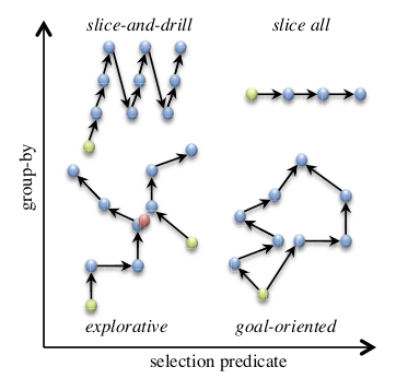
Our first experiments aim at showing that the belief probability distribution learned with our approach is coherent with what could be expected in realistic exploration situations. To settle such experiments, we envision two distinct use cases. First, we consider an ideal environment where all explorations are already categorized into several prototypical user profiles that could be used to bias our model. To this aim, we use the CubeLoad generator [26] which 4 exploratory templates, illustrated in Figure 4, will serve as user profiles.

Second, we use real explorations over an open dataset, called the DOPAN workload from now on, where users investigates about energy vulnerability in French Région Centre Val de Loire. We expect these explorations to be more complex and potentially noisy because of queries that are more or less related to the task at hand. This dataset was used in our former work [12], where an expert classified each users’ exploration based on their skill expertise.

For each use case, several simulations are conducted to assess that our learned probability distributions behave differently and accordingly to what was expected. This section first introduces the experimental protocol for each use case in Section 6.1, proposes some hypothesis about the expected results in Section 6.2 and finally describes and analyses the results in Section 6.3.

Figure 4: Exploration templates in CubeLoad (from [26]): , “seed queries in green, surprising queries in red”.

6.1 Experimental protocol

Evaluation of quality

We will establish our results around two distinct evaluation methods:

1. we run a quantitative evaluation that relies on a distance between two probability distributions: the goal is to estimate to which extent they are close and behave similarly. A classical choice could have been to use a Kullback-Leibler divergence, but here we prefer to use the discrete Hellinger distance that has the advantage of being symmetric and bounded in the interval $[0,1]$. The discrete Hellinger distance $H(P,Q)$ compares two discrete probability distributions $P=(p_{1},\ldots,p_{k})$ and $Q=(q_{1},\ldots,q_{k})$ as follows:

   $$H(P,Q)=\frac{1}{\sqrt{2}}\sqrt{\sum_{i=1}^{k}(\sqrt{p_{i}}-\sqrt{q_{i}})^{2}}$$ (5)

2. we run a qualitative evaluation based on a comparison of plots of average probability distributions presented in decreasing order. Here, we do not look at a direct comparison of estimated probabilities for a given query part, but we are rather interested in the overall shape of the belief distribution and noticeably how the probability decreases and the long tail behavior.

Implementation

Our approach is implemented in Java using jaxen to read cube schemas and Nd4j for simple and efficient matrix computation. The code is open source and available in a GitHub public repository.

6.1.1 CubeLoad use case

We generated a series of 50 explorations using the Cubeload generator over the schema of a cube constructed using the SSB benchmark [24], that we split in 2 groups: the first 43 explorations are used to construct the topology graph, and the next 7 are taken from a single CubeLoad template, and are used to define the user profile. We run 50 randomized samples to achieve a traditional cross-validation protocol.

6.1.2 DOPAN use case

The DOPAN workload contains $32$ explorations in total, that have been authored by $10$ master students of a Business Intelligence program. DOPAN contains 3 data cubes with, respectively, 19, 14, and 27 dimensions, and 32, 20, and 58 measures. We expect this dataset to be more challenging than CubeLoad since real users are likely to be less predictable than simulated ones with potential erroneous queries during the exploration. Interestingly, users’ explorations are categorised according to the skill expertise in $3$ groups: $B$ users are the less experienced, $C$ users show average skills while $D$ users are supposed to write the most appropriate queries. Noticeably, this dataset’s noise and longer explorations can be explained by the behavior of OLAP tools, like Saiku, as they log a new query for each user action (including intermediate drag-and-drops).

6.2 Hypothesis

6.2.1 CubeLoad use case

We expect the 4 templates included in CubeLoad to behave differently. The slice all template is a local user model that only explores a small fraction of the data space. It is thus expected that when comparing to a baseline distribution probability agnostic of any user specific graph, it will maximize this distance. In this case, only a few query parts concentrate most of the interactions with a higher probability, as all queries of the exploration share the same group by set and measure. Similarly, as the slice all template chooses one level in one hierarchy and then only varies the selection predicate, it is expected to show a larger standard deviation than the other templates from one exploration to the next.

On the contrary, the explorative template simulates a broader exploration of the data space. This template should lead to minimizing its distance with a topology based distribution. In this case, it is expected that there are fewer very improbable query parts but that there are more higher probabilities on most query parts, because of the coverage of the data space by the template.

The goal-oriented and slice-and-drill templates are expected to be intermediate states between the two previous templates. Indeed, both models explore the data space more than slice-all, but are a bit more constrained than explorative.

6.2.2 DOPAN use case

The DOPAN use case is more complex since it deals with real explorations for which we do not know the profile of the users, contrary to CubeLoad. We expect these experiments to confirm the tendencies observed in the CubeLoad dataset, with an ability of our belief distribution to capture the knowledge of the users. However, we expect these results to be less contrasted than what is observed for CubeLoad for two reasons: ($1$) the cubes in DOPAN are more complex in terms of schema ($2$) the users in the experiments were all trained in the same master program and thus should exhibit some common behviours , which may not help distinguishing from one profile to the next.

6.3 Results

6.3.1 CubeLoad use case

Table 1 represents the distance between:

• the PR vector computed over the topology graph $G_{t}$ (see Section 4),

• and the PR vector computed over the aggregated graph as produced by Algorithm 3, that merges the topology graph $G_{t}$ with the user specific graph $G_{u}$. In order to bias our model, we gradually modify the parameter $\alpha\in[0,1]$ of the merge function in Algorithm 3 to give more importance to $G_{u}$ compared to $G_{t}$.

User/$\alpha$	0.1	0.2	0.3	0.4	0.5	0.6	0.7	0.8	0.9
Explorative	0.021	0.042	0.063	0.084	0.106	0.130	0.155	0.183	0.215
Goal Oriented	0.015	0.031	0.047	0.063	0.081	0.101	0.123	0.150	0.182
Slice All	0.073	0.127	0.170	0.209	0.244	0.279	0.315	0.350	0.392
Slice and Drill	0.022	0.044	0.066	0.089	0.114	0.139	0.167	0.200	0.236

Table 1: Average Hellinger distance between the topology graph PR and the user-specific graph PR, following the templates of CubeLoad (std. dev. on the order of $10^{-3}$ no represented here)

Table 1 details the Hellinger distance values computed between the two PR’s, for each of the 4 CubeLoad templates, and values of parameter $\alpha$ ranging from $0.1$ to $0.9$. The first observation from Table 1 is that Cubeload profiles indeed differ in how close they are to the reference distribution. This means that different user activities can be characterized to correspond to different belief by our approach. We can also observe that the distance between the resulting distributions is proportional to $\alpha$ as expected. Indeed, if $\alpha$ is very low, the biased distribution is very close to the PR topology distribution. The higher $\alpha$, the more characteristics from the user profile are introduced in the transition matrix. Second, and as expected, we notice that the slice-all profile bears the larger distance with the topology as it only explores a small portion of the possible space, while the other profiles seem to have a comparable behavior in terms of distance. It can be observed that goal-oriented profile tends to generate the lowest distances to the PR that represents the topology graph. This can be explained by the fact that goal-oriented is somehow the less constrained simulated user profile as it mainly performs a random walk in the topology graph to a destination query following the schema. In contrast other profiles and noticeably slice-all and slice-and-drill restrict more strongly their explorations of the graph to fixed patterns that may contradict probabilities of transitions as observed in most past usages and schema.

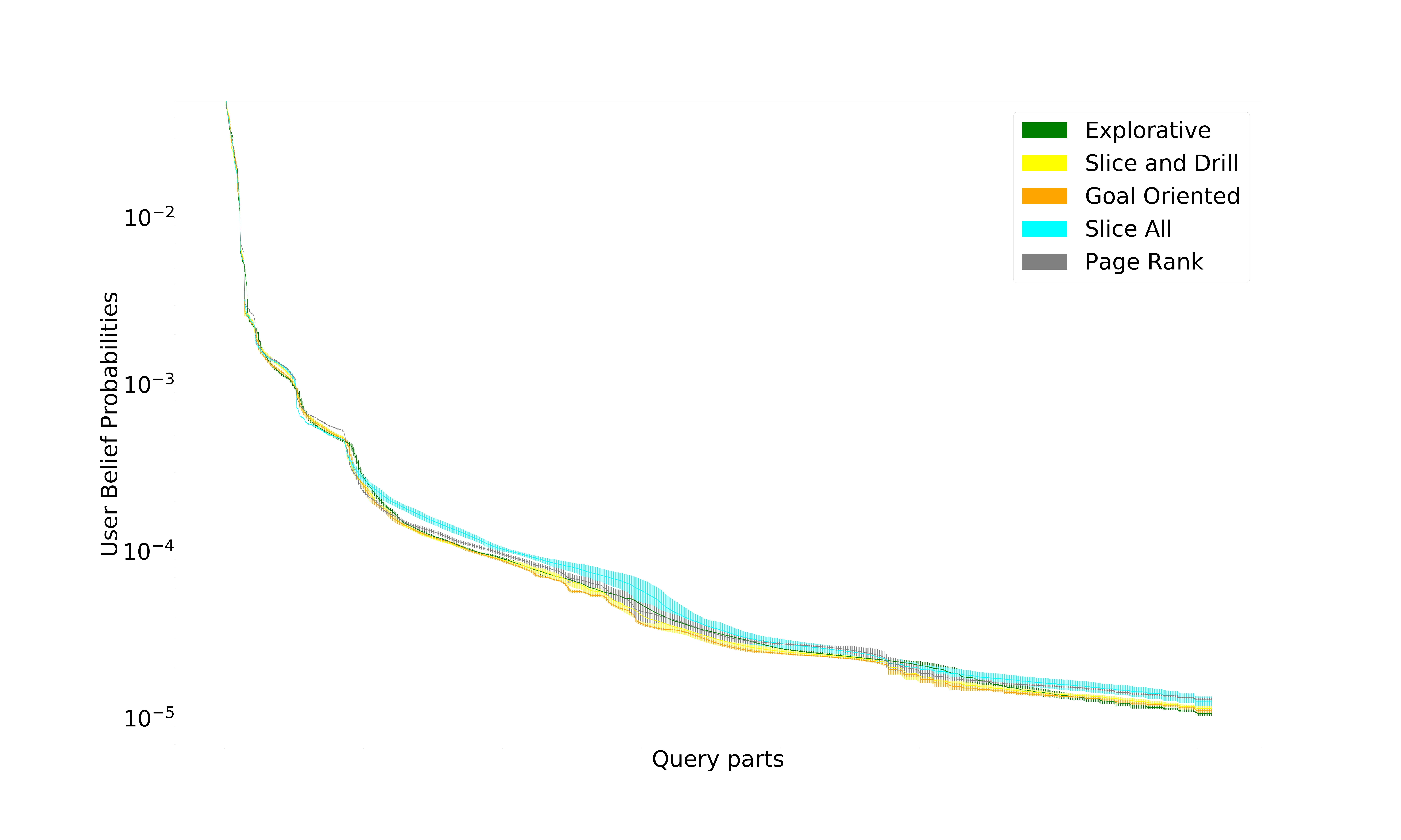
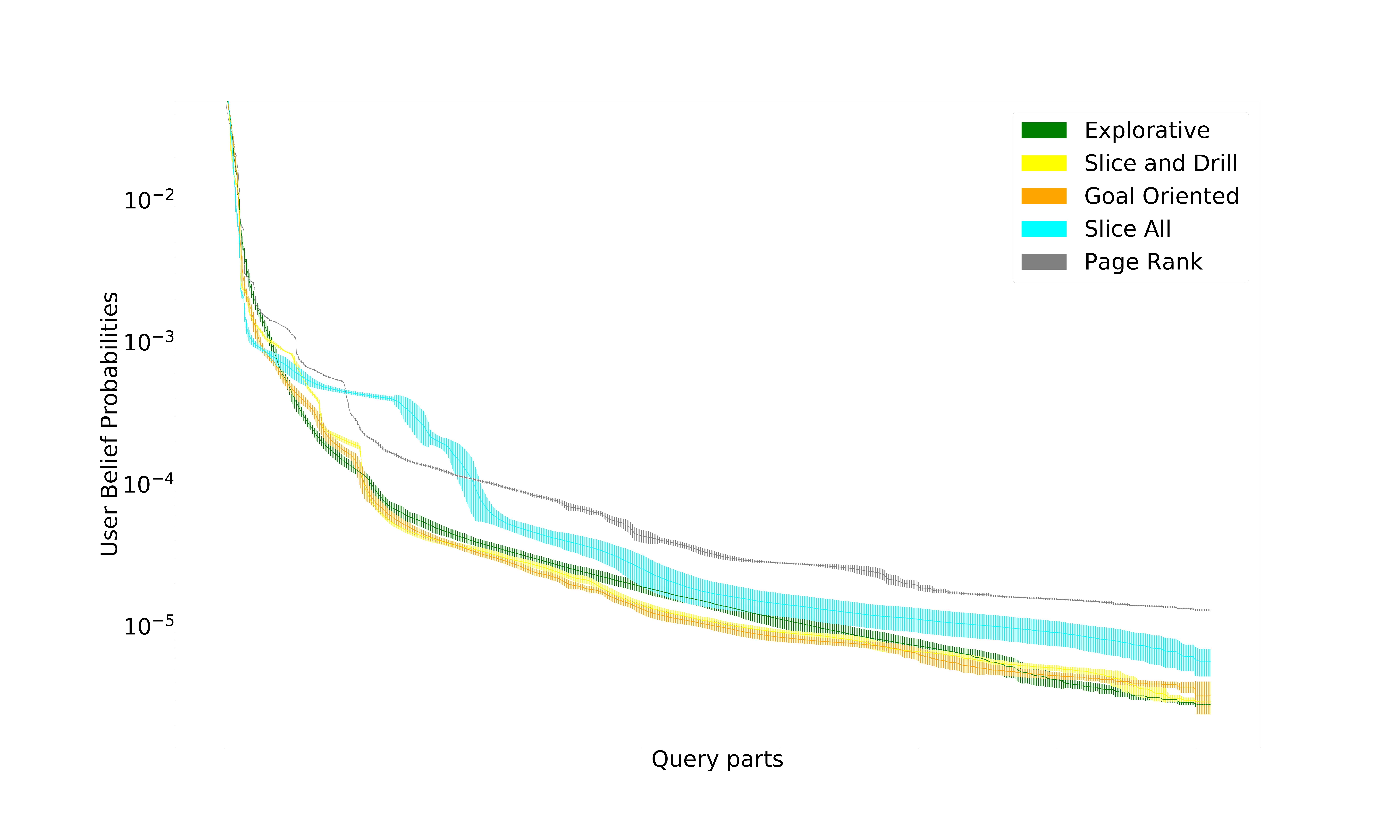
Figures 5 and 6 represent, for two distinct values of parameter $\alpha$, the average distribution of probabilities (and their standard deviation) for the $4$ user profiles and the PR distribution corresponding to the topology averaged on 200 tests. As expected, when $\alpha=0.2$ all distributions heavily tend to mimic the PR distribution. On the contrary, when $\alpha=0.8$ the difference brought by the user profile become clearly visible. The slice-all profile tends to have a higher number of higher probabilities and then decreases with successive steps which are characteristic of this profile. Indeed, this profile explores all members at a given depth in a hierarchy and all the corresponding query parts are by construction almost equiprobable: only past usage may modify probability which translates in the observed decrease pattern. Then, as expected the slice-all profile shows the largest standard deviation in our test, which can be explained by the variability of each exploration from this profile that explore each time a different hierarchy at a different level.

Similarly, slice-and-drill profile exhibits some small but noticeable steps that can be explained by the fact that this profile alternatively navigate between members of a hierarchy at a given level and at some point drill down to query parts from lower level of the hierarchy and that are less likely to be used, as they are more specialized and thus less probable.

Then, it is worth noticing that the PR plot also shows some steps which may traduce the presence of more strongly connected components inside the topology graph where query parts are equiprobable.

Finally, explorative and goal-oriented profiles exhibits a more gradual decrease of the probabilities which is again expected as these approaches distributes more evenly their probabilities into more query parts because of their behavior.

Figure 5: Distribution of probabilities computed by our model for all $4$ user profiles when $\alpha=0.2$ (log scale). Each plot represents the probabilities of the query parts for one user profile in decreasing order

Figure 6: Distribution of probabilities computed by our model for all $4$ user profiles when $\alpha=0.8$ (log scale). Each plot represents the probabilities of the query parts for one user profile in decreasing order.

6.3.2 DOPAN use case

User/$\alpha$	0.2	0.8
User 03	0.00134	0.0586
User 04	0.00417	0.135
User 05	0.000565	0.00244
User 06	0.00201	0.0692
User 07	0.00560	0.150
User 09	0.00423	0.131
User 10	0.00367	0.133
User 12	0.0000244	0.00134
User 14	0.00567	0.136
User 16	0.00530	0.151

Table 2: Hellinger distance between PR and our biased PR with several user profiles on the DOPAN dataset

Similarly to Table 1, Table 2 indicates the distances between the PR topology distribution and distributions obtained by biasing the topology graph with users explorations on the DOPAN cubes. For the sake of simplicity, Table 2 only presents the Hellinger distances computed for 2 distinct values of parameter $\alpha$ that are either topology oriented ($\alpha=0.2$) or user oriented ($\alpha=0.8$).

It can be first noticed that the distance values are much smaller than in the case of CubeLoad explorations as expected. This is explained by the higher complexity of the DOPAN cubes combined with fewer explorations per user, in contrast to the CubeLoad experiments that were conducted with more explorations over a simpler SSB cube. This indicates that our modeling of belief therefore correctly accounts for the complexity of the query space.

Noticeably, two users exhibit very low distances to the reference belief. By manually reviewing those user logs we observed that they had very short explorations compared to the other users. As a consequence, a small user log will not change much the aggregated graph when mixed with the topology graph and therefore have almost no influence on the PR vector and on the computed distances. In other words, the probability to use a specific query part for a user with little experience is dictated by the schema and general user navigational habits.

Figure 7: Distribution of probabilities over the first (and most used) cube of the DOPAN dataset. Query parts are ordered according to their decreasing probability value for each student. Note that the plot has been limited to the first $3000$ queries for the sake of readability.

In Figure 7 we display in the same way as Figure 5 and Figure 6 the belief distribution of the user but here on the real explorations over the first cube of the Dopan dataset. Interestingly, we can observe that student $14$ behavior is reminiscent to the behavior exhibited by CubeLoad’s Slice All profile. By reviewing the user’s explorations we found that they change the selection predicate over several queries while keeping measures and group by set elements from previous queries. This behavior is very similar to the one described by a Slice All pattern, and indicates that our modeling of belief can help differentiating specific ways of exploring.

7 Exploration evaluation based on Subjective Interestingness

We use Algorithm 4 to compute the subjective interestingness (SI) on the explorations of our two datasets. The aim of these tests is to show how SI relates to prototypical user behaviors (Cubeload use case) and to real user explorations (DOPAN use case). We start by describing the protocols for the two use cases and then comment our experimental results.

7.1 Experimental protocol

In both use cases, we use $\alpha=0.9$ for Algorithm 4 to compute the SI incrementally for each explorations, to better account for the user (simulated or real) behavior. We now explain the difference in protocol for the two uses cases.

CubeLoad

Explorations generated with CubeLoad correspond to prototypical behaviors (profiles) of users navigating a datacube. For our first experiment, we generate $50$ explorations for each different CubeLoad profile. We first plot the accumulated number of unique query parts used at each moment of the exploration to understand how our complexity measure behaves. We then run Algorithm 4 on each explorations to compute the subjective interestingness per query. For each profile, we isolate the current explorations from the others generated. All the other explorations of the same profile will be used as a user past log. The results are finally aggregated per profile and query position in the exploration, to compute the mean and the standard deviation of SI. We display the results in the form of a line plot with error bars representing the standard deviation. The query position on the $x$ axis represents different moments of the exploration. Each line is a cubeload profile representing the mean behavior of all explorations generated using this profile. Our aim is to see how SI behaves along the explorations and allows to characterize the prototypical profiles.

DOPAN

For the DOPAN use case, we have at our disposal $32$ real user explorations. We will focus on the 22 explorations over the first cube of DOPAN, since SI cannot be compared across cubes with different schemas. Contrary to the simple SSB cube, that one has 32 measures and 19 dimensions, making it a much larger space to explore. Our protocol is a bit different than the one used for CubeLoad since we have not classified the explorations in how they follow a particular pattern. However, each exploration has been tagged by professors with labels B, C or D, depending on analyst’s skills. Label D corresponds to good explorations, clearly following an information need, investigating it and containing coherent queries. Students producing such explorations are considered to have analysis skills. Contrarily, label B denotes those of the students that produced poor explorations, with less contributive queries, typically switching topics, with no clear information need. Label C corresponds to students that are learning analysis skills, but still produce middle-quality explorations.

Like for the CubeLoad use case, we first plot the accumulated number of unique query parts used at each moment of the exploration. We run Algorithm 4 on each exploration to compute SI per query, using, for the user history to build $G_{s}$, an exploration consisting of the past queries of the exploration and, whenever possible, the queries of other explorations of that user. Note that users have done different number of explorations, each of different sizes, and therefore our protocol faithfully represent genuine user activities. We use the same line plot as for CubeLoad to show the SI of each query of the explorations, to analyze how SI varies in the exploration and detects instantaneous analysis behavior. We then group explorations per skill labels and plot the mean and confidence interval at 95% of SI for the 3 groups, again with line plot. We finally compute the rank correlation between SI and the skill.

7.2 Results

7.2.1 CubeLoad use case

Figure 8: Cumulated number of unique query parts by CubeLoad template for each query index in the explorations

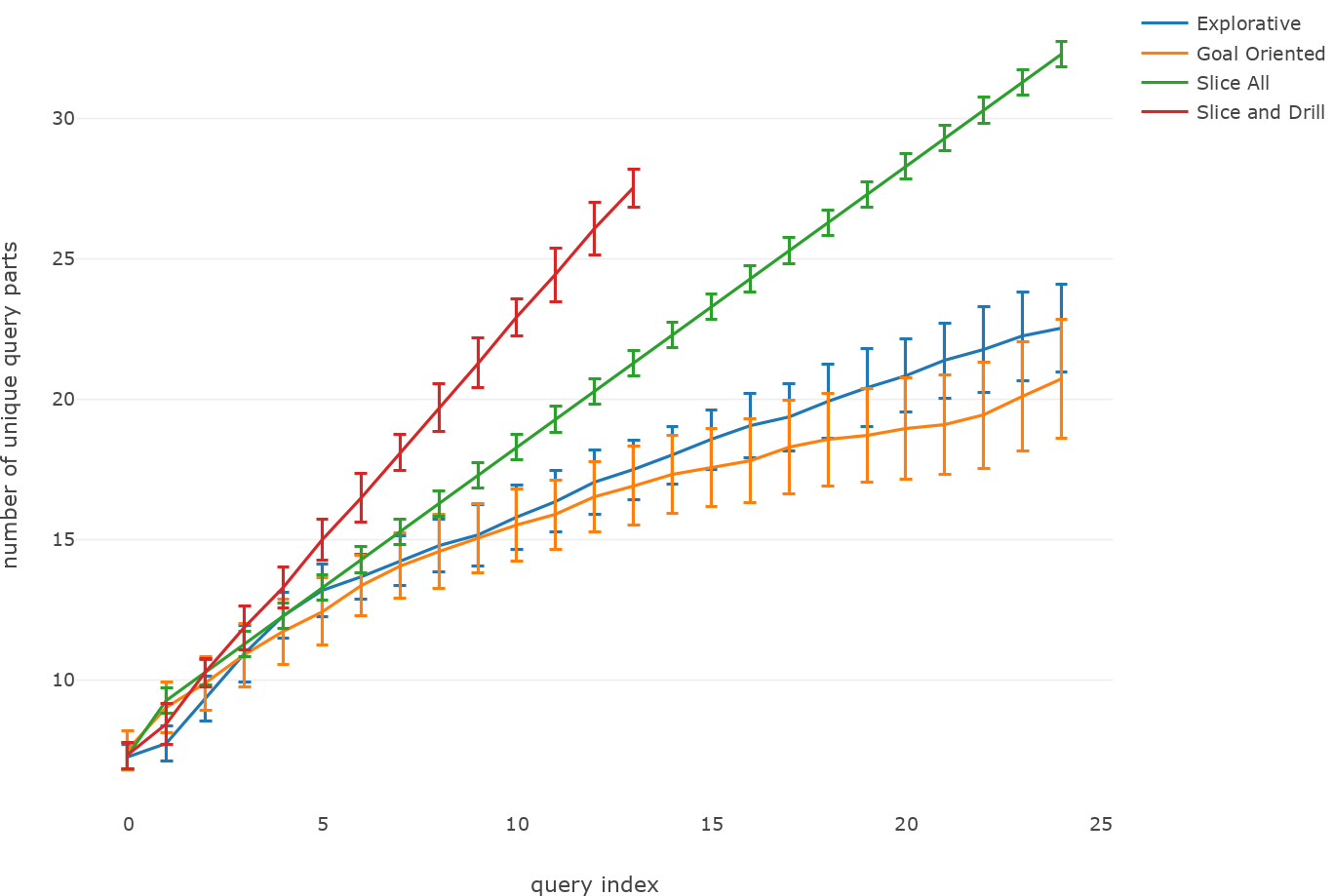
Figure 8 shows the accumulated number of unique query parts used at each moment of the exploration. This measure increases monotonically since each newly generated query adds one or more parts, some being already seen and counted, allowing to rank the 4 profiles. As expected, the slice and drill profile generates the more never encountered query parts since this pattern necessarily goes in one new direction, either by drilling or slicing. It is followed by the slice all pattern, that only add new slices. Then comes the two profiles that are constrained by either a goal query (goal oriented) or a ”surprising” query (explorative), and as such may not necessarily add never seen query parts since they are forced to stay around those queries. The goal oriented has a bit less new query parts since it is constrained all along the exploration, while explorative is only constrained half of it.

Figure 9: Subjective Interestingness for each cubeload profile

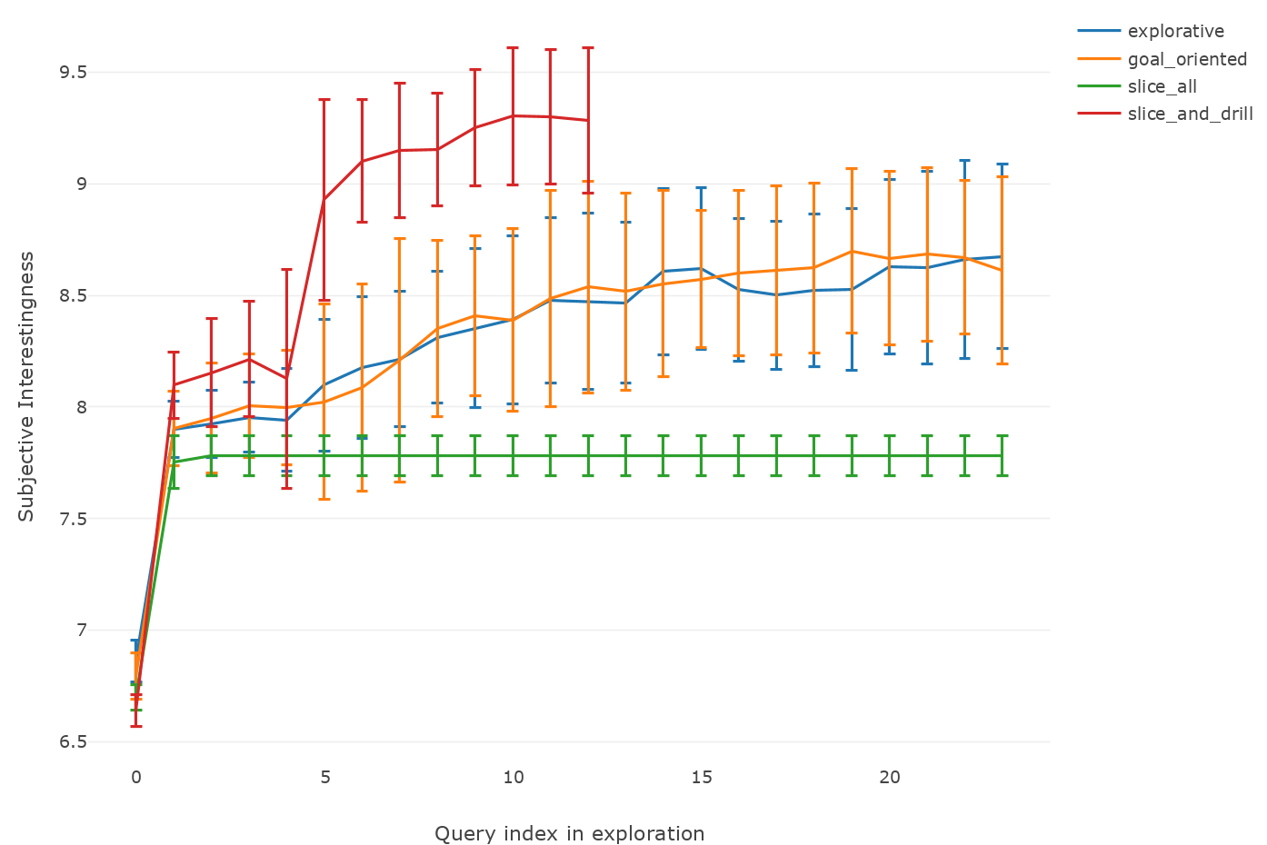
As can be observed in Figure 9, SI is capable of discriminating the cubeload profiles, except for the goal oriented and explorative profiles that cannot be distinguished. This behavior is expected since both profiles exhibit changes to selection and group by attribute at each query. Both behaviors will therefore generate quite large amounts of information and thus will hardly be distinguished with SI.

The slice all profile shows the least amount of Subjective Interestingness because of the way its queries are generated. At each step, the query parts are very minimally altered, thus generating less surprise while keeping a constant query complexity. The combination of these two behaviors cause the Subjective Interestingness to be almost constant across all queries of an exploration for this profile. The slice and drill profile is clearly the profile generating the most subjectively interesting queries. Compared to the other profiles, slice and drill generates the greater variety of query parts since it systematically moves by using new query parts, without remaining at the same group by level (like slice all) and without being attracted to some queries (like explorative or goal oriented). Being both constrained, albeit not in the same way, explorative and goal oriented profiles exhibit an intermediate behavior and cannot be easily distinguished with SI.

7.2.2 DOPAN use case

Figure 10: Cumulated number of unique query parts by skill for each query index in the explorations.

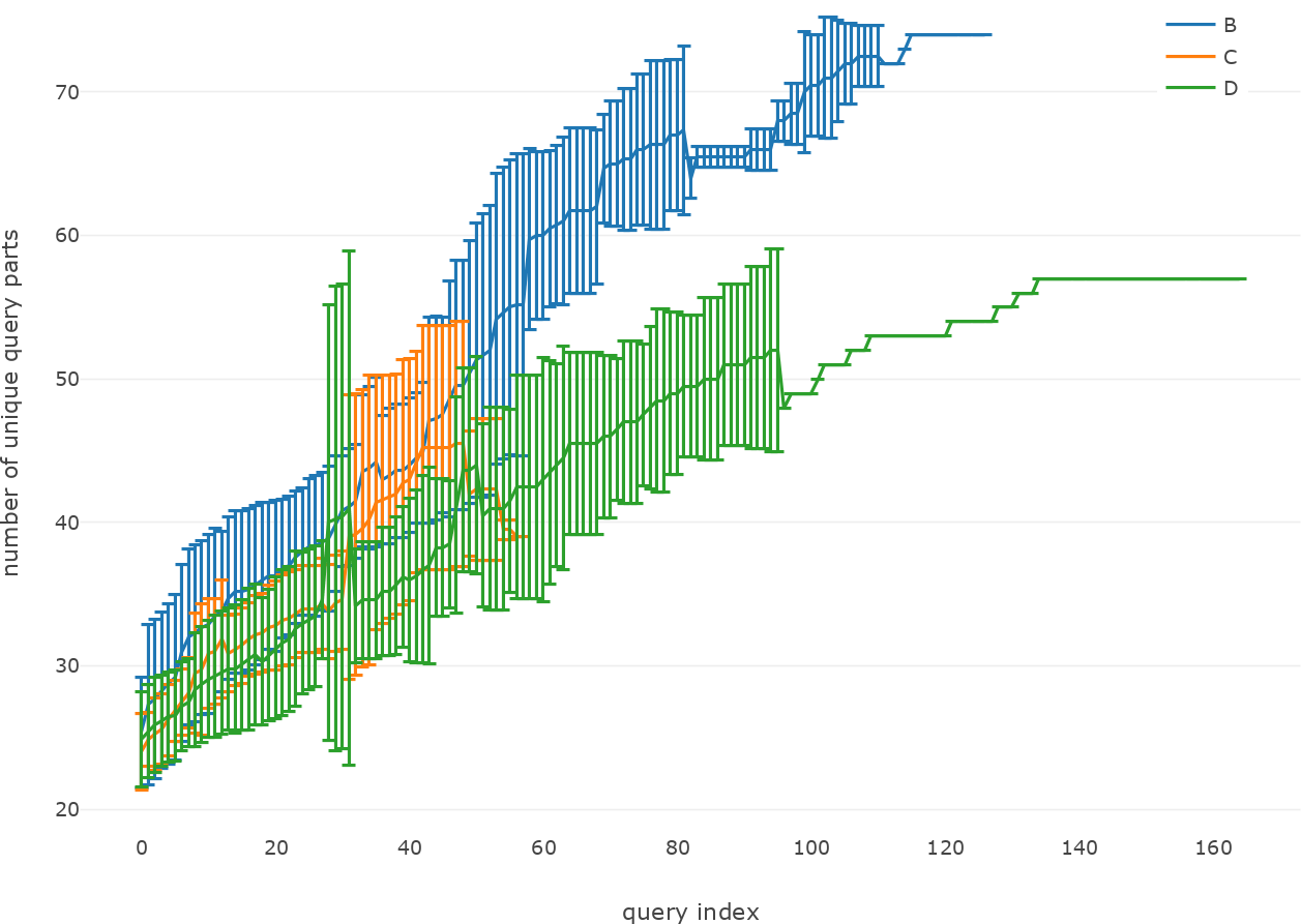
Figure 10 plots the cumulated number of unique query parts by skill (B, C or D) for each query in the explorations. Clearly, B labelled explorations have more never seen new query parts, while D labelled explorations have less never seen query parts. The increase rate is also more pronounced for B explorations, and higher than for D explorations. This is explained by the fact that lower skill explorations exhibit a more explorative and erratic behaviour that periodically tries new directions to explore. Manually reviewing the B explorations, we indeed have found that their behavior is sometimes reminiscent of the slice and drill profile described in Figure 4. On the contrary, D labelled explorations tend to produce less query parts, since these explorations exhibit the behavior of a user knowing how to formulate efficiently minimal queries to get to their objective.

Category C explorations have a mixed behavior with a similar behavior as category D at the beginning and then gradually converging to a situation where they produce as many query parts as the beginner explorations. Interestingly, category C also produces shorter explorations, as shown in Figure 10, as these explorations were deemed to be executed by a ”user acquiring analytically skills” ; they will choose useful measures, use relevant selection predicates but their explorations might be cut short because they did not manage to answer a business questions or did not go the extra step to understand discrepancies in the data they find (e.g., by drilling down). Finally, Figure 10 reflects with the cumulated number of query parts, the spread of each exploration skill profile in our query parts graph, which directly impacts our Subjective Interestingness measure.

Figure 11: Average and confidence interval of SI by skill for each query index in the explorations (top left), SI for all explorations of skill B (top right), C (bottom left) and D (bottom right), each color being an individual exploration.

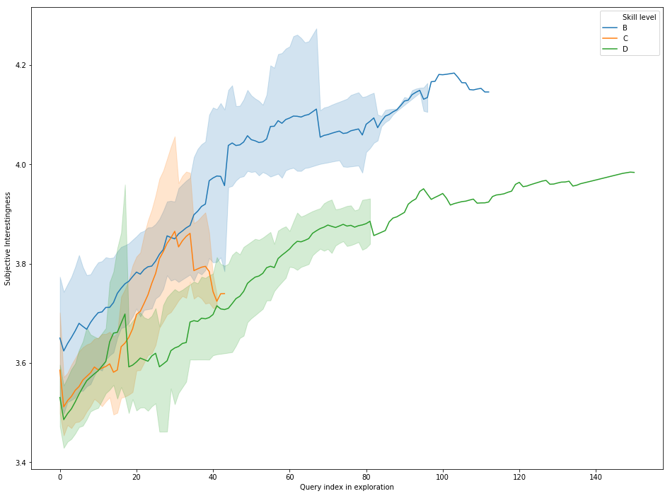
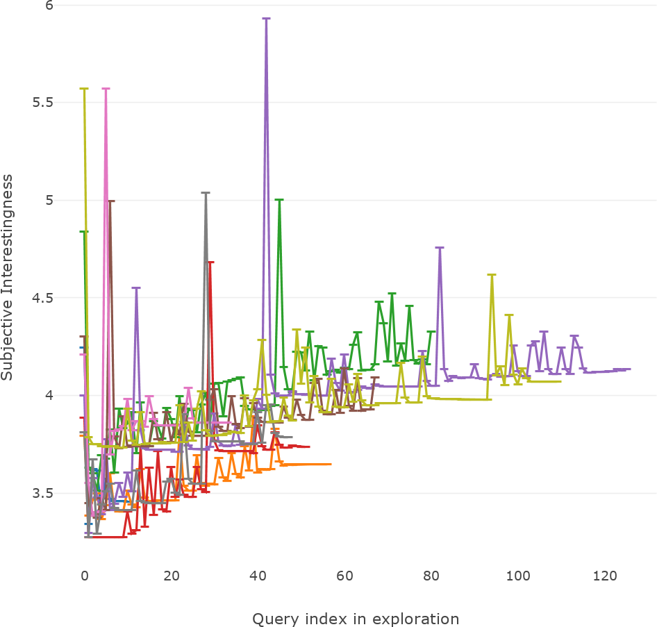
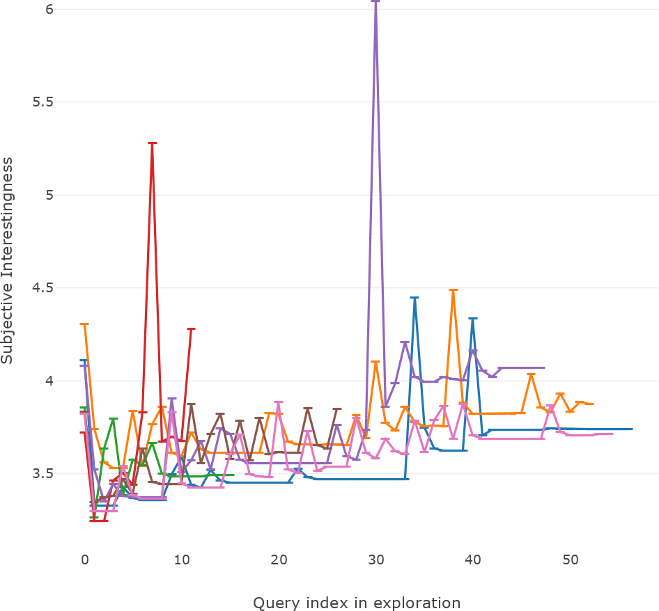
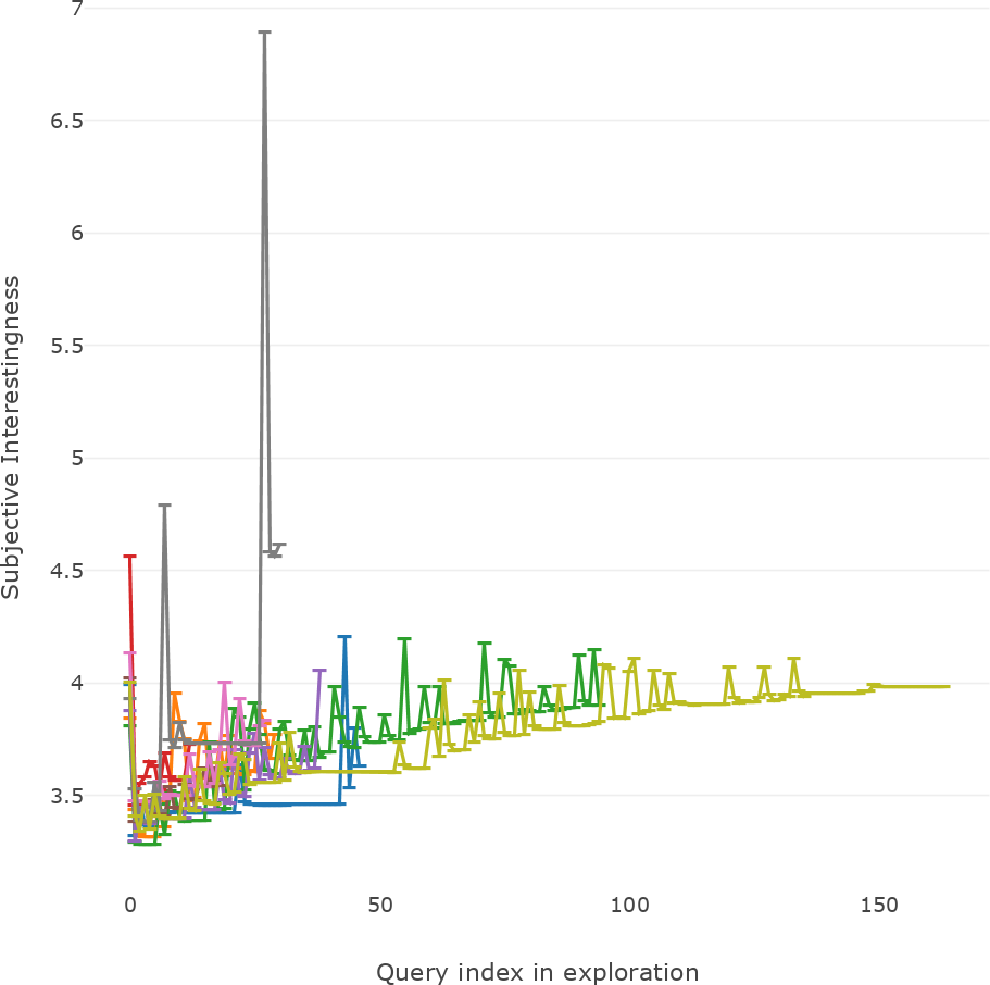
Figure 11 (top left) shows the average SI with confidence interval of each query of the explorations, grouped by skill labels and presented by query position in the exploration. Noticeably, SI characterizes B labelled explorations with the highest average score and D labelled explorations with the lowest, while C labelled explorations are in between. High SI corroborates the explorative nature of B explorations, where users struggle to find their way in the multidimensional space by selecting unseen query parts somewhat erratically. On the contrary, low SI corroborates the more ”focused” nature of D explorations, where users are more pragmatic in their choice of query part to express classical OLAP operations like roll-up or drill-down. Doing such choices, i.e., selecting query parts close to the ones already employed mechanically lowers SI, since the belief attached to those new parts is high and therefore their surprise is low. Regarding C explorations, they were labelled a such because they exhibit behaviors coming partly from unskilled explorations and partly from skilled ones. While SI is not conceived to discriminate user skills, it can still position those intermediate behaviors between the two extremes.

Figure 11 (top right and bottom) shows the SI for the queries of each exploration, separated by skills. It is immediately noticeable that there are sudden and short spikes in the SI. By looking at the specific queries where those spikes occur, we could see that the users suddenly add large numbers of selection predicates. By design, our measure can detect such behaviors since adding a high number of parts, even if they have a high probability of being selected, result in high SI due to how probabilities are used to compute surprise (see equation 4) and because of the sudden increase in the complexity of the query. The queries obtained with such a burst of new query parts are likely to be informative and correctly detected by our measure.

Finally, we have validated these observations with a rank correlation test between skills (B, C, D) and the Subjective Interestingness measure that outputs a score of $-0.28$. This result confirms that there is a correlation between the skill category and our Subjective Interestingness Measure: the lower the category, the higher the Subjective Interestingness.

8 Related Work

Our work deals with subjective interestingness and how to define such a measure by learning a belief distribution from users’ past activities in the context of Business Intelligence. This section presents some interestingness measures, and how they have been used in the context of recommendation and exploratory data mining.

Defining a good Interestingness measure has kept interested researchers for a long time in the context of data mining. Indeed, there exists numerous tasks, for example in pattern mining, for which it is critical to be able to filter out uninteresting patterns such as item sets or redundant rules, to control the complexity of the mining approaches and increase their usability.

In [8, 16], the authors identify two main types of interestingness measures. Objective measures are based only on data, which corresponds to quality metrics such as generality, reliability, peculiarity, diversity and conciseness. For instance, directly measurable evaluation metrics such as support confidence, lift or chi-squared measures in the case of association rules [3].

On the contrary, subjective measures consider both the data and the user and characterize the patterns’ surprise and novelty when compared to previous user knowledge or expected data distribution. The first work on the topic of subjective interestingness is certainly [30] that is restricted to the pattern mining domain. In [5, 7], the author extends this notion to any explorative data mining task and represents interestingness as a ratio between information content and complexity of a discovered pattern being it an itemset, a cluster or a query evaluation result (see Section 3.2 for more formal details). In [7], De Bie defines the subjective interestingness as a situation where a

“user states expectations or beliefs formalized as a ‘background distribution’. Any ‘pattern’ that contrasts with this and is easy to describe is subjectively interesting”.

The authors in [16] consider also semantic measures of interestingness, based on the semantics and explanations of the patterns like utility and actionability. This latter property of actionability is not meaningful in our case where, as stated by De Bie [7], we consider situations

“where the user is interested in exploring without a clear anticipation of what to expect or what to do with the patterns found”.

De Bie’s framework [5] is usually used to model user belief about some data. The hypothesis is that the user has beliefs about all of the data and is interested by anything that is surprising according to her beliefs. This will usually be a piece of data whose properties greatly contradict the user’s prior belief. This work is very similar to what Sarawagi did for multidimensional data exploration [29]. In her work, the user’s previous observations about parts of the data is used to estimate the most probable cube instance in the user’s brain. A dissimilarity to the actual cube instance data is then computed in order to recommend surprising subsets. Both approaches compute a kind of information gain conditioned by the knowledge of what has been seen by the user while he explored the data. This gives the system the ability to suggest the best action that will provide the most information out of the data to the user.

Modelling the probability over the user intents would be another subjective approach. This is well illustrated by the Bayesian Information Gain method, as shown in various works by Wanyu [23] for instance. With this approach, the system makes hypothesis about the user’s goal and test them by subjecting her to experiments. The goal is to find the experiment which would yield most information about the user’s goal to the system, to help her reach it faster. Both approach seems quite complementary as De Bie’s approach makes possible query recommendation through interesting data discovery and Wanyu’s approach instead allows similar recommendation through intent discovery. Interestingly, these intents are probability distribution over elements of knowledge, while other works have focused on capturing long or short term intents related to topics for data exploration such as [14].

Recently, in [25] the authors propose a data exploration study based on De Bie’s FORSIED framework [6, 7] that pairs a high level conjunctive query language to identify groups of data instances and expresses belief on some real-valued target attributes, based on location and spread patterns. This work is close to our proposal but expresses belief on a summary of the data.

In general, most of recent work on De Bie’s framework [22, 31] instantiate his framework to discover subjectively interesting pattern for different kind of data spaces. As a consequence, papers detail new pattern syntax as well as other statistics computed on the pattern extension. For example, in [31], De Bie’s uses his framework to find subjectively interesting dense graph patterns: each pattern is a set of nodes and the statistic is the average degree of the edges in the pattern’s nodes. In [22], the pattern used are subgroups of instances described by conjunctions of categorical descriptive attributes, while the statistics are the mean and the covariance of the subgroup for any number of real-valued target attributes.

In the context of data cube exploration, to the best of our knowledge there is no final and consensual interestingness measure or belief distribution elicitation method, while there exists measures that are closely related. Measures have been defined as unexpectedness of skewness in navigation rules and navigation paths [21] and computed as a peculiarity measure of asymmetry in data distribution [19]. In [15], the authors define interestingness measures in a data cube as a difference between expected and observed probability for each attribute-value pair and the the degree of correlation among two attributes. In [28], Sarawagi describes a method that profiles the exploration of a user, uses the Maximum Entropy principle and the Kullback-Leibler divergence as a subjective interestingness measure to recommend which unvisited parts of the cube can be the most surprising in a subsequent query.

In [12, 13] the authors use supervised classification techniques to learn two interestingeness measures for OLAP queries: ($1$) focus, that indicates to what extent a query is well detailed and connected to other queries in the current exploration and ($2$) contribution that indicates to what extent a query contributes to the interest and quality of the exploration.

Finally, interestingness and related principles have been studied in the context of recommendation but more widely used for evaluation rather than the recommendation itself [18]. Interestingness is reflected based on $4$ main criteria such as diversity, serendipity, novelty, and coverage, in addition to traditional accuracy measures.

In the context of OLAP query recommendation, several recommendation algorithms have been proposed that take into account the past history of queries of a user either based on a Markov model [27] or on extracted patterns [2]. Noticeably, [2] quantifies how distant is the recommendation from the current point of exploration to evaluate the interestingness of each candidate query recommendation.

9 Conclusion

This paper addresses the question of determining what is interesting for a specific user during an interactive exploration of a multidimensional cube. To that extent, the paper draws a parallel with De Bie’s Forsied framework [5], and defines a subjective interestingness measure for a query as a ratio between the surprise expressed through this query and its complexity. Defining such a measure raises $3$ main challenges: ($1$) how to model and learn the prior user belief as a probability distribution to model surprise? ($2$) How to efficiently recompute this prior belief after each user query? And, ($3$) how to implement a realistic Subjective Interestingness measure that captures the complexity of each query?

Our measure definition takes advantage of the specificities of Business Intelligence explorations of multidimensional data cubes. We represent the prior knowledge of a specific user as a directed graph of query parts that relies: on former users’ explorations, as a proxy of what the current user might find interesting, on the cube schema, that indicates how prior knowledge is structured, and finally on this specific users’ past activity. Finally, the user belief is derived from this query parts graph as the stationary probability distribution of a PageRank algorithm. Experiments conducted on simulated realistic user explorations or on real user explorations show that the observed belief distribution and subjective interestingness values are aligned with prior knowledge on these datasets. This first work on the definition of a subjective interestingness measure in Business Intelligence shows that query parts offer a reasonable proxy to learn an appropriate model of user belief and determine what is interesting in an exploration.

However, in De Bie’s framework, the belief is expressed on the extension of the data and not on the intention of the way of characterizing the data subgroup. A first major extension to our work will consist in proposing a belief and subjective interestingness measure on the value of each cube cells. Second, we plan to investigate how to define such an interestingness measure for less structured databases, like relational (non multidimensional) databases, or data lakes. Finally, we aim at studying how user belief modeling and subjective interestingness measures combine with higher level intentional languages to query and learn from the data [32].

References

- [1]
- Aligon et al. [2015] Julien Aligon, Enrico Gallinucci, Matteo Golfarelli, Patrick Marcel, and Stefano Rizzi. 2015. A collaborative filtering approach for recommending OLAP sessions. DSS 69 (2015), 20–30.
- Alvarez [2003] S. Alvarez. 2003. Chi-squared computation for association rules: preliminary results. Technical Report BC-CS-2003-01. Computer Science Dept. Boston College, Chestnut Hill, MA 02467 USA. 11 pages. http://www.cs.bc.edu/~alvarez/ChiSquare/chi2tr.pdf
- Bie [2011] Tijl De Bie. 2011. An information theoretic framework for data mining. In KDD. ACM, 564–572.
- Bie [2013] Tijl De Bie. 2013. Subjective Interestingness in Exploratory Data Mining. In Advances in Intelligent Data Analysis XII - 12th International Symposium, IDA 2013, London, UK, October 17-19, 2013. Proceedings. 19–31. https://doi.org/10.1007/978-3-642-41398-8_3
- Bie [2018b] Tijl De Bie. 2014 (accessed on December 2018)b. The Science of Finding Interesting Patterns in Data. http://www.interesting-patterns.net/forsied/
- Bie [2018a] Tijl De Bie. 2018a. An information-theoretic framework for data exploration. From Itemsets to embeddings, from interestingness to privacy. In Keynote presentation given at IDEA’18 @ the KDD’18 conference. http://www.interesting-patterns.net/forsied/keynote-presentation-given-at-idea18-the-kdd18-conference/
- Brijs et al. [2004] Tom Brijs, Koen Vanhoof, and Geert Wets. 2004. Defining Interestingness for Association Rules. International Journal ”Information Theories & Applications” 10 (2004), 370–375.
- Brin and Page [2012] Sergey Brin and Lawrence Page. 2012. Reprint of: The anatomy of a large-scale hypertextual web search engine. Computer Networks 56, 18 (2012), 3825–3833. https://doi.org/10.1016/j.comnet.2012.10.007
- Cariou et al. [2009] Véronique Cariou, Jérôme Cubillé, Christian Derquenne, Sabine Goutier, Françoise Guisnel, and Henri Klajnmic. 2009. Embedded indicators to facilitate the exploration of a data cube. IJBIDM 4, 3/4 (2009), 329–349. https://doi.org/10.1504/IJBIDM.2009.029083
- Chanson et al. [2019] Alexandre Chanson, Ben Crulis, Krista Drushku, Nicolas Labroche, and Patrick Marcel. 2019. Profiling User Belief in BI Exploration for Measuring Subjective Interestingness. In Proceedings of the 21st International Workshop on Design, Optimization, Languages and Analytical Processing of Big Data, co-located with EDBT/ICDT Joint Conference, DOLAP@EDBT/ICDT 2019, Lisbon, Portugal, March 26, 2019. http://ceur-ws.org/Vol-2324/Paper08-PMarcel.pdf
- Djedaini et al. [2019] Mahfoud Djedaini, Krista Drushku, Nicolas Labroche, Patrick Marcel, Verónika Peralta, and Willeme Verdeaux. 2019. Automatic assessment of interactive OLAP explorations. Information Systems 82 (2019), 148–163.
- Djedaini et al. [2017] Mahfoud Djedaini, Nicolas Labroche, Patrick Marcel, and Verónika Peralta. 2017. Detecting User Focus in OLAP Analyses. In ADBIS. 105–119.
- Drushku et al. [2017] Krista Drushku, Julien Aligon, Nicolas Labroche, Patrick Marcel, Verónika Peralta, and Bruno Dumant. 2017. User Interests Clustering in Business Intelligence Interactions. In Advanced Information Systems Engineering - 29th International Conference, CAiSE 2017, Essen, Germany, June 12-16, 2017, Proceedings. 144–158.
- Fabris and Freitas [2001] Carem C. Fabris and Alex Alves Freitas. 2001. Incorporating Deviation-Detection Functionality into the OLAP Paradigm. In XVI Simpósio Brasileiro de Banco de Dados, 1-3 Outubro 2001, Rio de Janeiro, Brasil, Anais/Proceedings. 274–285.
- Geng and Hamilton [2006] Liqiang Geng and Howard J. Hamilton. 2006. Interestingness measures for data mining: A survey. ACM Comput. Surv. 38, 3 (2006), 9.
- Jain et al. [2016] Shrainik Jain, Dominik Moritz, Daniel Halperin, Bill Howe, and Ed Lazowska. 2016. SQLShare: Results from a Multi-Year SQL-as-a-Service Experiment. In Proceedings of the 2016 International Conference on Management of Data (SIGMOD ’16). ACM, New York, NY, USA, 281–293. https://doi.org/10.1145/2882903.2882957
- Kaminskas and Bridge [2017] Marius Kaminskas and Derek Bridge. 2017. Diversity, Serendipity, Novelty, and Coverage: A Survey and Empirical Analysis of Beyond-Accuracy Objectives in Recommender Systems. TiiS 7, 1 (2017), 2:1–2:42.
- Klemettinen et al. [1999] M. Klemettinen, H. Mannila, and H. Toivonen. 1999. Interactive exploration of interesting findings in the Telecommunication Network Alarm Sequence Analyzer (TASA). Information and Software Technology 41, 9 (1999), 557 – 567.
- Kontonasios and Bie [2015] Kleanthis-Nikolaos Kontonasios and Tijl De Bie. 2015. Subjectively interesting alternative clusterings. Machine Learning 98, 1-2 (2015), 31–56. https://doi.org/10.1007/s10994-013-5333-z
- Kumar et al. [2008] Navin Kumar, Aryya Gangopadhyay, Sanjay Bapna, George Karabatis, and Zhiyuan Chen. 2008. Measuring interestingness of discovered skewed patterns in data cubes. Decision Support Systems 46, 1 (2008), 429 – 439.
- Lijffijt et al. [2018] Jefrey Lijffijt, Bo Kang, Wouter Duivesteijn, Kai Puolamäki, Emilia Oikarinen, and Tijl De Bie. 2018. Subjectively Interesting Subgroup Discovery on Real-Valued Targets. In 34th IEEE International Conference on Data Engineering, ICDE 2018, Paris, France, April 16-19, 2018. 1352–1355. https://doi.org/10.1109/ICDE.2018.00148
- Liu et al. [2017] Wanyu Liu, Rafael Lucas D’Oliveira, Michel Beaudouin-Lafon, and Olivier Rioul. 2017. BIGnav: Bayesian Information Gain for Guiding Multiscale Navigation. In Proceedings of the 2017 CHI Conference on Human Factors in Computing Systems, Denver, CO, USA, May 06-11, 2017. 5869–5880. https://doi.org/10.1145/3025453.3025524
- O’Neil et al. [2009] Patrick E. O’Neil, Elizabeth J. O’Neil, Xuedong Chen, and Stephen Revilak. 2009. The Star Schema Benchmark and Augmented Fact Table Indexing. In Performance Evaluation and Benchmarking, First TPC Technology Conference, TPCTC 2009, Lyon, France, August 24-28, 2009, Revised Selected Papers. 237–252. https://doi.org/10.1007/978-3-642-10424-4_17
- Puolamäki et al. [2018] Kai Puolamäki, Emilia Oikarinen, Bo Kang, Jefrey Lijffijt, and Tijl De Bie. 2018. Interactive Visual Data Exploration with Subjective Feedback: An Information-Theoretic Approach. In 34th IEEE International Conference on Data Engineering, ICDE 2018, Paris, France, April 16-19, 2018. 1208–1211. https://doi.org/10.1109/ICDE.2018.00112
- Rizzi and Gallinucci [2014] Stefano Rizzi and Enrico Gallinucci. 2014. CubeLoad: A Parametric Generator of Realistic OLAP Workloads. In Advanced Information Systems Engineering - 26th International Conference, CAiSE 2014, Thessaloniki, Greece, June 16-20, 2014. Proceedings. 610–624. https://doi.org/10.1007/978-3-319-07881-6_41
- Sapia [2000] Carsten Sapia. 2000. PROMISE: Predicting Query Behavior to Enable Predictive Caching Strategies for OLAP Systems. In DaWaK. 224–233.
- Sarawagi [2000] Sunita Sarawagi. 2000. User-Adaptive Exploration of Multidimensional Data. In VLDB. Morgan Kaufmann, 307–316.
- Sarawagi [2001] Sunita Sarawagi. 2001. User-cognizant multidimensional analysis. VLDB J. 10, 2-3 (2001), 224–239. https://doi.org/10.1007/s007780100046
- Silberschatz and Tuzhilin [1995] Abraham Silberschatz and Alexander Tuzhilin. 1995. On Subjective Measures of Interestingness in Knowledge Discovery. In Proceedings of the First International Conference on Knowledge Discovery and Data Mining (KDD-95), Montreal, Canada, August 20-21, 1995. 275–281. http://www.aaai.org/Library/KDD/1995/kdd95-032.php
- van Leeuwen et al. [2016] Matthijs van Leeuwen, Tijl De Bie, Eirini Spyropoulou, and Cédric Mesnage. 2016. Subjective interestingness of subgraph patterns. Machine Learning 105, 1 (2016), 41–75. https://doi.org/10.1007/s10994-015-5539-3
- Vassiliadis and Marcel [2018] Panos Vassiliadis and Patrick Marcel. 2018. The Road to Highlights is Paved with Good Intentions: Envisioning a Paradigm Shift in OLAP Modeling. In Proceedings of the 20th International Workshop on Design, Optimization, Languages and Analytical Processing of Big Data co-located with 10th EDBT/ICDT Joint Conference (EDBT/ICDT 2018), Vienna, Austria, March 26-29, 2018. http://ceur-ws.org/Vol-2062/paper07.pdf