Band-structure and electronic transport calculations in cylindrical wires : the issue of bound states in transfer-matrix calculations

Abstract

The transfer-matrix methodology is used to solve linear systems of differential equations, such as those that arise when solving Schrödinger’s equation, in situations where the solutions of interest are in the continuous part of the energy spectrum. The technique is actually a generalization in three dimensions of methods used to obtain scattering solutions in one dimension. Using the layer-addition algorithm allows one to control the stability of the computation and to describe efficiently periodic repetitions of a basic unit. This paper, which is an update of an article originally published in Physical and Chemical News 16, 46-53 (2004), provides a pedagogical presentation of this technique. It describes in details how the band structure associated with an infinite periodic medium can be extracted from the transfer matrices that characterize a single basic unit. The method is applied to the calculation of the transmission and band structure of electrons subject to cosine potentials in a cylindrical wire. The simulations show that bound states must be considered because of their impact as sharp resonances in the transmission probabilities and to remove unphysical discontinuities in the band structure. Additional states only improve the completeness of the representation.

I Introduction

The transfer-matrix methodology is one of the techniques used to solve linear systems of differential equations, such as those that arise when solving Schrödinger’s equation, in situations where the solutions of interest are in the continuous part of the energy spectrum. For this numerical scheme to be relevant, the physical system considered should be located between two separate boundaries (standing for the regions of incidence and transmission). Given a set of basis states used for the expansion of the wave function, the transfer matrices provide, for each state incident on one boundary of the system, the coefficients of the corresponding reflected and transmitted states.

The advantage of this technique is that it does not require the storage of the wave function in the intermediate part of the system (where solutions are only propagated through). Its storage space requirements therefore depend essentially on the number $N$ of basis states used for the expansion of the solutions (more precisely on $N^{3}$), and not directly on the dimensions of the system. This technique was first developed by PendryPendry1 ; Pendry2 ; Pendry3 for Low Energy Electron Diffraction simulations. It was used and developed by other authors,Vigneron1 ; Sheng1 ; Russel1 ; Ward1 ; Bayman1 ; Wu1 ; Yalabik1 ; Anemogiannis1 ; Price2 ; Price3 ; Price1 including Mayer et al.Mayer4 ; Mayer9 ; Mayer12 for the simulation of the Fresnel projection microscope,Binh4 ; Mayer1 ; Mayer2 ; Mayer5 for the modeling of field electronic emission,Mayer70 ; Mayer72 ; Mayer75 ; Mayer100 for the modeling of photon-stimulated field emissionMayer20 ; Mayer30 and finally for the modeling of optical rectification by geometrically asymmetric metal-vacuum-metal junctions.Mayer56 ; Mayer59 ; Mayer76 ; Mayer78

An interesting feature of the method is that it can easily handle periodic repetitions of a basic unit. From the transfer matrices associated with a single unit of the structure, it is indeed straightforward (using the layer-addition algorithmPendry1 ; Pendry2 ) to derive those corresponding to an arbitrary number of units. The band structure that characterizes the infinite repetition of these units can also be extracted from the transfer matrices.

It is the objective of this paper to provide a pedagogical presentation of the transfer-matrix methodology and to describe how band structures can be derived in this approach. The theoretical aspects of this scheme are developed in Sec. II. The technique is then applied in Sec. III to the study of electrons that are confined in a cylindrical wire and subject to cosine potentials. The simulations show how fast band structure effects appear with the number of periods. The features of the transmission diagram are related to those of the band structure and interpreted in terms of quantum conductance and band-gap effects. The issue of bound states is also considered. It is found that they need to be considered in order to reproduce sharp resonances in the transmission probabilities and to remove unphysical discontinuities in the band structure. Additional states only improve the completeness of the representation.

II Theory

Let us consider three regions: Region I ($z\leq 0$), Region II ($0\leq z\leq D$) and Region III ($z\geq D$). We consider the scattering strengths to be in the intermediate Region II and we want to compute how electronic states incident on one side of Region II are scattered towards the other side.

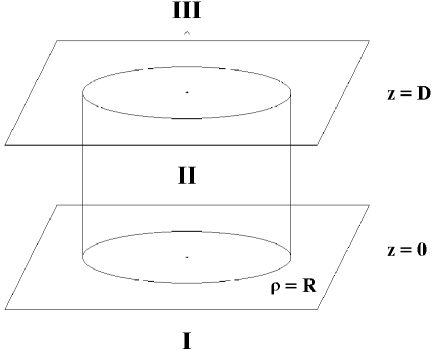
Figure 1: Schematic representation of the situation considered. Region I and Region III are the regions of incidence and transmission. The intermediate Region II contains a cylindrical wire with cosine potentials.

Let us consider two sets of basis states in the boundary regions, namely $\{\Psi_{j}^{\rm I,\pm}\}$ in Region I and $\{\Psi_{j}^{\rm III,\pm}\}$ in Region III. These states are used to expand the wave function in Region I and Region III, for a given value of the energy $E$. The subscript $j$ enumerates the allowed values of $\left\{k_{\rho},m\right\}$ in cylindrical coordinates or $\left\{k_{\rm x},k_{\rm y}\right\}$ in cartesian coordinates, considering applicable boundary conditions and the energy $E$. The $\pm$ signs refer to the propagation direction relative to the $z$ axis, which is oriented from Region I to Region III (see Fig. 1).

We assume our boundary states to be separable in the following way:

$$\Psi_{j}^{\rm I,\pm}(\rho,\phi,z) = \psi_{j}(\rho,\phi)\exp(\pm ik_{z,j}z),$$ (1)

$$\Psi_{j}^{\rm III,\pm}(\rho,\phi,z) = \psi_{j}(\rho,\phi)\exp(\pm ik_{z,j}z),$$ (2)

where $\psi_{j}(\rho,\phi)$ refers to analytical basis functions that account for the $(\rho,\phi)$-dependence of the wave functions (see Sec. III for specific expressions in cylindrical coordinates). These relations will be used to derive band structures from transfer-matrix calculations; they are actually only required for this specific application.

We will describe in this section how scattering solutions that correspond to single incident states $\Psi_{j}^{\rm I,+}$ in Region I or $\Psi_{j}^{\rm III,-}$ in Region III can be derived. We will describe shortly the layer-addition algorithm and finally explain how the band structure associated with the infinite repetition of a basic unit can be extracted from these solutions.

II.1 Basic formulation of the transfer-matrix technique

The first step of the technique consists in establishing solutions associated with single outgoing states $\Psi_{j}^{\rm III,+}$ or incoming states $\Psi_{j}^{\rm III,-}$ in Region III. Since the wave function and its derivatives are entirely defined in Region III, one can propagate these states numerically from $z=D$ to $z=0$, where the solutions are expanded in terms of incident states $\Psi_{j}^{\rm I,+}$ and reflected states $\Psi_{j}^{\rm I,-}$. The numerical techniques that enable the propagation of the wave functions through Region II can be found in Refs 19, 22 and 25. The expansion coefficients of these solutions are stored in ${\bf T}^{\pm\pm}$ matrices and we end up with the following set of solutions:

$$\overline{\Psi}^{+}_{j} \stackrel{{\scriptstyle z\leq 0}}{{=}} \sum_{i}T_{i,j}^{++}\Psi^{\rm I,+}_{i}+\sum_{i}T_{i,j}^{-+}\Psi^{\rm I,-}_{i}\stackrel{{\scriptstyle z\geq D}}{{=}}\Psi^{\rm III,+}_{j},$$ (3)

$$\overline{\Psi}^{-}_{j} \stackrel{{\scriptstyle z\leq 0}}{{=}} \sum_{i}T_{i,j}^{+-}\Psi^{\rm I,+}_{i}+\sum_{i}T_{i,j}^{--}\Psi^{\rm I,-}_{i}\stackrel{{\scriptstyle z\geq D}}{{=}}\Psi^{\rm III,-}_{j}.$$ (4)

In the second step of the procedure, these solutions are combined linearly in order to derive new solutions satisfying the scattering boundary conditions, namely solutions associated with either a single incident state $\Psi_{j}^{\rm I,+}$ in Region I or a single incident state $\Psi_{j}^{\rm III,-}$ in Region III (with this time reflected states in the region of incidence and transmitted states in the other region). Formally, these solutions are expressed in terms of scattering ${\bf S}^{\pm\pm}$ matrices in the following way:

$$\Psi^{+}_{j} \stackrel{{\scriptstyle z\leq 0}}{{=}} \Psi^{\rm I,+}_{j}+\sum_{i}S^{-+}_{i,j}\Psi^{\rm I,-}_{i}\stackrel{{\scriptstyle z\geq D}}{{=}}\sum_{i}S^{++}_{i,j}\Psi^{\rm III,+}_{i},$$ (5)

$$\Psi^{-}_{j} \stackrel{{\scriptstyle z\leq 0}}{{=}} \sum_{i}S^{--}_{i,j}\Psi^{\rm I,-}_{i}\stackrel{{\scriptstyle z\geq D}}{{=}}\Psi_{j}^{\rm III,-}+\sum_{i}S^{+-}_{i,j}\Psi^{\rm III,+}_{i}.$$ (6)

The ${\bf S}^{\pm\pm}$ matrices, which contain the expansion coefficients of these scattering solutions are related to the ${\bf T}^{\pm\pm}$ matrices of Eqs 3 and 4 by ${\bf S}^{++}={{\bf T}^{++}}^{-1}$, ${\bf S}^{-+}={\bf T}^{-+}{{\bf T}^{++}}^{-1}$, ${\bf S}^{--}={\bf T}^{--}-{\bf T}^{-+}{{\bf T}^{++}}^{-1}{\bf T}^{+-}$ and ${\bf S}^{+-}=-{{\bf T}^{++}}^{-1}{\bf T}^{+-}$.

II.2 The layer-addition algorithm for the control of accuracy and the description of periodic systems

To control the numerical instabilities that appear with large distances $D$ (when inverting ${\bf T}^{++}$ to obtain the ${\bf S}^{\pm\pm}$ matrices) or to treat efficiently periodic systems, it is useful to use the layer-addition algorithm.Pendry1 ; Pendry2 Given a subdivision $0=z_{0}<z_{1}<z_{2}<\cdots<z_{n-1}<z_{n}=D$ of the interval $[0,D]$ and referring by ${\bf S}^{++}_{z_{i},z_{j}}$, ${\bf S}^{-+}_{z_{i},z_{j}}$, ${\bf S}^{--}_{z_{i},z_{j}}$ and ${\bf S}^{+-}_{z_{i},z_{j}}$ to the $S$ matrices associated with the interval $[z_{i},z_{j}]$, one can derive those associated with the entire interval $[0,D]$ from the recursive application of the following relations:

$${\bf S}^{++}_{z_{0},z_{i}} = {\bf S}^{++}_{z_{i-1},z_{i}}\left[{\bf I}-{\bf S}^{+-}_{z_{0},z_{i-1}}{\bf S}^{-+}_{z_{i-1},z_{i}}\right]^{-1}{\bf S}^{++}_{z_{0},z_{i-1}},$$ (7)

$${\bf S}^{--}_{z_{0},z_{i}} = {\bf S}^{--}_{z_{0},z_{i-1}}\left[{\bf I}-{\bf S}^{-+}_{z_{i-1},z_{i}}{\bf S}^{+-}_{z_{0},z_{i-1}}\right]^{-1}{\bf S}^{--}_{z_{i-1},z_{i}},$$ (8)

$${\bf S}^{-+}_{z_{0},z_{i}} = {\bf S}^{-+}_{z_{0},z_{i-1}}+{\bf S}^{--}_{z_{0},z_{i-1}}{\bf S}^{-+}_{z_{i-1},z_{i}}\left[{\bf I}-{\bf S}^{+-}_{z_{0},z_{i-1}}{\bf S}^{-+}_{z_{i-1},z_{i}}\right]^{-1}{\bf S}^{++}_{z_{0},z_{i-1}},$$ (9)

$${\bf S}^{+-}_{z_{0},z_{i}} = {\bf S}^{+-}_{z_{i-1},z_{i}}+{\bf S}^{++}_{z_{i-1},z_{i}}{\bf S}^{+-}_{z_{0},z_{i-1}}\left[{\bf I}-{\bf S}^{-+}_{z_{i-1},z_{i}}{\bf S}^{+-}_{z_{0},z_{i-1}}\right]^{-1}{\bf S}^{--}_{z_{i-1},z_{i}}.$$ (10)

These relations enable a straightforward derivation of the ${\bf S}^{\pm\pm}$ matrices associated with the periodic repetition of an arbitrarily large number of units once the transmission through a single unit has been established. Even in the case of non-periodic systems, it is generally useful to use this algorithm since the relative error on the transfer-matrix calculations increases exponentially with the distance $D$ if it is considered in a single step. The number of subdivisions to consider in order to achieve a given accuracy is given, with other considerations on the stability of transfer-matrix calculations, in Ref. 15.

For the derivation of band structures in the next subsection, we will use the ${\bf T}^{\pm\pm}$ matrices. These matrices keep stable when considering large distances $D$ (only the inversion of ${\bf T}^{++}$ is unstable when $D$ is too large). When these matrices are obtained for subdivisions of the $[0,D]$ interval, they can be updated according to the following formula:

$$\begin{pmatrix}{\bf T}^{++}_{z_{0},z_{i}}&{\bf T}^{+-}_{z_{0},z_{i}}\cr{\bf T}^{-+}_{z_{0},z_{i}}&{\bf T}^{--}_{z_{0},z_{i}}\cr\end{pmatrix}=\begin{pmatrix}{\bf T}^{++}_{z_{0},z_{i-1}}&{\bf T}^{+-}_{z_{0},z_{i-1}}\cr{\bf T}^{-+}_{z_{0},z_{i-1}}&{\bf T}^{--}_{z_{0},z_{i-1}}\cr\end{pmatrix}\begin{pmatrix}{\bf T}^{++}_{z_{i-1},z_{i}}&{\bf T}^{+-}_{z_{i-1},z_{i}}\cr{\bf T}^{-+}_{z_{i-1},z_{i}}&{\bf T}^{--}_{z_{i-1},z_{i}}\cr\end{pmatrix}.$$ (11)

II.3 Derivation of band structures from transfer matrices

Let us now consider a basic unit, of length $a$ in the $z$ direction. One can compute the transfer matrices associated with this structure, for given values of the energy $E$. Our objective is to extract from these matrices the band structure characterizing the infinite, periodic repetition of this unit.

For this purpose let us first reconsider the solutions of Eqs 3 and 4, which are recast in the following way:

$$(\overline{\Psi}_{j}^{+}\ldots\overline{\Psi}_{j}^{-})\stackrel{{\scriptstyle z\leq 0}}{{=}}(\Psi_{j}^{\rm I,+}\ldots\Psi_{j}^{\rm I,-})\begin{pmatrix}{\bf T}^{++}&{\bf T}^{+-}\cr{\bf T}^{-+}&{\bf T}^{--}\cr\end{pmatrix}\stackrel{{\scriptstyle z\geq a}}{{=}}(\Psi_{j}^{\rm III,+}\ldots\Psi_{j}^{\rm III,-}).$$ (12)

We want to find combinations $(\overline{\Psi}_{j}^{+}\ldots\overline{\Psi}_{j}^{-}){\bf x}$ of these solutions that satisfy the relation:

$$(\overline{\Psi}_{j}^{+}\ldots\overline{\Psi}_{j}^{-}){\bf x}|_{z=a}=e^{ik_{z}a}\ (\overline{\Psi}_{j}^{+}\ldots\overline{\Psi}_{j}^{-}){\bf x}|_{z=0},$$ (13)

where ${\bf x}$ is a vector that contains the coefficients of these combinations. These combinations describe particular states that keep unchanged after propagation through one period of the system except for a phase factor $\lambda=\exp(ik_{z}a)$. These states are therefore Bloch states associated with a wave vector $k_{z}$ in the first Brillouin zone $[-\pi/a,\pi/a]$ of the periodic system, for the energy $E$ considered. The couples of all possible points $(k_{z},E)$ will represent the band structure of the system.

In order to establish a matricial equation for the calculation of a complete set of Bloch-state solutions, we will write Eq. 13 like

$$(\overline{\Psi}_{j}^{+}\ldots\overline{\Psi}_{j}^{-}){\bf X}|_{z=a}=(\overline{\Psi}_{j}^{+}\ldots\overline{\Psi}_{j}^{-}){\bf X}|_{z=0}\ {\bf\Lambda},$$ (14)

where ${\bf\Lambda}$ is a diagonal matrix containing elements of the form $\lambda=\exp(ik_{z}a)$ and ${\bf X}$ is a matrix whose columns contain the coefficients ${\bf x}$ of each Bloch-state solution.

We have from Eq. 12 that

$$(\overline{\Psi}_{j}^{+}\ldots\overline{\Psi}_{j}^{-}){\bf X}|_{z=a} = (\Psi_{j}^{\rm III,+}\ldots\Psi_{j}^{\rm III,-})|_{z=a}\ {\bf X},$$ (15)

$$(\overline{\Psi}_{j}^{+}\ldots\overline{\Psi}_{j}^{-}){\bf X}|_{z=0} = (\Psi_{j}^{\rm I,+}\ldots\Psi_{j}^{\rm I,-})|_{z=0}\ \begin{pmatrix}{\bf T}^{++}&{\bf T}^{+-}\cr{\bf T}^{-+}&{\bf T}^{--}\cr\end{pmatrix}\ {\bf X}.$$ (16)

If we remember the expression of the basis states $\Psi_{j}^{\rm I,\pm}$ and $\Psi_{j}^{\rm III,\pm}$ (see Eqs 1 and 2), we can actually relate them by

$$(\Psi_{j}^{\rm I,+}\ldots\Psi_{j}^{\rm I,-})|_{z=0}=(\Psi_{j}^{\rm III,+}\ldots\Psi_{j}^{\rm III,-})|_{z=a}\ {\bf diag}[e^{-ik_{z,j}a},\ldots,e^{ik_{z,j}a}],$$ (17)

where ${\bf diag}[]$ stands for a diagonal matrix containing the elements in brackets.

By accounting for Eqs 15, 16 and 17 in Eq. 14, we obtain

$${\bf X}={\bf diag}[e^{-ik_{z,j}a},\ldots,e^{ik_{z,j}a}]\begin{pmatrix}{\bf T}^{++}&{\bf T}^{+-}\cr{\bf T}^{-+}&{\bf T}^{--}\cr\end{pmatrix}{\bf X}\ {\bf\Lambda}$$ (18)

or equivalently

$${\bf X}{\bf\Lambda}^{-1}{\bf X}^{-1}={\bf diag}[e^{-ik_{z,j}a},\ldots,e^{ik_{z,j}a}]\begin{pmatrix}{\bf T}^{++}&{\bf T}^{+-}\cr{\bf T}^{-+}&{\bf T}^{--}\cr\end{pmatrix}.$$ (19)

Eq. 19 implies that the eigenvalues ${\overline{\lambda}}$ of the matrix on the right-hand side of this expression will provide the wave vectors $k_{z}$ that characterize Bloch states associated with the energy $E$ [through $\lambda={\overline{\lambda}}^{-1}=\exp(ik_{z}a)$]. Note that in most techniques the values of $E$ are obtained as a function of $k_{z}$ and that the restriction of $k_{z}$ in the first Brillouin zone $[-\pi/a,\pi/a]$ of the periodic system is automatically verified.

It has to be noted that the values of $\lambda={\overline{\lambda}}^{-1}$ are not always in the form $\exp(ik_{z}a)$, especially in situations involving tunneling processes or in band-gap regions. Many if not all of them can indeed exhibit an exponential dependence $\exp(Ka)$ and are therefore not relevant to the band structure. One distinguishes the values $\lambda$ to consider for the representation of the band structure by the condition $|\lambda|=1$ (within numerical precision).

A numerically more stable technique was formulated by Pendry in Ref. 1 and used by Mayer in Ref. 32 to compute the band structure of carbon nanotubes. It consists in solving the generalized eigenvalue problem

$$\begin{pmatrix}{\bf S}^{++}&0\cr-{\bf S}^{-+}&{\bf I}\cr\end{pmatrix}{\bf x}=\lambda\begin{pmatrix}{\bf I}&-{\bf S}^{+-}\cr 0&{\bf S}^{--}\cr\end{pmatrix}{\bf diag}[e^{-ik_{z,j}a},\ldots,e^{ik_{z,j}a}]\ {\bf x},$$ (20)

where $\lambda$ and ${\bf x}$ are here generalized eigenvalues and eigenvectors (see Appendix A for a demonstration). The $\lambda$ values that are relevant to the band structure are again those that satisfy $|\lambda|=1$ (within numerical precision). They define individual points $(k_{z},E)$ of the band structure through $\lambda=e^{ik_{z}a}$. The restriction of $k_{z}$ in the first Brillouin zone $[-\pi/a,\pi/a]$ of the periodic system is again automatically verified.

For a given problem, these techniques provide a particular representation of the band structure, since its structure in the three-dimensional reciprocal space is projected on the $k_{z}$ axis. This is a consequence of formulating the three-dimensional scattering of the wave function as the one-dimensional propagation of its components. In general this representation is appropriate in situations where a treatment by transfer matrices is relevant.

III Application: band structure and transport properties of cylindrical wires

The applications considered in this paper will focus on the scattering of electrons subject to cosine potentials in a cylindrical wire. We will compute the transmission through a finite number of periods and compare these results with the band structure that characterizes the infinite medium. We will also study the impact of bound states in the intermediate region and discuss the necessity to consider them or not in a transfer-matrix calculation.

We assume that the radius $R$ of the wires is identical to the period $a$ in the $z$ direction. Using cylindrical coordinates, the boundary states we use for the representation of the wave function in Region I and Region III are given by:

$$\Psi_{m,j}^{\rm I/III,\pm}(\rho,\phi,z) = \frac{RJ_{m}(k_{m,j}\rho)\exp(im\phi)}{\sqrt{2\int_{0}^{R}d\rho\rho[J_{m}(k_{m,j}\rho)]^{2}}}\exp(\pm i\sqrt{\frac{2m}{\hbar^{2}}E-k_{m,j}^{2}}z).$$ (21)

The radial wave vectors $k_{m,j}$ that characterizes these states are solutions of $J_{m}^{\prime}(k_{m,j}R)=0$. This condition of vanishing radial derivative of the wave function on the border of the cylinder is imposed in the entire system (Region II included). It enables the wire to allow for at least one solution, namely $k_{0,0}$=0, for any value of the energy $E$. The way the electronic states are propagated through Region II is explained with details in Refs 19, 20, 22 and 25. In order to improve the clarity of the results, only axially symmetric states will be considered.

III.1 Transmission and band structure for a $V(z)=V_{0}\cos(\frac{2\pi}{a}z)$ potential

The first potential we consider is given by $V(z)=V_{0}\cos(\frac{2\pi}{a}z)$, with $V_{0}$= 0.4 eV and $a$=0.434 nm. These parameters are chosen so that a 0.4 eV-wide band gap appears at an electron energy of $\frac{\hbar^{2}}{2m}(\frac{\pi}{a})^{2}$ = 2 eV. After calculation of the transfer matrices associated with a single period $a$ of the potential and using the layer-addition algorithm presented in Sec. II.2, it is straightforward to compute how the electronic transmission in the wire changes as the number of periods increases.

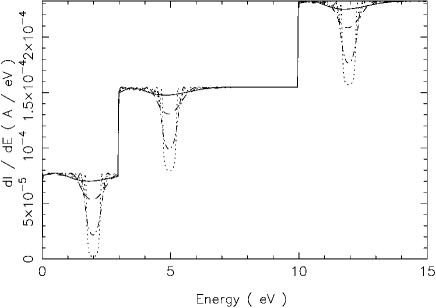
Figure 2: Values of $dI/dE$ after 2 (solid), 4 (dotted), 8 (dot-dashed) and 16 (dotted) periods of a $V(z)=0.4\cos(\frac{2\pi}{a}z)$ eV potential in a cylinder with radius $a$=0.434 nm.

We illustrated in Fig. 2 the electronic transmission (more precisely the values of $dI/dE$) for tube lengths corresponding to 2, 4, 8 and 16 periods of the potential and electron energies ranging from 0 to 15 eV. One can observe the apparition of gaps, which tend to be more pronounced as the number of periods increases. Besides the gaps, the transmission tends to its maximal value and exhibits oscillations that are related to stationary waves in the structure. Indeed their number and the sharpness of their contribution in the transmission diagram increase with the number of periods. Similar observations were made when studying the conduction and field-emission properties of the semiconducting (10,0) carbon nanotube.Mayer27

These non-zero values of the transmission at energies where a band-gap exists when the medium is infinite is due to the finite length of the structures considered here and to the existence of exponentially decaying solutions in these regions. It is only in truly infinite structures that these solutions are prohibited because of their exploding behavior at either $z=+\infty$ or $-\infty$. The existence of decaying solutions in band-gaps was invoked in Ref. 27 to justify the presence of photon-excited electrons in the gap of a nanometer-size (10,0) carbon nanotube in a context of field emission.

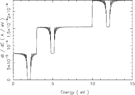
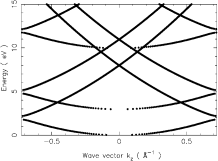
Figure 3: Top: values of $dI/dE$ after 32 periods of a $V(z)=0.4\cos(\frac{2\pi}{a}z)$ eV potential in a cylinder with radius $a$=0.434 nm. Bottom: band structure characterizing the infinite medium.

The values of the transmission after 32 periods of the potential and the band structure characterizing the infinite medium are represented in Fig. 3. The gaps in the transmission diagram are now well pronounced and in agreement with those in the band structure. There is a step in the transmission each time the energy is sufficient to allow for a new state in the radial direction. The occurrence of these steps coincide with the beginning of new bands in the band structure. The height of the steps is given by $2e^{2}/h$ (7.74$\times$10${}^{-5}\Omega^{-1}$), which is twice the value of the conductance quantum since each basis state is representative of two electrons with opposite spins. Because of the value of the period $a$, the gaps follow always by 2 eV the steps in the transmission diagram, which reflects the fact that the band-gaps are always 2 eV higher in energy than the beginning of the new bands.

It is interesting to notice that the energy where all transitions or gaps appear are close to integer values in eV ! In particular, the steps associated with new solutions appear at 3 and 10 eV. This peculiarity can be explained by the fact that the solutions of the boundary condition $J_{0}^{\prime}(k_{0,j}a)=0$ are given in a first approximation by $k_{0,j}a=(j+1/4)\pi$.Abramowitz1 If we remember that $a$ was chosen so that $\frac{\hbar^{2}}{2m}(\frac{\pi}{a})^{2}$ = 2 eV, it can easily be shown that the energy associated with the lateral wave vectors $k_{0,j}$ is given approximately by $E_{0,j}=(2j^{2}+j+1/8)$ eV, which explains our observations and predicts the position of the next steps.

III.2 The issue of bound states with a $V(\rho)=V_{0}\cos(\frac{2\pi}{T}\rho)$ potential

We will now address the issue of bound states in the intermediate Region II and the related question of the number of basis states to consider in this region when doing a transfer-matrix calculation. In the boundary Region I and Region III, the number of basis states is fixed by the condition ${\hbar^{2}k_{m,j}^{2}}/{2m}\leq E$. Indeed basis states with higher $k_{m,j}$ values would be real exponentials in the $z$ direction, carrying no current and causing only instabilities (we assume the potential energy to be zero in Region I and Region III). Since however the potential energy in the intermediate Region II can take negative values, the condition on $k_{m,j}$ inside Region II must be relaxed to ${\hbar^{2}k_{m,j}^{2}}/{2m}\leq E+\Delta E$ and there is the possibility for this region to accommodate additional states, which are exponentially decreasing outside this region but not inside.

This raises an issue on the necessity to consider these bound states or not when doing a transfer-matrix calculation. A first technical difficulty arises from the fact the number of states in Region II is different from that in Region I and Region III. Because of that, connecting the solutions at $z=0$ and $z=D$ involves the inversion of non-square matrices.note All techniques required to deal efficiently with this point were however developed in Ref. 16. Another point is that, according to the literature and for different formulations of the transfer-matrix methodology,Bayman1 ; Wu1 these bound states are likely to cause numerical instabilities. Our objective was therefore to create artificially bound states in our system and study their effect as well as the necessity to consider them or not.

Let us first consider a $V(\rho)=V_{0}\cos(\frac{2\pi}{T}\rho)$ potential, with $V_{0}$=1 eV. The length $D$ and radius $R=2T$ of the cylinder are increased to 1 nm. Because of its $\rho$-dependence - and unlike the previous case - this potential introduces a coupling between the basis states in Region II, which is a necessary condition to observe any effect associated with bound states. Since the potential is independent of $z$, its effect is actually to redefine the electronic states that propagate independently in the wire from the original ones (i.e., states characterized by given values of $m$ and $j$) to combinations of them and one can already understand the necessity to a have enough basis states to represent these new states correctly.

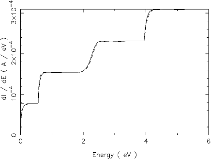
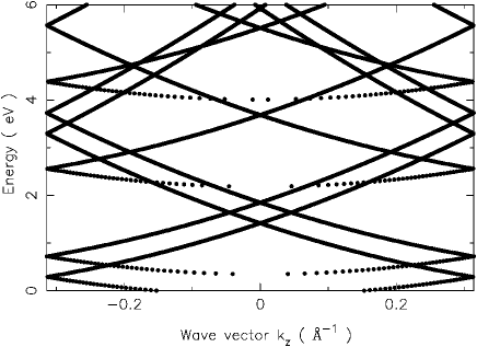
Figure 4: Top: values of $dI/dE$ after $D$=1 nm of a $V(\rho)=\cos(\frac{2\pi}{T}\rho)$ eV potential in a cylinder with radius $R=2T$=1 nm. The solid curve corresponds to $\Delta E$ = 20 eV and the dashed one to $\Delta E$ = 0. Bottom: band structure characterizing the infinite repetition of Region II.

We represented in Fig. 4 the values of $dI/dE$ obtained at $z=D$ as well as the band structure characterizing the infinite repetition of Region II. These results were obtained by considering $\Delta E$=20 eV, i.e. nine basis states within Region II while there are only four of them in Region I and Region III. These additional states serve essentially to remove unphysical discontinuities in the band structure, which appear when the degree of completeness of the basis is poor. The role of $\Delta E$ is identical to the ”cut-off energy” in plane-waves calculations and there is no effect associated with bound states, which are not present here. We checked that these results keep unchanged when considering higher values of $\Delta E$ (up to 50 eV). For the purpose of comparison we represented the values of $dI/dE$ obtained with $\Delta E$=0 (showing that the currents are less sensitive to the completeness of the basis than the band structures).

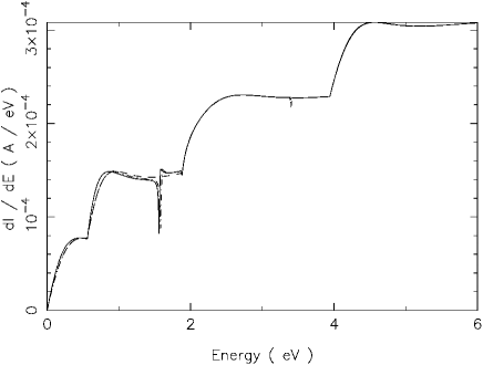
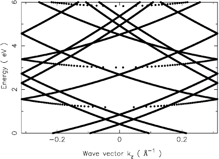
Figure 5: Top: values of $dI/dE$ after $D$=1 nm of a $V(\rho)=\cos(\frac{2\pi}{T}\rho)$-1 eV potential in a cylinder with radius $R=2T$=1 nm. The solid curve corresponds to $\Delta E$ = 20 eV, the dashed one to $\Delta E$ = 0 and the dot-dashed one to $\Delta E$=1 eV. Bottom: band structure characterizing the infinite repetition of Region II.

Let us now consider the $V(\rho)=V_{0}\cos(\frac{2\pi}{T}\rho)-1$ eV potential. We represented in Fig. 5 the corresponding values of $dI/dE$ as well as the band structure that would characterize Region II if repeated periodically. As expected, the band structure is shifted down by 1 eV. This means that the two bands that stood between 0 and 1 eV in Fig. 4 now give rise to discrete energy levels, characterizing bound states. The position of these energy levels is given by the intersection of the former bands with the limits $\pm\pi/D$ of the first Brillouin zone (namely at -0.71 and -0.28 eV), since the length $D$ of Region II is then an integer multiple of half the electronic wave length in the $z$ direction. For the same reason, quasi-bound states in the continuum part of the spectrum ($E\geq 0$) will exist each time the bands of Fig. 5 meet the limits $\pm\pi/D$ of the first Brillouin zone.

Despite the fact these bound states only exist in Region II, they have an impact on the propagative solutions in the $E\geq 0$ range. As observed in previous work,Bayman1 ; Price2 ; Price3 ; Price1 this impact is essentially limited to localized resonances in the $dI/dE$ values, at energies where the interaction between propagative states and (quasi-)bound states is stronger. Indeed the two resonances in Fig. 5 appear at energies where bands meet the border of the first Brillouin zone for the first time (the electronic wave length in the $z$ direction is then identical to that of the bound states, which enhances the interactions).

The results presented here were obtained by taking $\Delta E$ = 20 eV, as required for the completeness of the basis. In particular it is necessary to consider the two bound states (which are part of the solution within Region II). Neglecting them by taking $\Delta E$=0 has indeed a strong impact on both the band structure (all bands are truncated at their beginning on the first eV) and the $dI/dE$ values (the resonances disappear). As illustrated in Fig. 5, taking $\Delta E$ = 1 eV is sufficient to include the bound states and therefore reproduce the resonances and complete the bands. The additional states introduced by taking higher values of $\Delta E$ only improve the completeness of the basis and serve essentially to remove unphysical discontinuities in the bands.

The relation between resonances in the transmission currents and quasi-bound states in the system was well described by Price,Price2 ; Price3 ; Price1 who actually relates them to poles of the $S$ matrix (whose elements are considered as functions of the energy). The present simulations show that these effects are addressed properly, provided additional basis states are considered in the intermediate Region II (through $\Delta E>0$). The ”interior states” do not need to be computed explicitly, nor treated differently from ”open states”.Bayman1 ; Wu1 The specificity of our approach is to use non-square transfer matricesMayer9 to prevent instabilities when making the connection between the different regions.

IV Conclusions

This paper was a pedagogical presentation of the transfer-matrix technique, with an extension to extract the band structure of periodic materials from the $T$ or $S$ matrices associated with a single unit. Because of the transfer-matrix formulation of the scattering problem, the band structure is projected on the $k_{z}$ axis, which is often appropriate in situations where this technique can be applied.

We provided calculations of the transmission and band structure of electrons confined in a cylindrical wire and subject to cosine potentials. We observed how fast the transmission diagram exhibits characteristics predicted by the band structure (namely gaps and steps associated with the opening of new bands), while keeping features associated with their finite length. Comparisons could be made with results obtained for a semiconducting (10,0) carbon nanotube, confirming and providing an insight on processes observed in complex structures.

The issue of bound states was considered. Although they exist only in the intermediate region, they need to be included in the representation because of their impact on propagative solutions (as localized resonances in the transmission) and to avoid unphysical truncations of the band structure. Considering additional states essentially improves the completeness of the representation and removes discontinuities in the bands. The connection between the intermediate region (which may contain ”interior states”) and the boundary regions (which contain only propagative states) is achieved using non-square transfer matrices, making the technique perfectly stable.

Appendix A Derivation of band structures from the ${\bf S}^{\pm\pm}$ matrices

An alternative method for extracting a band structure from the ${\bf S}^{\pm\pm}$ matrices that characterize the basic unit of a periodic system was derived by Pendry.Pendry1 This method is adapted in this Appendix to our formulation of the transfer-matrix technique.

The idea consists in considering the infinite, periodic repetition of a basic unit of length $a$. We will consider that the interfaces between adjacent units are situated at $z=n.a$, with $n$ an integer.

A wave function $\Psi$ can be developed at these interfaces as

$$\Psi(z=n.a)=\sum_{j}c^{+}_{j}[n]\ \Psi^{+}_{j}(z=n.a)+\sum_{j}c^{-}_{j}[n]\ \Psi^{-}_{j}(z=n.a),$$ (22)

where $\Psi^{\pm}_{j}(z=n.a)$ refers to the basis states used at $z=n.a$ for the expansion of the wave function. $c^{\pm}_{j}[n]$ refers to the coefficients of this expansion at $z=n.a$.

From the physical interpretation of the ${\bf S}^{\pm\pm}$ matrices that describe the basic unit cell in the interval $z\in[0,a]$, we can write that

$${\bf c}^{+}[1] = {\bf S}^{++}\ {\bf c}^{+}[0]+{\bf S}^{+-}\ {\bf c}^{-}[1],$$ (23)

$${\bf c}^{-}[0] = {\bf S}^{-+}\ {\bf c}^{+}[0]+{\bf S}^{--}\ {\bf c}^{-}[1],$$ (24)

where ${\bf c}^{\pm}$ refers to vectors that contain the coefficients $c_{j}^{\pm}$. We can reorganize these relations and write them like

$$\begin{pmatrix}{\bf S}^{++}&{\bf 0}\cr-{\bf S}^{-+}&{\bf I}\cr\end{pmatrix}\begin{pmatrix}{\bf c}^{+}[0]\cr{\bf c}^{-}[0]\cr\end{pmatrix}=\begin{pmatrix}{\bf I}&-{\bf S}^{+-}\cr{\bf 0}&{\bf S}^{--}\cr\end{pmatrix}\begin{pmatrix}{\bf c}^{+}[1]\cr{\bf c}^{-}[1]\cr\end{pmatrix}.$$ (25)

We are looking for Bloch-state solutions that satisfy $\Psi(z=a)=e^{ik_{z}a}\ \Psi(z=0)$.

In the context of this paper, we can write that

$$\Psi(z=0) = \sum_{j}c^{+}_{j}[0]\ \Psi^{{\rm I},+}_{j}(z=0)+\sum_{j}c^{-}_{j}[0]\ \Psi^{{\rm I},-}_{j}(z=0)$$ (26)

$$= (\Psi_{j}^{\rm I,+}\ldots\Psi_{j}^{\rm I,-})|_{z=0}\begin{pmatrix}{\bf c}^{+}[0]\cr{\bf c}^{-}[0]\cr\end{pmatrix}$$

and

$$\Psi(z=a) = \sum_{j}c^{+}_{j}[1]\ \Psi^{{\rm III},+}_{j}(z=a)+\sum_{j}c^{-}_{j}[1]\ \Psi^{{\rm III},-}_{j}(z=a)$$ (27)

$$= (\Psi_{j}^{\rm III,+}\ldots\Psi_{j}^{\rm III,-})|_{z=a}\begin{pmatrix}{\bf c}^{+}[1]\cr{\bf c}^{-}[1]\cr\end{pmatrix}.$$

We have also that

$$(\Psi_{j}^{\rm III,+}\ldots\Psi_{j}^{\rm III,-})|_{z=a}=(\Psi_{j}^{\rm I,+}\ldots\Psi_{j}^{\rm I,-})|_{z=0}\ {\bf diag}[e^{ik_{z,j}a},\ldots,e^{-ik_{z,j}a}].$$ (28)

By using Eqs 25 and 28, we can develop $\Psi(z=a)$ as

$$\Psi(z=a)=(\Psi_{j}^{\rm I,+}\ldots\Psi_{j}^{\rm I,-})|_{z=0}\ {\bf diag}[e^{ik_{z,j}a},\ldots,e^{-ik_{z,j}a}]\begin{pmatrix}{\bf I}&-{\bf S}^{+-}\cr{\bf 0}&{\bf S}^{--}\cr\end{pmatrix}^{-1}\begin{pmatrix}{\bf S}^{++}&{\bf 0}\cr-{\bf S}^{-+}&{\bf I}\cr\end{pmatrix}\begin{pmatrix}{\bf c}^{+}[0]\cr{\bf c}^{-}[0]\cr\end{pmatrix}.$$

By using Eqs. 26 and A in the equation $\Psi(z=a)=e^{ik_{z}a}\ \Psi(z=0)$, we finally obtain that

$${\bf diag}[e^{ik_{z,j}a},\ldots,e^{-ik_{z,j}a}]\begin{pmatrix}{\bf I}&-{\bf S}^{+-}\cr{\bf 0}&{\bf S}^{--}\cr\end{pmatrix}^{-1}\begin{pmatrix}{\bf S}^{++}&{\bf 0}\cr-{\bf S}^{-+}&{\bf I}\cr\end{pmatrix}\begin{pmatrix}{\bf c}^{+}[0]\cr{\bf c}^{-}[0]\cr\end{pmatrix}=e^{ik_{z}a}\ \begin{pmatrix}{\bf c}^{+}[0]\cr{\bf c}^{-}[0]\cr\end{pmatrix}$$ (30)

or equivalently the generalized eigenvalue system

$$\begin{pmatrix}{\bf S}^{++}&{\bf 0}\cr-{\bf S}^{-+}&{\bf I}\cr\end{pmatrix}{\bf x}=\lambda\ \begin{pmatrix}{\bf I}&-{\bf S}^{+-}\cr{\bf 0}&{\bf S}^{--}\cr\end{pmatrix}{\bf diag}[e^{-ik_{z,j}a},\ldots,e^{ik_{z,j}a}]\ {\bf x},$$ (31)

where the generalized eigenvalue $\lambda$ will provide the factor $e^{ik_{z}a}$ and the corresponding eigenvector ${\bf x}$ actually provides the coefficients $c^{\pm}_{j}[0]$ of the Bloch-state solution at $z=0$.

Eq. 31 was used by Mayer in Ref. 32 to compute the band structure of carbon nanotubes. The approach described in this Appendix turns out to be numerically more stable than Eq. 19 of the text, which relies on the ${\bf T}^{\pm\pm}$ matrices.

References

- (1) J.B. Pendry, ”Photonic Band Structures,” J. Mod. Opt. 41, 209–229 (1994).
- (2) J.B. Pendry and A. MacKinnon, ”Calculation of Photon Dispersion Relations,” Phys. Rev. Lett. 69, 2772–2775 (1992).
- (3) J.B. Pendry, ”Calculating Photonic Band Structure,” J. Phys. Condens. Mat. 8, 1085–1108 (1996).
- (4) J.-P. Vigneron, I. Derycke, T. Laloyaux, P. Lambin and A.A. Lucas, ”Computation of Scanning Tunneling Microscope Images of Nanometer-sized Objects Physisorbed on Metal Surfaces,” Scanning Microscopy Supplement 7 261–268 (1993).
- (5) W.D. Sheng and J.B. Xia, ”A Transfer Matrix Approach to Conductance in Quantum Waveguides,” J. Phys. Condens Matt. 8 3635–3645 (1994).
- (6) P.St.J. Russel, T.A. Birks and F.D. Lloyds-Lucas, ”Photonic Bloch Waves and Photonic Band Gaps,” in ”Confined Electrons and Photons: New Physics and Applications” (Plenum Press, New York, 1995) pp 585–633.
- (7) A.J. Ward and J.B. Pendry, ”The theory of SNOM: a novel approach,” J. Mod. Opt. 44 1703–1714 (1997).
- (8) B.F. Bayman and C.J. Mehoke, ”Quasibound‐state resonances for a particle in a two‐dimensional well,” Am. J. Phys. 51 875–883 (1983).
- (9) H. Wu and D.L. Sprung, ”Validity of the transfer-matrix method for a two-dimensional electron waveguide,” Appl. Phys. A 58 581–587 (1994).
- (10) M.C. Yalabik, ”Electronic Transport Through a Kink in an Electron Waveguide,” IEEE Trans. Electron Dev. 41 1843–1847 (1994).
- (11) E. Anemogiannis, E.N. Glytsis and T.K. Gaylord, ”Quantum reflection pole method for determination of quasibound states in semiconductor heterostructures,” Superlattices Microstruct. 22 481–496 (1997).
- (12) P.J. Price, ”Space charge in nanostructure resonances,” Superlattices Microstruct. 20 253–260 (1996).
- (13) P.J. Price, ”Space‐charge associated with Fano‐type resonances in nanostructures,” J. Appl. Phys. 79 7381–7382 (1996).
- (14) P.J. Price, ”Quasi-bound states and resonances in heterostructures,” Microelectronics Journal 30 925–934 (1999).
- (15) A. Mayer and J.-P. Vigneron, ”Accuracy-control techniques applied to stable transfer-matrix computations,” Phys. Rev. E 59 4659–4666 (1999).
- (16) A. Mayer and J.-P. Vigneron, ”Non-square transfer-matrix technique applied to the simulation of electronic diffraction by a three-dimensional circular aperture,” Phys. Rev. E 61 5953–5960 (2000).
- (17) A. Mayer and J.-P. Vigneron, ”Group theory used to improve the efficiency of transfer-matrix computations,” Phys. Rev. E 60 7533–7540 (1999).
- (18) V.T. Binh, V. Semet and N. Garcia, ”Nanometric observations at low energy by Fresnel projection microscopy: carbon and polymer fibres,” Ultramicroscopy 58 307–317 (1995).
- (19) A. Mayer and J.-P. Vigneron, ”Real-space formulation of the quantum-mechanical elastic diffusion under n-fold axially symmetric forces,” Phys. Rev. B 56 12599–12607 (1997).
- (20) A. Mayer and J.-P. Vigneron, ”Quantum-mechanical theory of field-emission under axially symmetric forces,” J. Phys. Condens. Matt. 10 869–881 (1998).
- (21) A. Mayer and J.-P. Vigneron, ”Transfer matrices combined with Green’s functions for the multiple-scattering simulation of electronic projection imaging,” Phys. Rev. B 60 2875–2882 (1999).
- (22) A. Mayer, ”A comparative study of the electron transmission through one-dimensional barriers relevant to field-emission problems,” J. Phys. Condens. Mat. 22 175007 (2010).
- (23) A. Mayer, ”Numerical testing of the Fowler-Nordheim equation for the electronic field emission from a flat metal and proposition for an improved equation,” J. Vac. Sci. Technol. B 28 758–762 (2010).
- (24) A. Mayer, ”Exact solutions for the field electron emission achieved from a flat metal using the standard Fowler-Nordheim equation with a correction factor that accounts for the electric field, the work function and the Fermi energy of the emitter,” J. Vac. Sci. Technol. B 29 021803 (2011).
- (25) A. Mayer, M.S. Mousa, M.J. Hagmann and R.G. Forbes, ”Numerical testing by a transfer-matrix technique of Simmons’ equation for the local current density in metal-vacuum-metal junctions,” Jordan Journal of Physics 12 63–77 (2019).
- (26) A. Mayer and J.-P. Vigneron, ”Quantum-mechanical simulations of photon-stimulated field emission by transfer matrices and Green’s functions,” Phys. Rev. B 62 16138–16145 (2000).
- (27) A. Mayer, N.M. Miskovsky and P.H. Cutler, ”Photon-stimulated field emission from semiconducting (10,0) and metallic (5,5) carbon nanotubes,” Phys. Rev. B 65 195416 (2002).
- (28) A. Mayer, M.S. Chung, B.L. Weiss, N.M. Miskovsky and P.H. Cutler, ”Three-dimensional analysis of the geometrical rectifying properties of metal-vacuum-metal junctions and extension for energy conversion,” Phys. Rev. B 77 085411 (2008).
- (29) A. Mayer, M.S. Chung, B.L. Weiss, N.M. Miskovsky and P.H. Cutler, ”Three-dimensional analysis of the rectifying properties of geometrically asymmetric metal-vacuum-metal junctions treated as an oscillating barrier,” Phys. Rev. B 78 205404 (2008).
- (30) A. Mayer, M.S. Chung, P.B. Lerner, B.L. Weiss, N.M. Miskovsky and P.H. Cutler, ”Classical and quantum responsivities of geometrically asymmetric metal-vacuum-metal junctions used for the rectification of infrared and optical radiations,” J. Vac. Sci. Technol. B 29 041802 (2011).
- (31) A. Mayer, M.S. Chung, P.B. Lerner, B.L. Weiss, N.M. Miskovsky and P.H. Cutler, ”Analysis of the efficiency with which geometrically asymmetric metal-vacuum-metal junctions can be used for the rectification of infrared and optical radiations,” J. Vac. Sci. Technol. B 30 31802 (2012).
- (32) A. Mayer, ”Band structure and transport properties of carbon nanotubes using a local pseudopotential and a transfer-matrix technique,” Carbon 42 2057–2066 (2004).
- (33) A. Mayer, N.M. Miskovsky and P.H. Cutler, ”Simulations of field emission from a semiconducting (10,0) carbon nanotube,” J. Vac. Sci. Technol. B 20 100–104 (2002).
- (34) M. Abramowitz and I.A. Stegun, ”Handbook of Mathematical Functions” (Dover Publications Inc., New York, 1972).
- (35) Indeed a reference potential of is assumed between adjacent layers to maintain stability, so the calculations within only involve square transfer matrices. It is only when connecting the solutions with those in Region I and Region III, where the reference potential is zero, that non-square transfer matrices are needed.