Performance Assessment of Kron Reduction in the Numerical Analysis of Polyphase Power Systems

Abstract

This paper investigates the impact of Kron reduction on the performance of numerical methods applied to the analysis of unbalanced polyphase power systems. Specifically, this paper focuses on power-flow study, state estimation, and voltage stability assessment. For these applications, the standard Newton-Raphson method, linear weighted-least-squares regression, and homotopy continuation method are used, respectively. The performance of the said numerical methods is assessed in a series of simulations, in which the zero-injection nodes of a test system are successively eliminated through Kron reduction.

I Introduction

Any application in power system analysis, including Power-Flow Study (PFS), State Estimation (SE), and Voltage Stability Assessment (VSA), inherently relies on equivalent circuits of the power system components. Usually, power grids consist of exactly linear components (e.g., lines) or approximately linear components (e.g., transformers), which can be represented by linear equivalent circuits (e.g., by admittance parameters). Other components, such as generators or loads, do have to be represented by nonlinear equivalent circuits (e.g., to account for power control). Thus, the power system model is described by a system of both linear and nonlinear equations, which can be solved using numerical methods.

Evidently, the computational burden of the aforementioned numerical methods scales with the number of unknowns (i.e., phasors of nodal voltages and/or branch currents). Therefore, model reduction techniques are often employed. In particular, Kron reduction (KR) is commonly used [1, 2]. Fundamentally, KR eliminates nodes with zero current injection from the grid, thereby reducing the number of linear equations (i.e., the order of the admittance matrix). Recently, the authors of this paper performed a rigorous analysis of the feasibility of KR for monophase and polyphase power grids [3, 4]. In line with the said analysis, this paper assesses the impact of KR on the performance of state-of-the-art numerical methods applied to the analysis of polyphase power systems. To be more precise, PFS, SE, and VSA are considered.

The rest of the paper is organized as follows. First, a review of the literature is presented (Sec. II), and the system model is described (Sec. III). Then, the utilized numerical methods are discussed (Sec. IV), and their performance is assessed (Sec. V). Finally, the conclusions are drawn (Sec. VI).

II Literature Review

II-A Power-Flow Study

In PFS, the use of positive-sequence equivalent circuits is common [5]. An overview of numerical methods for solving the Power-Flow Equations (PFEs) is provided in [6]. Notably, fixed-point techniques, like the Gauss-Seidel and Newton-Raphson method (GSM/NRM) [7], or the conjugate-gradient and steepest-descent method [8], are popular.

Naturally, PFS can also be performed for equivalent circuits of polyphase power systems [9]. Indeed, the treatment of the polyphase case is similar to the monophase case. For instance, the PFEs can be written in fixed-point form [10], and be solved using the GSM [11] or NRM [12]. Another method [13], which is notably implemented in EMTP-RV, is based on the so-called modified augmented nodal analysis (a.k.a. MANA).

II-B State Estimation

Here, the estimation of the steady state (i.e., phasors of nodal voltages and/or branch currents) is considered.

SE typically uses positive-sequence equivalent circuits, too. A survey of methods is presented in [14]. Notably, nonlinear or linear Weighted-Least-Squares Regression (WLSR) [15, 16, 17] and the Kalman Filter (KF) [18] are popular. These methods have also been applied polyphase power systems [19, 20].

II-C Voltage Stability Assessment

The term voltage stability refers to a variety of phenomena, ranging from the transient to steady-state timescale [21]. Here, steady-state voltage stability, which is related to the solvability of the PFEs, is considered.

Classical VSA also works with positive-sequence equivalent circuits. Continuation Methods (CMs) (e.g., [22, 23, 24]), a.k.a. Continuation Power Flow (CPF), determine a critical operating point by producing a continuum of PFE solutions. The stability margin can be obtained by solving a nonlinear program [25]. Alternatively, the solvability of the PFEs can be assessed using Voltage Stability Indices (VSIs), like the singular values [26], eigenvalues [27], or determinant [28] of the Jacobian matrix. Notably, CPF methods [29] and VSIs [30] have been applied to polyphase power systems.

II-D Contribution of this Paper

This paper investigates the impact of KR on the performance of state-of-the-art numerical methods for PFS, SE, and VSA, which are applied to the analysis of unbalanced polyphase power systems. More precisely, the standard NRM is used for PFS, linear WLSR for SE, and the homotopy CM for VSA.

III System Model

This section is a summary of the models discussed in [4, 30]. Unless stated otherwise, quantities are expressed in per unit.

III-A Electrical Grid

Figure 1: Definition of the compound branch impedance matrices $\boldsymbol{\mathbf{Z}}_{\ell}$ ($\ell\in\mathcal{L}$), compound shunt admittance matrices $\boldsymbol{\mathbf{Y}}_{t}$ ($t\in\mathcal{T}$), nodal phase-to-ground voltage vectors $\boldsymbol{\mathbf{V}}_{n}$, and injected current vectors $\boldsymbol{\mathbf{I}}_{n}$ ($n\in\mathcal{N}$).

Consider a generic polyphase power grid, which is equipped with a neutral conductor. The system is wired as follows:

Hypothesis 1.

The neutral conductor is effectively grounded (i.e., the neutral-to-ground voltage is zero), and it is connected to the reference points of all voltage or current sources.

That is, the phase-to-neutral voltages are effectively referenced w.r.t. the ground, and fully describe the system.

The ground node is denoted by $\mathcal{G}$, and the polyphase nodes, each of which has a complete set of phase terminals $\mathcal{P}$, by $\mathcal{N}$. The equivalent circuit of the grid is composed of polyphase branches $\mathcal{L}\subseteq\mathcal{N}\times\mathcal{N}$ and polyphase shunts $\mathcal{T}=\mathcal{N}\times\mathcal{G}$, which are characterized by compound branch impedance matrices $\boldsymbol{\mathbf{Z}}_{\ell}$ ($\ell\in\mathcal{L}$) and compound shunt admittance matrices $\boldsymbol{\mathbf{Y}}_{t}$ ($t\in\mathcal{T}$), respectively (see Fig. 1). It is supposed that

Hypothesis 2.

The compound electrical parameters satisfy

$$\forall\boldsymbol{\mathbf{Z}}_{\ell} :~{} \boldsymbol{\mathbf{Z}}_{\ell} =\boldsymbol{\mathbf{Z}}_{\ell}^{\top},~{} \exists\boldsymbol{\mathbf{Y}}_{\ell} =\boldsymbol{\mathbf{Z}}_{\ell}^{-1},~{} \Re\left\{\boldsymbol{\mathbf{Z}}_{\ell}\right\} \succeq 0$$ (1)

$$\text{if}~{}\boldsymbol{\mathbf{Y}}_{t}\neq\boldsymbol{\mathbf{0}} :~{} \boldsymbol{\mathbf{Y}}_{t} =\boldsymbol{\mathbf{Y}}_{t}^{\top},~{} \exists\boldsymbol{\mathbf{Z}}_{t} =\boldsymbol{\mathbf{Y}}_{t}^{-1},~{} \Re\left\{\boldsymbol{\mathbf{Y}}_{t}\right\} \succeq 0$$ (2)

The topology is described by the branch graph $\mathfrak{B}\coloneqq(\mathcal{N},\mathcal{L})$ and the shunt graph $\mathfrak{S}\coloneqq(\mathcal{N}\cup\mathcal{G},\mathcal{T})$.

Let $V_{n,p}$ and $I_{n,p}$ the phasors of the phase-to-ground voltage and injected current in phase $p$ of node $n$, respectively. Define corresponding vectors for the nodes (see Fig. 1) and the grid

$$\boldsymbol{\mathbf{V}}_{n} \coloneqq\operatorname{col}_{p\in\mathcal{P}}\left(V_{n,p}\right),~{} \boldsymbol{\mathbf{V}} \coloneqq\operatorname{col}_{n\in\mathcal{N}}\left(\boldsymbol{\mathbf{V}}_{n}\right)$$ (3)

$$\boldsymbol{\mathbf{I}}_{n} \coloneqq\operatorname{col}_{p\in\mathcal{P}}\left(I_{n,p}\right),~{} \boldsymbol{\mathbf{I}} \coloneqq\operatorname{col}_{n\in\mathcal{N}}\left(\boldsymbol{\mathbf{I}}_{n}\right)$$ (4)

Further, let $\boldsymbol{\mathbf{A}}_{\mathfrak{B}}$ be the (edge-to-vertex) incidence matrix of $\mathfrak{B}$. As this matrix is uniquely defined irrespective of the topology, the proposed model applies to both radial and meshed grids. The primitive compound admittance matrices $\boldsymbol{\mathbf{Y}}_{\mathcal{L}}$ and $\boldsymbol{\mathbf{Y}}_{\mathcal{T}}$, and the polyphase incidence matrix $\boldsymbol{\mathbf{A}}_{\mathfrak{B}}^{\mathcal{P}}$ are defined as

$$\boldsymbol{\mathbf{Y}}_{\mathcal{L}} \coloneqq\operatorname{diag}_{\ell\in\mathcal{L}}\left(\boldsymbol{\mathbf{Y}}_{\ell}\right),~{}\boldsymbol{\mathbf{Y}}_{\mathcal{T}}\coloneqq\operatorname{diag}_{t\in\mathcal{T}}\left(\boldsymbol{\mathbf{Y}}_{t}\right)$$ (5)

$$\boldsymbol{\mathbf{A}}_{\mathfrak{B}}^{\mathcal{P}} \coloneqq\boldsymbol{\mathbf{A}}_{\mathfrak{B}}\otimes\operatorname{diag}\left(\boldsymbol{\mathbf{1}}_{\left|\mathcal{P}\right|}\right)$$ (6)

where $\otimes$ is the Kronecker product, and $\boldsymbol{\mathbf{1}}_{\left|\mathcal{P}\right|}$ is a column vector of ones with length $\left|\mathcal{P}\right|$. The compound admittance matrix $\boldsymbol{\mathbf{Y}}$, which establishes the relation $\boldsymbol{\mathbf{I}}=\boldsymbol{\mathbf{Y}}\boldsymbol{\mathbf{V}}$, is given by

$$\boldsymbol{\mathbf{Y}}=(\boldsymbol{\mathbf{A}}_{\mathfrak{B}}^{\mathcal{P}})^{\top}\boldsymbol{\mathbf{Y}}_{\mathcal{L}}\boldsymbol{\mathbf{A}}_{\mathfrak{B}}^{\mathcal{P}}+\boldsymbol{\mathbf{Y}}_{\mathcal{T}}$$ (7)

Accordingly, the injected powers $\boldsymbol{\mathbf{S}}(\boldsymbol{\mathbf{V}})$ are given by

$$\boldsymbol{\mathbf{S}}(\boldsymbol{\mathbf{V}})\coloneqq\boldsymbol{\mathbf{V}}\circ(\boldsymbol{\mathbf{Y}}\boldsymbol{\mathbf{V}})^{*}$$ (8)

where $\circ$ is the Hadamard product and ^∗ the complex conjugate.

Let $\mathcal{A}$ and $\mathcal{B}$ be nonempty disjoint subsets of $\mathcal{N}$. Moreover, let $\boldsymbol{\mathbf{I}}_{\mathcal{A}}$, $\boldsymbol{\mathbf{V}}_{\mathcal{B}}$, and $\boldsymbol{\mathbf{Y}}_{\mathcal{A}\times\mathcal{B}}$ be the associated blocks of $\boldsymbol{\mathbf{I}}$, $\boldsymbol{\mathbf{V}}$, and $\boldsymbol{\mathbf{Y}}$, respectively. It holds that (for proof, see [4]):

Lemma 1 (Kron Reduction).

Let $\mathcal{Z}\subsetneq\mathcal{N},~{}\mathcal{Z}\neq\emptyset$ s.t. $\boldsymbol{\mathbf{I}}_{\mathcal{Z}}=\boldsymbol{\mathbf{0}}$, and $\mathcal{Z}_{\complement}\coloneqq\mathcal{N}\setminus\mathcal{Z}$. If Hyps. 1–2 hold, $\mathfrak{B}$ is weakly connected, and $\Re\{\boldsymbol{\mathbf{Z}}_{\ell}\}\succ 0$ $\forall\ell\in\mathcal{L}$, then $\boldsymbol{\mathbf{V}}_{\mathcal{Z}}$ is a linear function of $\boldsymbol{\mathbf{V}}_{\mathcal{Z}_{\complement}}$

$$\boldsymbol{\mathbf{V}}_{\mathcal{Z}}=-\boldsymbol{\mathbf{Y}}^{-1}_{\mathcal{Z}\times\mathcal{Z}}\boldsymbol{\mathbf{Y}}_{\mathcal{Z}\times\mathcal{Z}_{\complement}}\boldsymbol{\mathbf{V}}_{\mathcal{Z}_{\complement}}$$ (9)

As a result, $\boldsymbol{\mathbf{I}}=\boldsymbol{\mathbf{Y}}\boldsymbol{\mathbf{V}}$ can be reduced to

$$\boldsymbol{\mathbf{I}}_{\mathcal{Z}_{\complement}}=(\boldsymbol{\mathbf{Y}}/\boldsymbol{\mathbf{Y}}_{\mathcal{Z}\times\mathcal{Z}})\boldsymbol{\mathbf{V}}_{\mathcal{Z}_{\complement}}$$ (10)

where $\boldsymbol{\mathbf{Y}}/\boldsymbol{\mathbf{Y}}_{\mathcal{Z}\times\mathcal{Z}}$ is the Schur complement of $\boldsymbol{\mathbf{Y}}$ w.r.t. $\boldsymbol{\mathbf{Y}}_{\mathcal{Z}\times\mathcal{Z}}$.

III-B Aggregate Node Behavior

The nodes $\mathcal{N}$ are divided into slack nodes $\mathcal{S}$, resource nodes $\mathcal{R}$, and zero-injection nodes $\mathcal{Z}$ (i.e., $\mathcal{N}=\mathcal{S}\cup\mathcal{R}\cup\mathcal{Z}$).

Slack nodes are represented by Thévenin Equivalents (TEs). The TE of slack node $s\in\mathcal{S}$ consists of a voltage source $\boldsymbol{\mathbf{V}}_{\text{TE},s}$ and an impedance $\boldsymbol{\mathbf{Z}}_{\text{TE},s}$. Supposing $\exists\boldsymbol{\mathbf{Y}}_{\text{TE},s}\coloneqq\boldsymbol{\mathbf{Z}}_{\text{TE},s}^{-1}$, define

$$\boldsymbol{\mathbf{S}}_{\text{TE},s}(\boldsymbol{\mathbf{V}}_{s}) \coloneqq\boldsymbol{\mathbf{V}}_{s}\circ\left(\boldsymbol{\mathbf{Y}}_{\text{TE},s}(\boldsymbol{\mathbf{V}}_{\text{TE},s}-\boldsymbol{\mathbf{V}}_{s})\right)^{*}$$ (11)

$$\boldsymbol{\mathbf{S}}_{\text{TE}}(\boldsymbol{\mathbf{V}}_{\mathcal{S}}) \coloneqq\operatorname{col}_{s\in\mathcal{S}}(\boldsymbol{\mathbf{S}}_{\text{TE},s}(\boldsymbol{\mathbf{V}}_{s}))$$ (12)

Resource nodes are modeled by Polynomial Models (PMs). The power injected into phase $p\in\mathcal{P}$ of resource node $r\in\mathcal{R}$ is represented by a quadratic polynomial

$$\boldsymbol{\mathbf{S}}_{\text{PM},r,p}(V_{r,p},\lambda_{r,p}) \coloneqq\lambda_{r,p}\left[\begin{aligned} P_{0,r,p}&f_{\Re,r,p}(V_{r,p})\\ +jQ_{0,r,p}&f_{\Im,r,p}(V_{r,p})\end{aligned}\right.$$ (13)

$$f_{\Re,r,p}(V_{r,p}) \coloneqq\alpha_{\Re,r,p}\left|\frac{V_{r,p}}{V_{0,r}}\right|^{2}+\beta_{\Re,r,p}\left|\frac{V_{r,p}}{V_{0,r}}\right|+\gamma_{\Re,r,p}$$ (14)

$$f_{\Im,r,p}(V_{r,p}) \coloneqq\alpha_{\Im,r,p}\left|\frac{V_{r,p}}{V_{0,r}}\right|^{2}+\beta_{\Im,r,p}\left|\frac{V_{r,p}}{V_{0,r}}\right|+\gamma_{\Im,r,p}$$ (15)

where $\lambda$ is a loading factor, $P_{0},Q_{0},V_{0}$ are reference values, and $\alpha,\beta,\gamma$ are normalized coefficients. Furthermore, define

$$\boldsymbol{\mathbf{S}}_{\text{PM},r}(\boldsymbol{\mathbf{V}}_{r},\boldsymbol{\mathbf{\lambda}}_{r}) =\operatorname{col}_{p\in\mathcal{P}}\left(\boldsymbol{\mathbf{S}}_{\text{PM},r}(V_{r,p},\lambda_{r})\right)$$ (16)

$$\boldsymbol{\mathbf{S}}_{\text{PM}}(\boldsymbol{\mathbf{V}}_{\mathcal{R}},\boldsymbol{\mathbf{\lambda}}) =\operatorname{col}_{r\in\mathcal{R}}\left(\boldsymbol{\mathbf{S}}_{\text{PM},r}(\boldsymbol{\mathbf{V}}_{r},\boldsymbol{\mathbf{\lambda}}_{r})\right)$$ (17)

Zero-injection nodes have zero injected current in all phases. By consequence, the injected powers are zero:

$$\mathbf{S}_{\mathcal{Z}}(\boldsymbol{\mathbf{V}})=\mathbf{0}$$ (18)

Finally, note that slack nodes and resource nodes correspond to $V\delta$ buses and $PQ$ buses, respectively. Due to lack of space, PV buses are not considered in this paper, but their treatment is straightforward [31].

IV Numerical Methods

IV-A Power-Flow Study

The combination of (8), (12), (17) and (18) yields the PFEs in the form of mismatch equations. Namely

$$\Delta\boldsymbol{\mathbf{S}}(\boldsymbol{\mathbf{V}},\boldsymbol{\mathbf{\lambda}})\coloneqq\boldsymbol{\mathbf{S}}(\boldsymbol{\mathbf{V}})-\left[\begin{array}[]{l}\boldsymbol{\mathbf{S}}_{\text{TE}}(\boldsymbol{\mathbf{V}}_{\mathcal{S}})\\ \boldsymbol{\mathbf{S}}_{\text{PM}}(\boldsymbol{\mathbf{V}}_{\mathcal{R}},\boldsymbol{\mathbf{\lambda}})\\ \boldsymbol{\mathbf{0}}_{\left|\mathcal{Z}\right|\times 1}\\ \end{array}\right]=\boldsymbol{\mathbf{0}}$$ (19)

Express $\Delta\boldsymbol{\mathbf{S}}(\boldsymbol{\mathbf{V}},\boldsymbol{\mathbf{\lambda}})$ in rectangular and $\boldsymbol{\mathbf{V}}$ in polar coordinates, i.e. $\Delta\boldsymbol{\mathbf{S}}(\boldsymbol{\mathbf{V}},\boldsymbol{\mathbf{\lambda}})\coloneqq\Delta\boldsymbol{\mathbf{P}}(\boldsymbol{\mathbf{V}},\boldsymbol{\mathbf{\lambda}})+j\Delta\boldsymbol{\mathbf{Q}}(\boldsymbol{\mathbf{V}},\boldsymbol{\mathbf{\lambda}})$ and $\boldsymbol{\mathbf{V}}\coloneqq\boldsymbol{\mathbf{E}}\angle\boldsymbol{\mathbf{\theta}}$. For fixed $\boldsymbol{\mathbf{\lambda}}=\boldsymbol{\mathbf{\lambda}}_{\star}$, (19) can be reformulated as

$$\boldsymbol{\mathbf{f}}(\boldsymbol{\mathbf{E}},\boldsymbol{\mathbf{\theta}})\coloneqq\left[\begin{array}[]{l}\Delta\boldsymbol{\mathbf{P}}(\boldsymbol{\mathbf{E}}\angle\boldsymbol{\mathbf{\theta}},\boldsymbol{\mathbf{\lambda}}_{\star})\\ \Delta\boldsymbol{\mathbf{Q}}(\boldsymbol{\mathbf{E}}\angle\boldsymbol{\mathbf{\theta}},\boldsymbol{\mathbf{\lambda}}_{\star})\end{array}\right]=\boldsymbol{\mathbf{0}}$$ (20)

This equation can be solved with the NRM in Alg. 1 (see [12]). Here, $\boldsymbol{\mathbf{x}}_{\text{PFS}}\coloneqq[\boldsymbol{\mathbf{E}};\boldsymbol{\mathbf{\theta}}]$ are the unknowns, $\operatorname{D}_{\boldsymbol{\mathbf{x}}}\boldsymbol{\mathbf{f}}$ is the Jacobian matrix, and $\varepsilon$ the convergence tolerance.

Algorithm 1 NRM for $\boldsymbol{\mathbf{f}}(\boldsymbol{\mathbf{x}})=\boldsymbol{\mathbf{0}}$.

procedure NRM($\boldsymbol{\mathbf{f}}(\boldsymbol{\mathbf{x}})$, $\boldsymbol{\mathbf{x}}_{0}$)$\triangleright$ Initial guess $\boldsymbol{\mathbf{x}}_{0}$.

     for $i\geqslant 0$ do

         $\Delta\boldsymbol{\mathbf{f}}\leftarrow\boldsymbol{\mathbf{f}}(\boldsymbol{\mathbf{x}}_{i})$

         if $\left\lVert\Delta\boldsymbol{\mathbf{f}}\right\rVert\leqslant\varepsilon$ then$\triangleright$ Convergence.

              break

         else$\triangleright$ Correction step.

              $\boldsymbol{\mathbf{J}}\leftarrow\operatorname{D}_{\boldsymbol{\mathbf{x}}}\boldsymbol{\mathbf{f}}(\boldsymbol{\mathbf{x}}_{i})$

              $\Delta\boldsymbol{\mathbf{x}}\leftarrow\text{solve}\left(\boldsymbol{\mathbf{J}}\Delta\boldsymbol{\mathbf{x}}=\Delta\boldsymbol{\mathbf{f}},\Delta\boldsymbol{\mathbf{x}}\right)$

              $\boldsymbol{\mathbf{x}}_{i+1}\leftarrow\boldsymbol{\mathbf{x}}_{i}-\Delta\boldsymbol{\mathbf{x}}$

         end if

     end for

     return $\boldsymbol{\mathbf{x}}_{i}$$\triangleright$ Final solution $\boldsymbol{\mathbf{x}}_{i}$.

end procedure

IV-B State Estimation

The slack and resource nodes are equipped with Phasor Measurement Units (PMUs), and the zero-injection nodes are treated as virtual measurements [32]. Note that $\mathcal{S}\cup\mathcal{R}=\mathcal{Z}_{\complement}$. Let $\widetilde{\boldsymbol{\mathbf{V}}}_{\mathcal{Z}_{\complement}}$ and $\widetilde{\boldsymbol{\mathbf{I}}}_{\mathcal{Z}_{\complement}}$ be the PMU measurements, $\widetilde{\boldsymbol{\mathbf{I}}}_{\mathcal{Z}}\coloneqq\boldsymbol{\mathbf{0}}_{\left|\mathcal{Z}\right|\times 1}$ the virtual ones, and $\widetilde{\boldsymbol{\mathbf{I}}}\coloneqq\operatorname{col}(\widetilde{\boldsymbol{\mathbf{I}}}_{\mathcal{Z}_{\complement}},\widetilde{\boldsymbol{\mathbf{I}}}_{\mathcal{Z}})$. Express the states and measurements in rectangular coordinates

$$\boldsymbol{\mathbf{x}}_{\text{SE}}\coloneqq\left[\begin{array}[]{l}\Re\left\{\boldsymbol{\mathbf{V}}\right\}\\ \Im\left\{\boldsymbol{\mathbf{V}}\right\}\\ \end{array}\right],~{}\boldsymbol{\mathbf{y}}\coloneqq\left[\begin{array}[]{l}\Re\{\widetilde{\boldsymbol{\mathbf{V}}}_{\mathcal{Z}_{\complement}}\}\\ \Im\{\widetilde{\boldsymbol{\mathbf{V}}}_{\mathcal{Z}_{\complement}}\}\\ \Re\{\widetilde{\boldsymbol{\mathbf{I}}}\}\\ \Im\{\widetilde{\boldsymbol{\mathbf{I}}}\}\end{array}\right]$$ (21)

and assume that the measurement noise is white and Gaussian. This yields a linear measurement model [19]

$$\mathbf{y}=\mathbf{C}\mathbf{x}_{\text{SE}}+\mathbf{v},~{}\mathbf{v}\sim\mathbf{N}(\mathbf{0},\mathbf{R})$$ (22)

where $\mathbf{N}(\mathbf{0},\mathbf{R})$ is the multivariate normal distribution with mean vector $\boldsymbol{\mathbf{0}}$ and covariance matrix $\boldsymbol{\mathbf{R}}$. $\boldsymbol{\mathbf{C}}$ is built as follows

$$\boldsymbol{\mathbf{C}}=\left[\begin{array}[]{ll}\boldsymbol{\mathbf{\Gamma}}&\phantom{-}\boldsymbol{\mathbf{0}}\\ \boldsymbol{\mathbf{0}}&\phantom{-}\boldsymbol{\mathbf{\Gamma}}\\ \boldsymbol{\mathbf{G}}&-\boldsymbol{\mathbf{B}}\\ \boldsymbol{\mathbf{B}}&\phantom{-}\boldsymbol{\mathbf{G}}\\ \end{array}\right]$$ (23)

where $\boldsymbol{\mathbf{\Gamma}}$ is the indicator function for the voltages $\boldsymbol{\mathbf{V}}_{Z_{\complement}}$

$$\boldsymbol{\mathbf{\Gamma}}\in\mathbb{R}^{\left|\mathcal{Z}_{\complement}\right|\times\left|\mathcal{N}\right|},~{}\Gamma_{mn}\coloneqq\left\{\begin{array}[]{ll}1&\text{if}~{}m=n\\ 0&\text{otherwise}\end{array}\right.$$ (24)

and $\boldsymbol{\mathbf{G}}\coloneqq\Re\left\{\boldsymbol{\mathbf{Y}}\right\}$, $\boldsymbol{\mathbf{B}}\coloneqq\Im\left\{\boldsymbol{\mathbf{Y}}\right\}$. The linear WLSR in Alg. 2 yields an estimate $\widehat{\boldsymbol{\mathbf{x}}}_{\text{SE}}$ with minimum squared error (see [19]).

Algorithm 2 Linear WLSR for $\boldsymbol{\mathbf{y}}=\boldsymbol{\mathbf{C}}\boldsymbol{\mathbf{x}}+\boldsymbol{\mathbf{v}}$, $\boldsymbol{\mathbf{v}}\sim\boldsymbol{\mathbf{N}}(\boldsymbol{\mathbf{0}},\boldsymbol{\mathbf{R}})$.

procedure LWLSR($\boldsymbol{\mathbf{y}},\boldsymbol{\mathbf{C}},\boldsymbol{\mathbf{R}}$)

     $\boldsymbol{\mathbf{G}}\leftarrow\boldsymbol{\mathbf{C}}^{\top}\boldsymbol{\mathbf{R}}^{-1}\boldsymbol{\mathbf{C}}$$\triangleright$ Gain matrix.

     $\widehat{\boldsymbol{\mathbf{x}}}\leftarrow\boldsymbol{\mathbf{G}}^{-1}\boldsymbol{\mathbf{C}}^{\top}\boldsymbol{\mathbf{R}}^{-1}\boldsymbol{\mathbf{y}}$

     return $\widehat{\boldsymbol{\mathbf{x}}}$

end procedure

IV-C Voltage Stability Assessment

Suppose that $\boldsymbol{\mathbf{\lambda}}$ follows the trajectory $\boldsymbol{\mathbf{\lambda}}(\lambda)\coloneqq\boldsymbol{\mathbf{\lambda}}_{0}+\lambda\cdot\boldsymbol{\mathbf{t}}$ with origin $\boldsymbol{\mathbf{\lambda}}_{0}$ and direction $\boldsymbol{\mathbf{t}}$. Define $\boldsymbol{\mathbf{g}}(\boldsymbol{\mathbf{E}},\boldsymbol{\mathbf{\theta}},\lambda)$ as the analogon of $\boldsymbol{\mathbf{f}}(\boldsymbol{\mathbf{E}},\boldsymbol{\mathbf{\theta}})$, which includes the trajectory $\boldsymbol{\mathbf{\lambda}}(\lambda)$. Namely

$$\boldsymbol{\mathbf{g}}(\boldsymbol{\mathbf{E}},\boldsymbol{\mathbf{\theta}},\lambda)\coloneqq\left[\begin{array}[]{l}\Delta\boldsymbol{\mathbf{P}}(\boldsymbol{\mathbf{E}}\angle\boldsymbol{\mathbf{\theta}},\boldsymbol{\mathbf{\lambda}}(\lambda))\\ \Delta\boldsymbol{\mathbf{Q}}(\boldsymbol{\mathbf{E}}\angle\boldsymbol{\mathbf{\theta}},\boldsymbol{\mathbf{\lambda}}(\lambda))\end{array}\right]=\boldsymbol{\mathbf{0}}$$ (25)

The objective of VSA is to find the maximum $\lambda$ for which the above-stated equations remains solvable. That is

$$\max\lambda~{}\text{s.t.}~{}\boldsymbol{\mathbf{g}}(\boldsymbol{\mathbf{E}},\boldsymbol{\mathbf{\theta}},\lambda)=\boldsymbol{\mathbf{0}}$$ (26)

CPF methods solve this optimization problem by producing a continuum of solutions of (25). For this, the homotopy CM in Alg. 3 is used (see [24, 29]). Note that $\boldsymbol{\mathbf{x}}_{\text{VSA}}\coloneqq[\boldsymbol{\mathbf{E}};\boldsymbol{\mathbf{\theta}}]$, $\xi\coloneqq\lambda$ are the unknowns, and $\sigma$ is the step size used for continuation. The CM employs a predictor to calculate guesses $\boldsymbol{\mathbf{x}}^{-}_{k+1}$, $\xi^{-}_{k+1}$ of the next solutions in the continuum, and a corrector to find the actual values $\boldsymbol{\mathbf{x}}^{+}_{k+1}$, $\xi^{+}_{k+1}$. The predictor is based on the tangent method, and the corrector on the NRM.

Algorithm 3 Homotopy CM for $\max\xi$ s.t. $\boldsymbol{\mathbf{g}}(\boldsymbol{\mathbf{x}},\xi)=\boldsymbol{\mathbf{0}}$.

procedure HCM($\boldsymbol{\mathbf{g}}(\boldsymbol{\mathbf{x}},\xi)$, $\boldsymbol{\mathbf{x}}_{0}$, $\xi_{0}$)$\triangleright$ Starting point $\boldsymbol{\mathbf{x}}_{0},\xi_{0}$.

     for k$\geqslant 0$ do

         # Predictor (tangent method)

         $d\boldsymbol{\mathbf{x}}\leftarrow\text{solve}\left(\operatorname{D}_{\boldsymbol{\mathbf{x}}}\boldsymbol{\mathbf{g}}(\boldsymbol{\mathbf{x}}_{k},\xi_{k})d\boldsymbol{\mathbf{x}}=-\operatorname{D}_{\xi}\boldsymbol{\mathbf{g}}(\boldsymbol{\mathbf{x}}_{k},\xi_{k}),d\boldsymbol{\mathbf{x}}\right)$

         $\left[\begin{array}[]{l}\boldsymbol{\mathbf{x}}^{-}_{k+1}\\ \xi^{-}_{k+1}\end{array}\right]=\left[\begin{array}[]{l}\boldsymbol{\mathbf{x}}_{k}\\ \xi_{k}\end{array}\right]+\sigma\left(\frac{1}{\sqrt{\left\lVert d\boldsymbol{\mathbf{x}}\right\rVert^{2}+1}}\left[\begin{array}[]{c}d\boldsymbol{\mathbf{x}}\\ 1\end{array}\right]\right)$

         # Corrector (NRM)

         $\boldsymbol{\mathbf{h}}([\boldsymbol{\mathbf{x}};\xi])\coloneqq\left[\begin{array}[]{l}\boldsymbol{\mathbf{g}}(\boldsymbol{\mathbf{x}},\xi)\\ \left\lVert\boldsymbol{\mathbf{x}}-\boldsymbol{\mathbf{x}}_{k}\right\rVert^{2}+(\xi-\xi_{k})^{2}-\sigma^{2}\end{array}\right]$

         $[\boldsymbol{\mathbf{x}}^{+}_{k+1};\xi^{+}_{k+1}]\leftarrow\text{NRM}\left(\boldsymbol{\mathbf{h}}([\boldsymbol{\mathbf{x}};\xi]),[\boldsymbol{\mathbf{x}}^{-}_{k+1};\xi^{-}_{k+1}]\right)$

         $\left[\begin{array}[]{l}\boldsymbol{\mathbf{x}}_{k+1}\\ \xi_{k+1}\end{array}\right]\leftarrow\left[\begin{array}[]{l}\boldsymbol{\mathbf{x}}^{+}_{k+1}\\ \xi^{+}_{k+1}\end{array}\right]$

         if $\operatorname{sign}(\xi_{k+1}-\xi_{k})\leqslant 0$ then$\triangleright$ Maximum $\xi$.

              break

         end if

     end for

     return $\{\boldsymbol{\mathbf{x}}_{k},\xi_{k}\}$$\triangleright$ Continuum of solutions $\{\boldsymbol{\mathbf{x}}_{k},\xi_{k}\}$.

end procedure

V Performance Assessment

V-A Test System & Simulation Setup

Figure 2: Single-line diagram of the test system. The nodes comprise one slack node $\mathcal{S}=\{\text{S}\}$, 15 resource nodes $\mathcal{R}=\{\text{G1--G5}\}\cup\{\text{L1--L5}\}\cup\{\text{C1--C5}\}$, and 100 zero-injection nodes $\mathcal{Z}=\{\text{Z1--Z100}\}$. The lines are untransposed, and of type IEEE-300 (black) and IEEE-301 (gray), respectively (see [33]).

The numerical methods discussed in Sec. IV are applied to an unbalanced three-phase power grid. The single-line diagram of the test system is depicted in Fig. 2. The grid is composed of untransposed overhead lines of 5 km length each, which are configured according to the codes IEEE-300 and IEEE-301 from [33]. The system has 1 slack node (S), 15 resource nodes (i.e., generator nodes G1–G5, load nodes L1–L5, and compensator nodes C1–C5), and 100 zero-injection nodes (Z1–Z100). The slack node has a short-circuit power of $S_{\text{sc}}=100$ MVA. Its TE consists of a positive-sequence voltage source rated at nominal voltage, and a diagonal compound impedance matrix with equal diagonal entries, for which $R/X=0.1$. The PMs of the resource nodes are described by the parameters listed in Tabs. I–II. Notably, the load coefficients are derived from real-world data [34]. The loading factors are considered to be equal in all phases of a given node (i.e., $\lambda_{r,p}=\lambda_{r}$ $\forall r\in\mathcal{R}$). For the generator and load nodes, the profiles shown in Fig. 3 are used. These profiles are derived from power measurements recorded in the medium-voltage grid of the EPFL campus [35]. For the compensator nodes, the loading factors are equal to 1.

KR is performed in 11 steps, which are numbered as 0–10. Step 0 denotes the base case, in which all nodes are considered, step 1 corresponds to the reduction of Z91-Z100, step 2 to the reduction of Z81-Z100, and so forth. The electrical quantities are expressed in per unit (pu) of the per-unit system specified by $P_{b}=10$ MW and $V_{b}=24.9$ kV phase-to-phase.

The numerical methods are coded in MATLAB (R2018a), and run on a MacBook Pro (mid 2014, 2.5 GHz Intel Core i7, 16 GB 1600 MHz DDR3 RAM). The code is based exclusively on dense linear algebra routines, since KR reduces the sparsity of the compound admittance matrix.

TABLE I: Reference voltages and powers of the resource nodes.

Node	$V_{0}$	$P_{0,A}$, $P_{0,B}$, $P_{0,C}$	$Q_{0,A}$, $Q_{0,B}$, $Q_{0,C}$	Type
	(kV)	(kW)	(kVAR)
G1	14.4	$-$100, $-$100, $-$100	00$-$0, 00$-$0, 00$-$0	G
G2	14.4	$-$240, $-$160, 0$-$80	00$-$0, 00$-$0, 00$-$0	G
G3	14.4	$-$110, $-$190, $-$150	00$-$0, 00$-$0, 00$-$0	G
G4	14.4	0$-$60, $-$120, $-$180	00$-$0, 00$-$0, 00$-$0	G
G5	14.4	$-$150, $-$150, $-$150	00$-$0, 00$-$0, 00$-$0	G
L1	14.4	$-$200, $-$200, $-$200	0$-$40, 0$-$40, 0$-$40	L
L2	14.4	0$-$90, $-$110, $-$130	00$-$9, 0$-$11, 0$-$13	L
L3	14.4	$-$120, $-$150, $-$180	0$-$12, 0$-$15, 0$-$18	L
L4	14.4	$-$100, $-$120, $-$140	0$-$10, 0$-$12, 0$-$14	L
L5	14.4	$-$250, $-$250, $-$250	0$-$50, 0$-$50, 0$-$50	L
C1	14.4	00$-$0, 00$-$0, 00$-$0	0$-$20, 0$-$20, 0$-$20	C
C2	14.4	00$-$0, 00$-$0, 00$-$0	0$-$30, 0$-$30, 0$-$30	C
C3	14.4	00$-$0, 00$-$0, 00$-$0	0$-$40, 0$-$40, 0$-$40	C
C4	14.4	00$-$0, 00$-$0, 00$-$0	0$-$50, 0$-$50, 0$-$50	C
C5	14.4	00$-$0, 00$-$0, 00$-$0	0$-$60, 0$-$60, 0$-$60	C

TABLE II: Polynomial coefficients of the resource nodes.

Type	$\alpha_{\Re}$, $\beta_{\Re}$, $\gamma_{\Re}$	$\alpha_{\Im}$, $\beta_{\Im}$, $\gamma_{\Im}$
G	$-$0.000, $-$0.000, $-$1.000	$-$0.000, $-$0.000, $-$1.000
L	$-$0.067, $-$0.251, $-$0.816	$-$1.064, $-$0.088, $-$0.025
C	$-$1.000, $-$0.000, $-$0.000	$-$1.000, $-$0.000, $-$0.000

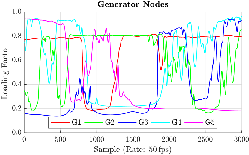
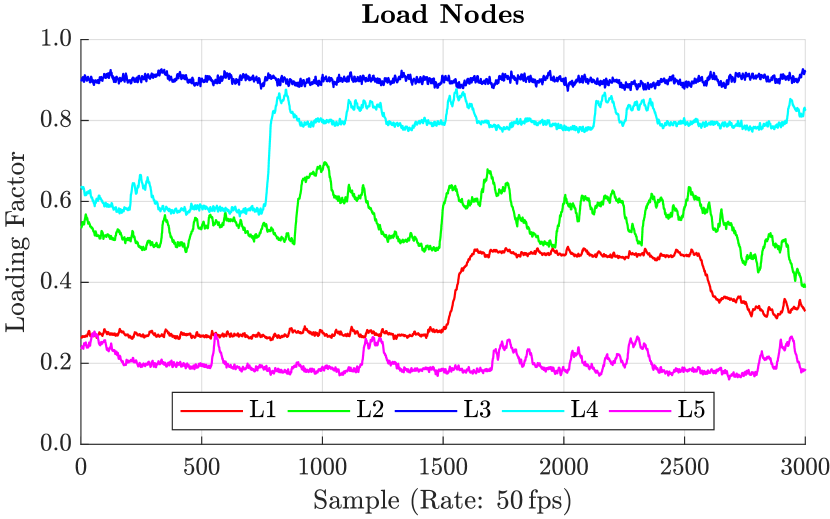
Figure 3: Profiles of the loading factors at the generator and load nodes.

TABLE III: Condition number of the power-flow Jacobian matrix $\boldsymbol{\mathbf{J}}$.

Reduction Step	0	1	2	3	4	5
$\operatorname{cond}(\boldsymbol{\mathbf{J}})$	6.9E3	6.0E3	5.2E3	4.5E3	3.7E3	3.2E3

Reduction Step	6	7	8	9	10
$\operatorname{cond}(\boldsymbol{\mathbf{J}})$	2.5E3	2.1E3	1.6E3	8.5E2	4.9E2

TABLE IV: Condition number of the estimator gain matrix $\boldsymbol{\mathbf{G}}$.

Reduction Step	0	1	2	3	4	5
$\operatorname{cond}(\boldsymbol{\mathbf{G}})$	8.0E9	7.3E9	6.8E9	6.2E9	5.7E9	5.2E9

Reduction Step	6	7	8	9	10
$\operatorname{cond}(\boldsymbol{\mathbf{G}})$	4.7E9	4.1E9	3.4E9	4.4E8	3.3E4

V-B Power-Flow Study

For the NRM, the convergence tolerance is set to $\varepsilon=10^{-8}$, and positive-sequence voltage phasors of magnitude 1 are used as initial points. Convergence is reached after 4–5 iterations. The key performance indicators of the NRM are the condition number of the Jacobian matrix (Tab. III) and the execution time (Fig. 4). Through steps 0–10 of KR (i.e., from the original to the fully reduced system), the condition number improves by a factor of 14, and the median execution time by a factor of 5.

V-C State Estimation

For SE, it is supposed that all slack and resource nodes are equipped with Phasor Measurement Units (PMUs), which measure the phase-to-ground voltages and injected currents in all phases. Moreover, all remaining zero-injection nodes are treated as virtual measurements. The PMUs have a Full-Scale Range (FSR) of 20 kV (RMS) for the voltage phasors and 100 A (RMS) for the current phasors. The standard deviations of the measurement noise are $10^{-3}$ pu (w.r.t. the FSR) for the magnitudes and $1.5\cdot 10^{-3}$ rad for the angles. These values are typical for class 0.1 of voltage/current instrument transformers [36, 37]. For the virtual measurements, these standard deviations are set 100 times smaller. The PMUs are emulated by polluting the voltage phasors obtained in the PFS with suitably scaled white Gaussian noise.

The performance indicators of the WLSR are the condition number of the gain matrix (Tab. IV) and the execution time (Fig. 5). From step 0 to step 10 of KR, the condition number improves by 5 orders of magnitude (this number depends on the assumed standard deviations of the virtual measurements, see [32]), and the median execution time by a factor of 40.

V-D Voltage Stability Assessment

For the VSA, only the loading factors of the load nodes are varied. The CM uses a convergence tolerance of $\varepsilon=10^{-8}$ and a step size of $\sigma=10^{-1}$. The key performance indicators of the HCM are the number of continuation steps (Fig. 6) and the execution time (Fig. 7). Through the application of KR, the number of continuation steps is approximately halved, and the median execution time is reduced by a factor of 10.

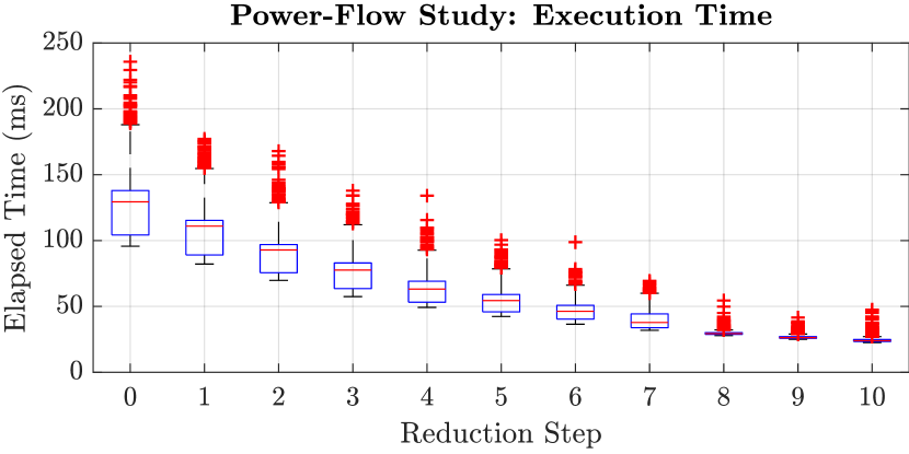
Figure 4: Execution time of the NRM used for PFS.

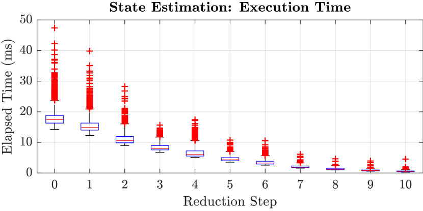
Figure 5: Execution time of the linear WLSR used for SE.

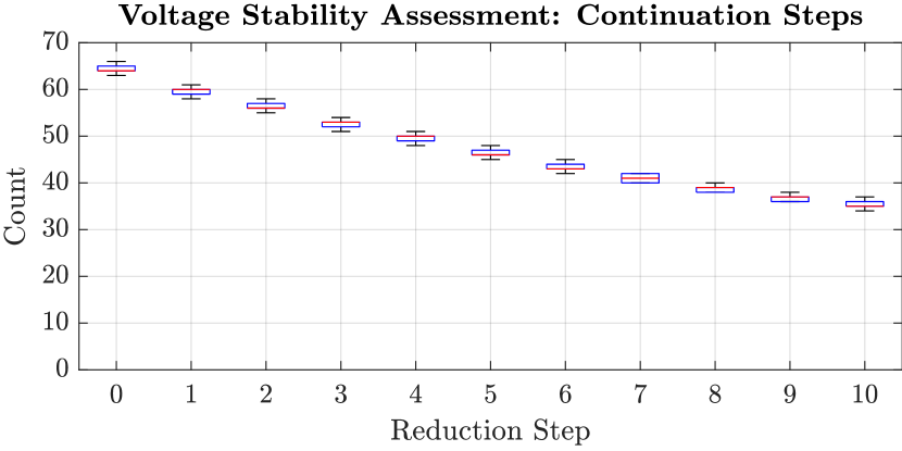
Figure 6: Number of steps of the homotopy CM used for VSA.

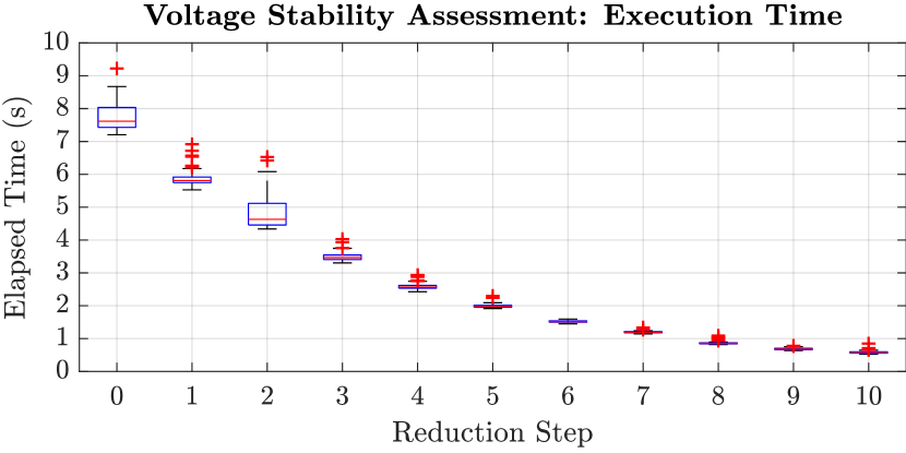
Figure 7: Execution time of the homotopy CM used for VSA.

VI Conclusion

This paper examined the impact of KR on the performance of state-of-the-art numerical methods applied to the analysis of unbalanced polyphase power systems. Namely, the classical applications PFS, SE, and VSA were considered. To this end, the NRM, linear WLSR, and homotopy CM were implemented in MATLAB. The impact of KR on the performance of these methods was assessed using a reproducible test system, from which the zero-injection nodes were successively eliminated. Through the application of KR, the condition number of the power-flow Jacobian matrix was improved by a factor of 14, and the condition number of the estimator gain matrix by 5 orders of magnitude. The median execution times of the NRM, WLSR, and CM were reduced by factors of 5, 40, and 10. These results confirm the applicability and usefulness of KR for the analysis of unbalanced polyphase power systems.

References

- [1] G. Kron, Tensors for Circuits, 2nd ed. New York City, NY, USA: Dover, 1959.
- [2] F. Dörfler and F. Bullo, “Kron reduction of graphs with applications to electrical networks,” IEEE Trans. Circuits Syst. I: Reg. Papers, vol. 60, no. 1, pp. 150–163, Jan. 2013.
- [3] A. M. Kettner and M. Paolone, “On the properties of the power systems nodal admittance matrix,” IEEE Trans. Power Syst., vol. 33, no. 1, pp. 1130–1131, Jan. 2018.
- [4] ——, “On the properties of the compound nodal admittance matrix of polyphase power systems,” IEEE Trans. Power Syst., Accepted for publication. DOI: 10.1109/TPWRS.2018.2863671.
- [5] C. L. Fortescue, “Method of symmetrical coordinates applied to the solution of polyphase networks,” Trans. AIEE, vol. 37, no. 2, pp. 1027–1140, Jun. 1918.
- [6] B. Stott, “Review of load-flow calculation methods,” Proc. IEEE, vol. 62, no. 7, pp. 916–929, Jul. 1974.
- [7] J. Meisel and R. D. Barnard, “Application of fixed-point techniques to load-flow studies,” IEEE Trans. Power App. Syst., vol. 89, no. 1, pp. 136–140, Jan. 1970.
- [8] Y. Wallach, “Gradient methods for load-flow problems,” IEEE Trans. Power App. Syst., no. 5, pp. 1314–1318, May 1968.
- [9] M. A. Laughton, “Analysis of unbalanced polyphase networks by the method of phase coordinates. Part 1: System representation in phase frame of reference,” Proc. IEE, vol. 115, no. 8, pp. 1163–1172, Aug. 1968.
- [10] C. Wang, A. Bernstein, J.-Y. LeBoudec, and M. Paolone, “Explicit conditions on existence and uniqueness of load-flow solutions in distribution networks,” IEEE Trans. Smart Grid, vol. 9, no. 2, pp. 953–962, Mar. 2018.
- [11] S. N. Tiwari and L. P. Singh, “Six-phase (multiphase) power transmission systems: A generalized investigation of the load-flow problem,” Elect. Power Syst. Res., vol. 5, no. 4, pp. 285–297, 1982.
- [12] R. G. Wasley and M. A. Shlash, “Newton-Raphson algorithm for 3-phase load flow,” Proc. IEE, vol. 121, no. 7, pp. 630–638, Jul. 1974.
- [13] I. Kocar, J. Mahseredjian, U. Karaagac, G. Soykan, and O. Saad, “Multiphase load-flow solution for large-scale distribution systems using MANA,” IEEE Trans. Power Del., vol. 29, no. 2, pp. 908–915, Apr. 2014.
- [14] A. J. Monticelli, “Electric power system state estimation,” Proc. IEEE, vol. 88, no. 2, pp. 262–282, Feb. 2000.
- [15] R. E. Larson, W. F. Tinney, and J. Peschon, “State estimation in power systems. Part I: Theory and feasibility,” IEEE Trans. Power App. Syst., no. 3, pp. 345–352, Mar. 1970.
- [16] F. C. Schweppe and J. Wildes, “Power system static-state estimation. Part I: Exact model,” IEEE Trans. Power App. Syst., no. 1, pp. 120–125, Jan. 1970.
- [17] F. C. Schweppe and D. B. Rom, “Power system static-state estimation. Part II: Approximate model,” IEEE Trans. Power App. Syst., no. 1, pp. 125–130, Jan. 1970.
- [18] A. S. Debs and R. E. Larson, “A dynamic estimator for tracking the state of a power system,” IEEE Trans. Power App. Syst., no. 7, pp. 1670–1678, Sep./Oct. 1970.
- [19] M. Paolone, J.-Y. LeBoudec, S. Sarri, and L. Zanni, “Static and recursive PMU-based state estimation processes for transmission and distribution grids,” in Advanced Techniques for Power System Modelling, Control and Stability Analysis, F. Milano, Ed. Stevenage, HRT, UK: IET, 2016.
- [20] A. M. Kettner and M. Paolone, “Sequential discrete Kalman filter for real-time state estimation in power distribution systems: Theory and implementation,” IEEE Trans. Instrum. Meas., vol. 66, no. 9, pp. 2358–2370, Sep. 2017.
- [21] P. S. Kundur et al., “Definition and classification of power system stability,” IEEE Trans. Power Syst., vol. 19, no. 3, pp. 1387–1401, May 2004.
- [22] V. Ajjarapu and C. Christy, “The continuation power flow: A tool for steady-state voltage stability analysis,” IEEE Trans. Power Syst., vol. 7, no. 1, pp. 416–423, Feb. 1992.
- [23] C. A. Cañizares and F. L. Alvarado, “Point-of-collapse and continuation methods for large ac/dc systems,” IEEE Trans. Power Syst., vol. 8, no. 1, pp. 1–8, Feb. 1993.
- [24] H.-D. Chiang, A. J. Flueck, K. S. Shah, and N. J. Balu, “CPFLOW: A practical tool for tracing power system steady-state stationary behavior due to load and generation variations,” IEEE Trans. Power Syst., vol. 10, no. 2, pp. 623–634, May 1995.
- [25] G. D. Irisarri, X. Wang, J. Tong, and S. Mokhtari, “Maximum loadability of power systems using interior-point nonlinear optimization method,” IEEE Trans. Power Syst., vol. 12, no. 1, pp. 162–172, Feb. 1997.
- [26] P.-A. Löf, G. Andersson, and D. J. Hill, “Voltage-stability indices for stressed power systems,” IEEE Trans. Power Syst., vol. 8, no. 1, pp. 326–335, Feb. 1993.
- [27] B. Gao, G. K. Morrison, and P. S. Kundur, “Voltage-stability evaluation using modal analysis,” IEEE Trans. Power Syst., vol. 7, no. 4, pp. 1529–1542, Nov. 1992.
- [28] R. Prada and L. Souza, “Voltage stability and thermal limit: Constraints on the maximum loading of electrical energy distribution feeders,” IEE Proc.–Gener. Transm. Distrib., vol. 145, no. 5, pp. 573–577, 1998.
- [29] H. Sheng and H.-D. Chiang, “CDFLOW: A practical tool for tracing stationary behaviors of general distribution networks,” IEEE Trans. Power Syst., vol. 29, no. 3, pp. 1365–1371, May 2014.
- [30] A. M. Kettner and M. Paolone, “A generalized index for static voltage stability of unbalanced polyphase power systems including Thévenin equivalents and polynomial models,” IEEE Trans. Power Syst., under review, available on https://arxiv.org/abs/1809.09922.
- [31] X.-P. Zhang, P. Ju, and E. Handschin, “Continuation three-phase power flow: A tool for voltage stability analysis of unbalanced three-phase power systems,” IEEE Trans. Power Syst., vol. 20, no. 3, pp. 1320–1329, Aug. 2005.
- [32] L. Zanni, “Power-system state estimation based on PMUs: Static and dynamic approaches, from theory to real implementation,” Ph.D. dissertation, École Polytechnique Fédérale de Lausanne, VD, CH, 2017.
- [33] M. L. Baughman et al., “IEEE 34-node test feeder,” IEEE PES, Tech. Rep., 2004.
- [34] W. W. Price et al., “Load modeling for power-flow and transient-stability computer studies,” IEEE Trans. Power Syst., vol. 3, no. 1, pp. 180–187, Feb. 1988.
- [35] M. Pignati et al., “Real-time state estimation of the EPFL-campus medium-voltage grid by using PMUs,” in Proc. IEEE PES Innovative Smart Grid Techn. Conf. (ISGT), Washington, DC, USA, 2015, pp. 1–5.
- [36] IEC 61869-2:2012, “Instrument transformers, part 2: Additional requirements for current transformers,” International Electrotechnical Commission, Geneva, GE, CH, Standard, 2012.
- [37] IEC 61869-3:2011, “Instrument transformers, part 3: Additional requirements for inductive voltage transformers,” International Electrotechnical Commission, Geneva, GE, CH, Standard, 2011.