Pseudoscalar-Meson Contributions to $g-2$
via Schwinger’s Sum Rule

Abstract:

The Schwinger sum rule is presented as a new promising tool to study the hadronic contributions to the muon anomalous magnetic moment. In particular, we show preliminary results for the light-by-light scattering contribution of pseudoscalar mesons.

1 Introduction

Presently, there is about $4\,\sigma$ discrepancy between the experimental value of the muon anomalous magnetic moment (AMM), $a_{\mu}=\nicefrac{{1}}{{2}}(g-2)_{\mu}$, from BNL-E821 [1] and the Standard Model (SM) prediction [2]:

$$a_{\mu}^{\text{exp.}} = [11\,659\,209.1\pm 6.3]\times 10^{-10},$$ (1a)

$$a_{\mu}^{\text{th.}} = [11\,659\,178.3\pm 4.3]\times 10^{-10},$$ (1b)

where the theory uncertainty is dominated by the hadronic vacuum polarization (HVP) and hadronic light-by-light scattering (HLbL) contributions, see Fig. 1 (a) and (b), respectively:

$$a_{\mu}^{\text{LO HVP}} = [689.46\pm 3.25]\times 10^{-10},\qquad\text{\cite[cite]{[\@@bibref{}{Jegerlehner:2017zsb}{}{}]}}$$ (2a)

$$a_{\mu}^{\text{HLbL}} = [10.34\pm 2.88]\times 10^{-10}.\qquad\text{\cite[cite]{[\@@bibref{}{Jegerlehner:2017gek}{}{}]}}$$ (2b)

The ongoing experiments at Fermilab [5, 6] and J-PARC [7] are expected to improve the experimental precision by a factor of $4$, as well as to provide an important cross check of the previous experiment and of each other. The SM prediction should receive a complementary improvement, meaning the uncertainty of the hadronic contributions should reduce substantially.

The HVP contribution admits a simple dispersive formula:

$$a_{\mu}^{\text{LO HVP}}=\frac{1}{4\pi^{3}}\int_{s_{0}}^{\infty}\mathrm{d}s\,\sigma^{\,e^{+}e^{-}\rightarrow\;\mathrm{hadrons}}(s)\int_{0}^{1}\mathrm{d}x\,\frac{x^{2}(1-x)}{x^{2}+(1-x)(s/m_{\mu}^{2})}\,,$$ (3)

which, to leading order in the fine structure constant $\alpha$, determines it through a single observable: the total cross section of $e^{+}e^{-}\to\mbox{hadrons}$. The common treatment of the HLbL contribution is much more involved and model-dependent (cf., Ref. [4]), which is basically why the relative accuracy of the HLbL value is so much worse than that of the HVP. It is certainly desirable to have an analogue of the simple formula (3) for the HLbL contribution, and that brings us to the subject of this talk.

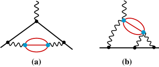
Figure 1: Hadronic contributions to the anomalous magnetic moment: (a) hadronic vacuum polarization and (b) hadronic light-by-light scattering. Hadronic excitations are indicated by red blobs.

2 The Schwinger Sum Rule

As we recently argued [8], the Schwinger sum rule encompasses the dispersive formula (3) for HVP and provides its analogue for HLbL (or, in fact, any other contribution). The Schwinger sum rule reads [9, 10]:

$$a_{\mu} = \frac{m_{\mu}^{2}}{\pi^{2}\alpha}\int_{\nu_{0}}^{\infty}\!\mathrm{d}\nu\,\left[\frac{\sigma_{LT}(\nu,Q^{2})}{Q}\right]_{Q^{2}=0}$$ (4a)

$$= \lim_{Q^{2}\to 0}\frac{8m_{\mu}^{2}}{Q^{2}}\int_{0}^{x_{0}}\mathrm{d}x\;\big{[}g_{1}(x,Q^{2})+g_{2}(x,Q^{2})\big{]},$$ (4b)

where $\sigma_{LT}(\nu,Q^{2})$ is a doubly-polarized photoabsorption cross section, for a given energy $\nu$ and virtuality $Q^{2}$ of the photon. The polarization of the absorbed photon and the target (here, the muon) is rather peculiar in this observable: for the photon it is the interference of the longitudinal and transverse polarization, whereas for the target it is the interference between the positive and negative helicity. One can also understand this observable in terms of the standard spin structure functions, $g_{1}$ and $g_{2}$, see Eq. (4b), with the Bjorken variable $x=Q^{2}/(2m_{\mu}\nu)$.

To see how this sum rule works in QED, recall that the leading photoabsorption process therein is Compton scattering, described by the Feynman diagrams in Fig. 2. The corresponding helicity amplitudes are given by:

$$\mathcal{M}_{\lambda^{\prime}h^{\prime}\lambda h}=-e^{2}\varepsilon_{\lambda^{\prime}}^{\ast\,\mu}(q^{\prime})\varepsilon_{\lambda}^{\nu}(q)\,\bar{\mathpzc{u}}_{h^{\prime}}(p^{\prime})\left[\gamma_{\mu}\,\frac{\not{p}+\not{q}+m_{\mu}}{s-m_{\mu}^{2}}\,\gamma_{\nu}+\gamma_{\nu}\,\frac{\not{p}^{\prime}-\not{q}+m_{\mu}}{u-m_{\mu}^{2}}\,\gamma_{\mu}\right]\mathpzc{u}_{h}(p),$$ (5)

where $\varepsilon(q)$ and $\lambda$ denote the photon polarization-vector and helicity, whereas $\mathpzc{u}(p)$ and $h$ stand for the lepton spinor and helicity; the Mandelstam variables are qiven as usual by $s=(p+q)^{2}$, $u=(p^{\prime}-q)^{2}$, $t=(q-q^{\prime})^{2}$; $e^{2}=4\pi\alpha$. The cross section entering the Schwinger sum rule is then defined via:

$$\frac{\mathrm{d}\sigma_{LT}}{\mathrm{d}t}=\frac{1}{16\pi(s-m_{\mu}^{2})^{2}}\sum_{\lambda^{\prime}h^{\prime}}\frac{1}{\sqrt{2}}\mathrm{Re}\,\big{(}\mathcal{M}^{\ast}_{\lambda^{\prime}h^{\prime}\,1\,\nicefrac{{1}}{{2}}}\mathcal{M}_{\lambda^{\prime}h^{\prime}\,0\,-\nicefrac{{1}}{{2}}}\big{)}.$$ (6)

Upon integrating over $t$, we obtain the total $LT$ cross section for the tree-level (virtual) Compton scattering:

$$\sigma_{LT}(\nu,Q^{2})=\frac{\pi\alpha^{2}Q\,(s-m_{\mu}^{2})^{2}}{4m_{\mu}^{3}\nu^{2}\big{(}\nu^{2}+Q^{2}\big{)}}\left(-2-\frac{m_{\mu}(m_{\mu}+\nu)}{s}+\frac{3m_{\mu}+2\nu}{\sqrt{\nu^{2}+Q^{2}}}\,\mathrm{arccoth}\frac{m_{\mu}+\nu}{\sqrt{\nu^{2}+Q^{2}}}\right),$$ (7)

with $\nu=p\cdot q/m_{\mu}=(s-m_{\mu}^{2}+Q^{2})/2m_{\mu}$, $Q^{2}=-q^{2}$. Substituting this expression into the Schwinger sum rule, we reproduce another famous result of Julian Schwinger: $\alpha/2\pi$.

Figure 2: Tree-level Compton scattering diagrams.

3 Unified Treatment of Hadronic Contributions

To evaluate the impact of a given mechanism on $a_{\mu}$ via the Schwinger sum rule, we need to measure its effect on the photoabsorption cross section $\sigma_{LT}$. There are two fundamentally different ways in which hadrons affect the photoabsorption on a lepton:

• hadron photoproduction, e.g., Fig. 3 (a) and (b);

• hadronic effects in the electromagnetic channels, e.g., Fig. 3 (c) and (d).

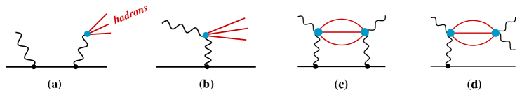
Figure 3: Different channels contributing to the photoabsorption process: hadron photoproduction through timelike Compton scattering (a) or the Primakoff mechanism (b), and hadronic light-by-light contributions to the Compton scattering (c, d) (crossed diagrams omitted).

The first type of contributions can in principle be measured experimentally. They begin to contribute to $\sigma_{LT}$ at $\mathcal{O}(\alpha^{3})$, and hence are of $\mathcal{O}(\alpha^{2})$ in $a_{\mu}$. As shown in Ref. [8], the mechanism of Fig. 3 (a) (timelike Compton scattering) by itself yields exactly the leading-order HVP formula (3). The mechanism of Fig. 3 (b) (Primakoff) by itself yields a vanishing contribution to $a_{\mu}$ [11], which can be proven exactly using the sum rules for light-by-light scattering (see, e.g., [12]). The Primakoff mechanism may contribute in the interference with subleading effects, as will be considered below for the pseudoscalar-meson production, see Fig. 5.

In evaluating the hadronic effects of type (ii), which to $\mathcal{O}(\alpha^{3})$ in $a_{\mu}$ are given by the interference of the diagrams in Fig. 3 (c, d) with the tree-level QED diagrams, one faces the same sort of problem as in the evaluation of the entire HLbL contribution Fig. 1(b), albeit at less than two-loop level. The reduction in number of loops provides a significant simplification and should be helpful in a better determination of the total HLbL contribution.

4 Pseudoscalar-Meson Contribution

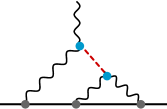
Figure 4: Single-meson (red dashed line) contribution to the anomalous magnetic moment.

The neutral pseudoscalar mesons $\pi^{0}$, $\eta$ and $\eta^{\prime}$ play a significant role in the HLbL contribution, see Fig. 4. The model evaluations of the so-called “pseudoscalar-pole” contribution may differ depending on what is used for the meson transition form factors (or, whether they should be used in both vertices or just one). The most commonly quoted values are:

$$a_{\mu}^{\text{PS-pole}} = 8.3\pm 1.2\times 10^{-10}\qquad\text{Knech \& Nyffeler \cite[cite]{[\@@bibref{}{Knecht:2001qf}{}{}]},}$$ (8a)

$$a_{\mu}^{\text{PS-pole}} = 11.4\pm 1.0\times 10^{-10}\qquad\text{Melnikov \& Vainshtein \cite[cite]{[\@@bibref{}{Melnikov:2003xd}{}{}]}.}$$ (8b)

The most recent value for the dominant $\pi^{0}$-pole contribution [15]:

$$a_{\mu}^{\pi^{0}\text{-pole}}=6.26\,^{+0.30}_{-0.25}\times 10^{-10},$$ (9)

concurs with the first of the two calculations in Eq. (8).

It is interesting to see whether the Schwinger sum-rule approach can tell us something new. To leading order in $\alpha$, we need to consider the following two hadronic channels: $\gamma\mu\rightarrow\mu\pi^{0}$ and $\gamma\mu\rightarrow\mu\pi^{0}\gamma$, for each of pseudoscalars. Here, we present results for the calculation of the first channel: $\gamma\mu\rightarrow\mu\,(\pi^{0},\eta,\eta^{\prime})$, see Fig. 5. The same calculation will apply to the electron AMM, $a_{e}$.

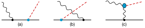
Figure 5: Diagrams contributing to the process of pseudoscalar-meson production off the muon.

In order to compute the diagrams in Fig. 5, we first of all need to specify how a pseudoscalar meson couples to photons and leptons. We use the following couplings:

$$\Gamma^{\mu\nu}_{\pi\gamma\gamma}(q,q^{\prime}) = -ie^{2}F_{\pi\gamma^{*}\gamma^{*}}(q^{2},q^{\prime\,2})\,\epsilon^{\mu\nu\alpha\beta}q_{\alpha}q^{\prime}_{\beta},$$ (10a)

$$\Gamma_{\pi\ell\ell} = -F_{\pi\ell\ell}(M_{\pi}^{2},m^{2},m^{2})\,\gamma_{5},$$ (10b)

each characterized by a form factor. For the coupling to photons, it is the standard transition form factor. Here, the momentum $q$ and the index $\nu$ describe the incoming photon, $q^{\prime}$ and $\mu$ the outgoing photon.

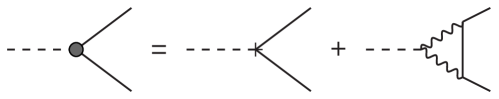
Figure 6: Leading contributions to the pseudoscalar-lepton-lepton interaction.

For the $\pi\ell\ell$ form factor (where $\ell$ stands for a lepton with mass $m$ and $\pi$ for a pseudoscalar meson with respective mass $M_{\pi}$), we use the well-known dispersion relation [16, 17] (resulting from the diagrams in Fig. 6):

$$F_{\pi\ell\ell}(q^{2}) \equiv F_{\pi\ell\ell}(q^{2},m^{2},m^{2})=F_{\pi\ell\ell}(0)+\frac{q^{2}}{\pi}\int_{0}^{\infty}\!\mathrm{d}s\,\frac{\mathrm{Im}\,F_{\pi\ell\ell}(s)}{(s-q^{2})s},$$ (11a)

$$\mathrm{Im}\,F_{\pi\ell\ell}(s) = -\frac{\alpha^{2}m}{2\pi f_{\pi}}\frac{\operatorname{arccosh}(\sqrt{s}/2m)}{\sqrt{1-4m^{2}/s}},$$ (11b)

$$F_{\pi\ell\ell}(0) = \frac{\alpha^{2}m}{2\pi^{2}f_{\pi}}\Big{[}{\mathcal{A}}({\Lambda})+3\ln\frac{m}{{\Lambda}}\Big{]},$$ (11c)

where ${\Lambda}$ is the renormalization scale, and ${\mathcal{A}}$ is a pion-lepton low-energy constant. We evaluate ${\mathcal{A}}$ analogously to Ref. [18, Eq. (10) and (11)], where we use the LMD+V model for the pion transition form factor [13, Eq. (4.4)] and VMD models for the eta and eta-prime transition form factors [19, Eq. (37)]. In addition, we make use of the experimentally known decay widths [20]:

$$\Gamma(\pi^{0}\to e^{+}e^{-}) = 0.499(28)\,\upmu\text{eV},$$ (12a)

$$\Gamma(\eta\to\mu^{+}\mu^{-}) = 7.6(1.1)\,\text{meV},$$ (12b)

which are related to the $\pi\ell\ell$ form factor in the following way [21]:

$$\Gamma(\pi\to\ell^{+}\ell^{-})=\frac{M_{\pi}}{8\pi}\sqrt{1-\frac{4m^{2}}{M_{\pi}^{2}}}\,\big{|}F_{\pi\ell\ell}(M_{\pi}^{2},m^{2},m^{2})\big{|}^{2},$$ (13)

and analogously for the other leptonic decays of pseudoscalar mesons. The resulting couplings are listed in Table 1, where the errors stem from the decay widths in Eq. (12).

Table 1: Coupling strengths of pseudoscalar-muon-muon interactions.

	$\pi^{0}$	$\eta$	$\eta^{\prime}$
${\mathcal{A}}(m)$	$-5.4^{\,+1.0}_{\,-1.2}$	$-6.9_{\,-0.8}^{\,+1.1}$	$-6.0$
$\mathrm{Re}\left[F_{\pi\ell\ell}(M_{\pi}^{2},m^{2},m^{2})\right]\times 10^{7}$	$-145^{\,+32}_{\,-36}$	$-98_{\,-24}^{\,+33}$	$-11$

The interference between the diagrams Fig. 5 (a, b) and Fig. 5 (c), needed to evaluate the $\mathcal{O}(\alpha^{3})$ contribution to $a_{\mu}$, gives the following expression (omitting helicities):

$$|\mathcal{M}|^{2}_{\mathrm{interf.}} = ie^{4}\,\mathrm{Re}\left[F_{\pi\ell\ell}(M_{\pi}^{2},m_{\mu}^{2},m_{\mu}^{2})\right]\,\frac{F_{\pi\gamma^{*}\gamma^{*}}(-Q^{2},t)}{t}\,\epsilon^{\mu\nu\alpha\beta}q_{\alpha}\left(p^{\prime}-p\right)_{\beta}$$

$$\times \left\{\varepsilon^{*}_{\nu}(q)\;\bar{\mathpzc{u}}(p)\gamma_{\mu}\mathpzc{u}(p^{\prime})\;\bar{\mathpzc{u}}(p^{\prime})\left[\gamma_{5}\,\frac{\not{p}+\not{q}+m_{\mu}}{s-m_{\mu}^{2}}\,\not{\varepsilon}(q)+\not{\varepsilon}(q)\,\frac{\not{p}^{\prime}-\not{q}+m_{\mu}}{u-m_{\mu}^{2}}\,\gamma_{5}\right]\mathpzc{u}(p)\right.$$

$$+ \left.\bar{\mathpzc{u}}(p)\left[\not{\varepsilon}^{*}(q)\,\frac{\not{p}+\not{q}+m_{\mu}}{s-m_{\mu}^{2}}\,\gamma_{5}+\gamma_{5}\,\frac{\not{p^{\prime}}-\not{q}+m_{\mu}}{u-m_{\mu}^{2}}\,\not{\varepsilon}^{*}(q)\right]\mathpzc{u}(p^{\prime})\;\bar{\mathpzc{u}}(p^{\prime})\gamma_{\mu}\mathpzc{u}(p)\;\varepsilon_{\nu}(q)\right\},$$

where $p$ ($p^{\prime}$) is the initial (final) lepton momentum, $q$ is the incoming photon momentum, and the Mandelstam variables are defined as usual. Substituting this into Eq. (6), we obtain the differential cross section, which in the limit of $Q^{2}\to 0$ takes the following form:

$$\left[\frac{1}{Q}\frac{\mathrm{d}\sigma_{LT}}{\mathrm{d}t}\right]_{Q^{2}=0} = \frac{\alpha^{2}\pi}{8m_{\mu}^{2}}\,F_{\pi\,\gamma^{*}\gamma^{*}}(t,0)\,\mathrm{Re}\left[F_{\pi\ell\ell}(M_{\pi}^{2},m_{\mu}^{2},m_{\mu}^{2})\right]\frac{1}{t(s-m_{\mu}^{2})(u-m_{\mu}^{2})\nu^{4}}$$

$$\times \Big{\{}m_{\mu}^{2}M_{\pi}^{4}\left(M_{\pi}^{2}-2\nu^{2}\right)-t^{3}\,m_{\mu}\left(m_{\mu}+2\nu\right)$$

$$\quad-\;t\left[m_{\mu}^{2}\left(8\nu^{4}+3M_{\pi}^{4}-8\nu^{2}M_{\pi}^{2}\right)+2\nu\,m_{\mu}M_{\pi}^{2}\left(2\nu^{2}+M_{\pi}^{2}\right)-2\nu^{2}M_{\pi}^{4}\right]$$

$$\quad+\;t^{2}\left[3m_{\mu}^{2}\left(M_{\pi}^{2}-2\nu^{2}\right)+4\nu m_{\mu}\left(M_{\pi}^{2}-\nu^{2}\right)-2\nu^{2}M_{\pi}^{2}\right]\Big{\}}.$$

To obtain the integrated cross section, we integrate within the following interval:

$$t_{\begin{subarray}{c}\text{max}\\ \text{min}\end{subarray}}=M_{\pi}^{2}-(s-m_{\mu}^{2})\big{[}\beta(s)\mp\lambda(s)\big{]},$$ (16)

with $\beta(s)=(s-m_{\mu}^{2}+M_{\pi}^{2})/2s$, $\,\lambda(s)=(1/2s)\sqrt{[s-(M_{\pi}+m_{\mu})^{2}][s-(M_{\pi}-m_{\mu})^{2}]}$.

We are now left to evaluate the sum rule integral, Eq. (4), with the photoabsorption cross section derived above, starting from the pseudoscalar-production threshold ($Q^{2}=0$):

$$\nu_{0}=M_{\pi}\left(1+\frac{M_{\pi}}{2m_{\mu}}\right).$$ (17)

Our results for the contribution of the pseudoscalar-meson production channel to $a_{\mu}$, derived via the Schwinger sum rule, are shown in Table 2. The errors for the $\pi^{0}$ and $\eta$ channels are propagated from the pseudoscalar-muon-muon couplings in Table 1. For the contribution of the $\eta^{\prime}$ production, we assigned a $33\%$ error, similar to the maximal error found for the $\eta$ production. Note that in our calculation we are neglecting the effect of off-shell muons in Fig. 5 (a, b), as well as the diagram in Fig. 7.

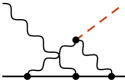
Figure 7: Subleading mechanism accompanying the single-meson photoproduction.

Table 2: Contribution of the pseudoscalar-meson production channel to $a_{\mu}$ in units of $10^{-10}$.

$\gamma\ell\rightarrow\ell\pi^{0}$	$\gamma\ell\rightarrow\ell\eta$	$\gamma\ell\rightarrow\ell\eta^{\prime}$	$\gamma\ell\rightarrow\ell\,(\pi^{0},\eta,\eta^{\prime})$
$16.6^{\,+4.1}_{\,-3.7}$	$8.5^{\,+2.1}_{\,-2.9}$	$1.0\pm 0.3$	$26.1^{\,+4.6}_{\,-4.7}$

5 Conclusion

The Schwinger sum rule provides a dispersive data-driven approach to calculating the hadronic contributions in lepton $g-2$. It encompasses the simple dispersive formula for the HVP contribution, Eq. (3), and allows to treat the others (e.g, the HLbL contribution) on similar footing. The required data on the doubly-polarized photoabsorption cross section $\sigma_{LT}$, which should be used in the sum rule as input, are not presently available. In the absence of data, we are setting up a model for the hadron photoproduction process on the muon.

We have so far evaluated the contribution of the pseudoscalar-meson production channels ($\gamma\mu\rightarrow\mu\,\pi^{0},\mu\eta,\mu\eta^{\prime}$) to the muon $g-2$. More specifically, we have calculated the interference cross section between the diagrams in Fig. 5 (a, b) with the Primakoff diagram in Fig. 5 (c). The resulting contribution to the muon $g-2$, given in Table 2, is a factor $2$ to $3$ larger than the conventional pseudoscalar-pole contributions of Eq. (8) and (9). However, as explained in Sec. 3, the single-meson photoproduction channel is one of four photoabsorption channels contributing to $g-2$ at $\mathcal{O}(\alpha^{3})$. In other words, our results are only a partial $\mathcal{O}(\alpha^{3})$ calculation of the HLbL contribution, and hence, may not be directly comparable to the conventional meson-pole results. Inclusion of the remaining channels might restore the agreement with (at least one of) the conventional calculations.

References

• [1] G. W. Bennett, et al. [Muon g-2 Collaboration], Phys. Rev. D 73, 072003 (2006).
• [2] F. Jegerlehner, Acta Phys. Polon. B 49, 1157 (2018).
• [3] F. Jegerlehner, arXiv:1711.06089 [hep-ph].
• [4] F. Jegerlehner, Springer Tracts Mod. Phys.  274 (2017).
• [5] I. Logashenko, et al. [Muon g-2 Collaboration], J. Phys. Chem. Ref. Data 44, no. 3, 031211 (2015).
• [6] G. Venanzoni [Fermilab E989 Collaboration], Nucl. Part. Phys. Proc.  273-275, 584 (2016).
• [7] M. Otani [E34 Collaboration], JPS Conf. Proc.  8, 025008 (2015).
• [8] F. Hagelstein and V. Pascalutsa, Phys. Rev. Lett.  120, no. 7, 072002 (2018).
• [9] J. S. Schwinger, Proc. Nat. Acad. Sci.  72, 1 (1975); ibid. 72, 1559 (1975) [Acta Phys. Austriaca Suppl.  14, 471 (1975)].
• [10] A. M. Harun ar-Rashid, Nuovo Cim. A 33, 447 (1976).
• [11] F. Hagelstein, V. Pascalutsa and M. Vanderhaeghen, in preparation.
• [12] V. Pascalutsa, V. Pauk and M. Vanderhaeghen, Phys. Rev. D 85, 116001 (2012).
• [13] M. Knecht and A. Nyffeler, Phys. Rev. D 65, 073034 (2002).
• [14] K. Melnikov and A. Vainshtein, Phys. Rev. D 70, 113006 (2004).
• [15] M. Hoferichter, B.-L. Hoid, B. Kubis, S. Leupold and S. P. Schneider, Phys. Rev. Lett. 121, 112002 (2018).
• [16] S. Drell, Il Nuovo Cimento 11, 693-697 (1959).
• [17] L. Ametller, A. Bramon, E. Masso, Phys. Rev. D 30 251 (1984).
• [18] A. E. Dorokhov and M. A. Ivanov, Phys. Rev. D 75 114007 (2007).
• [19] A. Nyffeler, Phys. Rev. D 79, 073012 (2009).
• [20] M. Tanabashi, et al. (PDG), Phys. Rev. D 98, 030001 (2018).
• [21] D. Griffiths, Introduction to Elementary Particles, WILEY-VCH Verlag, 2008.