Confinement-Deconfinement Crossover in the Lattice $\mathbb{C}P^{N-1}$ Model

Abstract

The $\mathbb{C}P^{N-1}$ sigma model at finite temperature is studied using lattice Monte Carlo simulations on $S_{s}^{1}\times S_{\tau}^{1}$ with radii $L_{s}$ and $L_{\tau}$, respectively, where the ratio of the circumferences is taken to be sufficiently large ($L_{s}/L_{\tau}\gg 1$) to simulate the model on $\mathbb{R}\times S^{1}$. We show that the expectation value of the Polyakov loop undergoes a deconfinement crossover as $L_{\tau}$ is decreased, where the peak of the associated susceptibility gets sharper for larger $N$. We find that the global PSU($N$)=SU($N$)$/{\mathbb{Z}}_{N}$ symmetry remains unbroken at “quantum” and “classical” levels for the small and large $L_{\tau}$, respectively: in the small $L_{\tau}$ region for finite $N$, the order parameter fluctuates extensively with its expectation value consistent with zero after taking an ensemble average, while in the large $L_{\tau}$ region the order parameter remains small with little fluctuations. We also calculate the thermal entropy and find that the degrees of freedom in the small $L_{\tau}$ regime are consistent with $N-1$ free complex scalar fields, thereby indicating a good agreement with the prediction from the large-$N$ study for small $L_{\tau}$.

Introduction: The ${\mathbb{C}}P^{N-1}$ sigma model Eichenherr:1978qa ; Witten:1978bc ; DAdda:1978vbw ; DAdda:1978dle is known to show up in various aspects of physics. Originally, the ${\mathbb{C}}P^{N-1}$ model in two dimensions is regarded as a toy model of QCD, since they share various common properties such as asymptotic freedom, confinement and generation of a mass gap. Recently, connections between two dimensional ${\mathbb{C}}P^{N-1}$ models and four dimensional gauge theories have been established: it appears as the low-energy effective theory on a non-Abelian vortex in the non-Abelian gauge-Higgs model Hanany:2003hp ; Auzzi:2003fs ; Eto:2005yh ; Eto:2006cx ; Eto:2006pg ; Tong:2005un ; Eto:2006pg ; Shifman:2007ce as well as dense QCD Nakano:2007dr ; Eto:2009bh ; Eto:2009tr ; Eto:2013hoa , on a long string of Yang-Mills theory Aharony:2013ipa , and of an appropriately compactified Yang-Mills theory Yamazaki:2017ulc . In condensed-matter physics, the ${\mathbb{C}}P^{1}$ model plays an essential role in the research on the low-energy behavior of anti-ferromagnetic spin chains and their extensions Haldane:1982rj , and describes quantum phase transition known as deconfined criticality Senthil:2004aza ; Nogueira:2013oza , while the ${\mathbb{C}}P^{N-1}$ model appears as an $SU(N)$ spin chain Beard:2004jr and also can be realized in ultracold atomic gases Laflamme:2015wma ; Kataoka:2010sh .

Theoretically, non-perturbative properties of the ${\mathbb{C}}P^{N-1}$ model have been studied both analytically by the gap equations with the large-$N$ (mean field) approximation Witten:1978bc ; DAdda:1978vbw ; DAdda:1978dle and by lattice simulations mainly on topological aspects of the model defined on $\mathbb{R}^{2}$ Berg:1981er ; Campostrini:1992ar ; Alles:2000sc ; Flynn:2015uma ; Bruckmann:2015sua ; Bruckmann:2016txt ; Abe:2018loi ; Bruckmann:2018rra ; Bonanno:2018xtd . These analyses are consistent with the Coleman-Mermin-Wagner (CMW) theorem Coleman:1973ci ; Mermin:1966fe forbidding spontaneous breaking of a continuous symmetry in two dimensions, while perturbative analyses are not. Recently, the large-$N$ analyses have been extensively applied to the ${\mathbb{C}}P^{N-1}$ model at finite temperature, or equivalently the model defined on $\mathbb{R}\times S^{1}$ with the periodic boundary conditions (pbc) Monin:2015xwa ; Monin:2016vah (see also the earlier works Hong:1994uv ; Hong:1994te ). However, these studies do not reach a consensus for physics at high temperature (or at small compactification radius) Monin:2015xwa ; Monin:2016vah ; Bolognesi:2019rwq ; Flachi:2019jus (see also Nitta:2017uog ; Nitta:2018lnn ; Nitta:2018yen ; Yoshii:2019yln ) including an analogous case of the model defined on a finite interval Milekhin:2012ca ; Bolognesi:2016zjp ; Milekhin:2016fai ; Betti:2017zcm ; Flachi:2017xat ; Bolognesi:2018njt ; Chernodub:2019nct ; Pavshinkin:2019bed ; Flachi:2019jus , while all studies agree that the physics at low temperature (or at large radius) recovers the CMW theorem. The questions can be summarized as follows: (i) How the order parameter is defined and how its expectation value depends on the compactification period $L_{\tau}$. (ii) How the global PSU($N$)$=$SU($N$)$/{\mathbb{Z}}_{N}$ symmetry is realized for finite $N$. One may naively expect the global symmetry to be broken in the deconfinement phase, where field variables are ordered. It was suggested that the global symmetry is broken in the “deconfinement” phase in the large-$N$ limit Monin:2015xwa ; Monin:2016vah . On the other hand, the CMW theorem forbids the continuous symmetry breaking at least in finite $N$. (iii) How the high temperature behavior changes for finite $N$. In the large-$N$ limit, an explicit high temperature behavior of the free energy was calculated Monin:2015xwa .

In this Letter, we investigate the ${\mathbb{C}}P^{N-1}$ model at finite temperature by the lattice Monte Carlo simulation to solve the above mentioned questions. We also calculate the Polyakov loop expectation value, its susceptibility and the thermal entropy. Our results can be summarized as follows: (1) We adopt the absolute value of the expectation value of the Polyakov loop as a confinement-deconfinement order parameter. We find that its $L_{\tau}$ dependence exhibits a crossover behavior and the peak of its susceptibility gets sharper with $N$ increases, implying a possibility of the phase transition in the large-$N$ limit Monin:2015xwa . (2) We find that the global PSU($N$)=SU($N$)$/{\mathbb{Z}}_{N}$ symmetry remains unbroken at “quantum” and “classical” levels for the small and large $L_{\tau}$, respectively. (3) We calculate the thermal entropy in the small $L_{\tau}$ regime, where the weak-coupling expansion is valid. We show that the result coincides with that for $N-1$ free complex scalar fields, which is in good agreement with the analytical prediction Monin:2015xwa based on the free energy in the large-$N$ limit.

Model and Lattice setup: The continuum bare action of the ${\mathbb{C}}P^{N-1}={\rm SU}(N)/({\rm SU}(N-1)\times{\rm U}(1))$ sigma models (without the topological $\theta$-term) is $S={1\over{2g^{2}}}\int d^{2}x|D_{\mu}\phi|^{2}\,$ with $|\phi|^{2}=1$, $D_{\mu}\phi=(\partial_{\mu}+iA_{\mu})\phi$. Here, $\phi=(\phi^{1},\cdots,\phi^{N})$ is an $N$-component complex scalar field, and $A_{\mu}$ is an auxiliary U($1$) gauge field defined as $A_{\mu}\equiv\frac{i}{2}\bar{\phi}\cdot\overset{\leftrightarrow}{\partial}_{\mu}\phi$. This model has a PSU($N$)=SU($N$)/${\mathbb{Z}}_{N}$ global symmetry, where the ${\mathbb{Z}}_{N}$ center is removed since it coincides with a subgroup of U($1$) gauge symmetry and is redundant.

On the lattice, the action is expressed as Berg:1981er ; Campostrini:1992ar ; Alles:2000sc ; Flynn:2015uma ; Abe:2018loi

$$S=N\beta\sum_{n,\mu}\left(2-\bar{\phi}_{n+\mu}\cdot\phi_{n}\,\lambda_{n,\mu}-\bar{\phi}_{n}\cdot\phi_{n+\mu}\bar{\lambda}_{n,\mu}\right)\,,$$ (1)

where $\phi_{n}$ is an $N$-component complex scalar field satisfying $\bar{\phi relationisone-to-one}_{n}\cdot\phi_{n}=1$ and $\lambda_{n,\mu}$ is a link variable corresponding to the auxiliary U($1$) gauge field ($\lambda_{n,\mu}=e^{iA_{\mu}(n)}$). Here, $n=(n_{x},n_{\tau})$ labels the sites on the lattice and $(n_{x},n_{\tau})$ run as $n_{x}=1,\cdots,N_{s}$ and $n_{\tau}=1,\cdots,N_{\tau}$, respectively. We also note that $N\beta$ corresponds to the inverse of the bare coupling ${1\over{g^{2}}}$. The advantage of this expression is that the fields can be updated locally in Monte Carlo simulation. We here adopt the over-heat-bath algorithm Campostrini:1992ar to update the fields.

The spacetime geometry on the lattice is $\mathbb{T}^{2}=S^{1}_{s}\times S^{1}_{\tau}$, where $S_{s}^{1}$ and $S^{1}_{\tau}$ have the circumferences $L_{s}=N_{s}a$ and $L_{\tau}=N_{\tau}a$, respectively. According to the renormalization group, the following relation between the lattice parameter $\beta$ and the lattice spacing $a$ holds $\Lambda_{\overline{MS}}\,a=(2\pi\beta)^{{2\over{N}}}e^{-2\pi\beta}\,,$ where $\Lambda_{\overline{MS}}$ is defined as a scale at which the renormalized coupling in the $\overline{MS}$ scheme diverges. The lattice $\Lambda$ scale $\Lambda_{lat}$ depends on the explicit form of the lattice action. Comparing $\Lambda_{\overline{MS}}$ in Ref. Campostrini:1992ar and $\Lambda_{lat}$ for Eq.(1), we find

$$\Lambda_{lat}\,a={1\over{\sqrt{32}}}(2\pi\beta)^{2\over{N}}e^{-2\pi\beta-{\pi\over{2N}}}\,.$$ (2)

It gives $a$ for a given $\beta$ for each $N$ with $\Lambda_{lat}$ as a reference scale. This relation is valid for $\beta\gtrsim 1/(\pi N)$, which is comfortably satisfied in this work.

We confirm that the action density $\langle E\rangle=\langle 2-\bar{\phi}_{n+\mu}\cdot\phi_{n}\lambda_{n,\mu}-\bar{\phi}_{n}\cdot\phi_{n+\mu}\bar{\lambda}_{n,\mu}\rangle$ in our numerical calculations is consistent with the results based on the strong-coupling expansion $\langle E\rangle\approx 2(1-\beta)$ for low $\beta$ ($\beta\lesssim 0.4$), while it agrees with the result based on weak-coupling expansion $\langle E\rangle\approx 1/(2\beta)$ for high $\beta$ ($2.0\lesssim\beta$).

By setting $L_{s}\gg L_{\tau}$, we can approximately simulate the model on $\mathbb{R}\times S^{1}$, where the compactified circumference $L_{\tau}$ is interpreted as an inverse temperature $1/T$. We will mainly use $L_{\tau}$ in this Letter, where the smaller $L_{\tau}$ (the higher $\beta$ with fixed $N_{\tau}$) corresponds to the higher $T$. The lattice size in this work is mainly $(N_{s},N_{\tau})=(200,8)$. We also vary $N_{s}$ between $40$ and $200$ to look into the finite-volume effects. It is notable that the $N_{s}\to\infty$ limit corresponds to a thermodynamic limit, where the model is defined on ${\mathbb{R}}\times S^{1}$ and the genuine phase transition can occur. We adopt parameters as $N=3,5,10,20$ and $0.1\leq\beta\leq 3.9$.

Deconfinement and Polyakov loop: The ground state expectation value of the Wilson loop $W({\mathcal{C}})={\mathcal{P}}\exp(i\oint_{\mathcal{C}}A)$ is expected to exhibit the exponential area law and perimeter law for a large rectangle with space $\hat{R}$ and Euclidean time $\hat{T}$

$$\langle W({\mathcal{C}})\rangle\,=\,Ce^{-\sigma\hat{R}\hat{T}-\rho(\hat{R}+\hat{T})}\,,$$ (3)

with the Abelian string tension $\sigma\geq 0$, a constant $\rho\geq 0$ of the perimeter term, and a constant $C$. The confinement of electrically charged particles is defined by the nonvanishing $\sigma$. Actually, on lattice simulation with a large $N_{s}=N_{\tau}$, the value of the string tension can be calculated by the large Wilson loop Campostrini:1992ar . If we compactify the spacetime as $\tau\sim\tau+L_{\tau}$ and impose the PBC, the Wilson loop becomes a correlator of Polyakov loops, $P(x)\equiv{\mathcal{P}}\exp(i\int_{0}^{L_{\tau}}d\tau A_{\tau})_{x}$ at $x$ ,

$$\langle W({\mathcal{C}})\rangle\,=\,\langle P(\hat{R})P^{\dagger}(0)\rangle.$$ (4)

Since the Wilson loop (3) satisfies the clustering property $\langle P(\hat{R})P^{\dagger}(0)\rangle\to|\langle P\rangle|^{2}$ in $\hat{R}\rightarrow\infty$, the confinement $\sigma\not=0$ necessitates the vanishing Polyakov loop $\langle P\rangle=0$. The ground state expectation value of the Polyakov loop $\langle P\rangle$ is a better observable for the confinement-deconfinement transition in the $L_{\tau}\ll L_{s}$ system, where taking the large Euclidean time is technically difficult. This situation is parallel to four-dimensional QCD with fundamental quarks.

On the lattice, the Polyakov loop is expressed as the product of the link variable,

$$P\equiv{1\over{N_{s}}}\sum_{n_{x}}\prod_{n_{\tau}}\lambda_{n,\tau}.$$ (5)

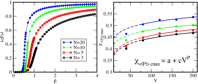
Figure 1: (Left) The absolute value of expectation value of Polyakov loop $|\langle P\rangle|$ as a function of $\beta$ (Right) The volume dependences of the maximal peak height of the Polyakov loop susceptibility for each $N$ by varying $N_{s}$ as $N_{s}=40,80,120,160,200$ with $N_{\tau}=8$.

The results for $|\langle P\rangle|$ as a function of $\beta$ for $N=3,5,10,20$ are summarized in the left panel of Fig. 1. Here, the lattice parameters are fixed by ($N_{s},N_{\tau}$) $=$ ($200,8$). It clearly shows $|\langle P\rangle|\approx 0$ for low $\beta$ (large $L_{\tau}$) and $|\langle P\rangle|\not=0$ for high $\beta$ (small $L_{\tau}$). For intermediate $\beta$, the value of $|\langle P\rangle|$ gradually increases especially for small $N$, as is consistent with a crossover behavior.

The corresponding susceptibility of $\langle|P|\rangle$ has a peak, and then we define the critical length (or the critical inverse temperature) for each $N$ from the peak position of $\beta$. We also investigate the heat capacity, $C_{v}=(E-\langle E\rangle)^{2}N_{\tau}^{2}$, where $E$ denotes the action density. The heat capacity for each $N$ has the peak at the same value of $\beta$ with the one for the susceptibility of $\langle|P|\rangle$.

To see the strength of the transition more clearly, we also investigate the volume dependence of the peak value of the Polyakov loop susceptibility, $\chi_{\langle|P|\rangle}=V(\langle|P|^{2}\rangle-\langle|P|\rangle^{2})$, by varying $N_{s}$ as $N_{s}=40,80,120,160,200$ with $N_{\tau}=8$ fixed. We study the scaling with respect to volume, $V=N_{s}$. We fit the four data points with the large volume, $N_{s}=80$–$200$, by a function $\chi_{\langle|P|\rangle,{\rm max}}\,=\,a+cV^{p}\,$ as shown in the right panel of Fig. 1. The best fit values of the exponent are $p=0.056(7),0.058(7),0.052(7),$ and $0.043(8)$ for $N=3,5,10$, and $20$, respectively. Since it is known that $p=1$ indicates the first-order transition while $0<p<1$ indicates the second-order or crossover transitions Fukugita:1990vu , this result supports our argument that the order of the transition is crossover for finite $N$. Furthermore, all results of the exponent are consistent with each other within $2$–$\sigma$ statistical error, so that we conclude that there is no clear $N$-dependence for the strength of the transition in these finite $N$ analyses.

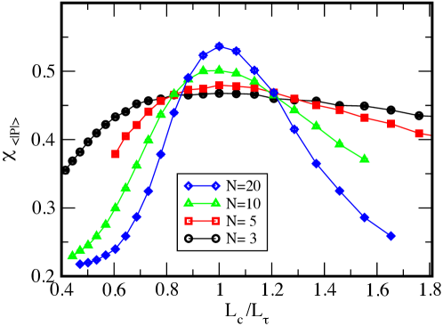
Figure 2: The susceptibility of the expectation value of absolute value of Polyakov loop $\langle|P|\rangle$ as a function of $L_{c}/L_{\tau}$ for $N=3,5,10,20$ with ($N_{s},N_{\tau}$)$=$($200,8$).

On the other hand, in the large-$N$ limit, we first take the large-$N$ limit with a finite $L_{\tau}$. To explore the $N$ dependence of the strength of the transition at a finite fixed-volume, the susceptibility of $\langle|P|\rangle$ as a function of a linear scale of $1/L_{\tau}$ is shown in Fig. 2. Here, the critical length ($L_{c}$) for each $N$ is defined from the peak position of $\beta$ with fixed ($N_{s},N_{\tau}$)=($200,8$) simulations, and $\beta$ is translated into the length $L_{\tau}=N_{\tau}a$ via Eq. (2). The $N$ dependence of the susceptibility indicates that the peak is quite broad for small $N$ but it gets sharper as $N$ increases. This result suggests that the order of transition is crossover for finite $N$ while it is possibly transformed into a phase transition in the large-$N$ limit as conjectured in Ref. Monin:2015xwa .

Global PSU($N$) symmetry: It was claimed in Ref. Monin:2015xwa that the deconfinement phase transition is associated with the PSU($N$) symmetry breaking in the large-$N$ analysis while, at finite $N$, the PSU($N$) global symmetry is never broken in two-dimensions even at finite temperature because of the CMW theorem. Now, we found the confinement and deconfinement phases even for finite $N$, then the questions arise: whether the PSU($N$) symmetry exists in the deconfinement phase and, it it exists, how the symmetry is realized in the phase.

To look into this property, we calculate the following $N\times N$ matrix quantity,

$$P^{ij}\equiv\sum_{n}\bar{\phi}^{i}\phi^{j}(n)-{1\over{N}}\delta^{ij}\,,~{}~{}~{}i,j=1,...,N$$ (6)

whose expectation value serves as an order parameter of the PSU($N$) symmetry in the ${\mathbb{C}}P^{N-1}$ model. The distributions of the diagonal components $P^{ii}$ ($i=1,2,3$) with $N=3$ for the confinement phase ($\beta=0.1$) and the deconfinement phase ($\beta=3.9$) are presented in Fig. 3. The horizontal axis stands for the label number of configurations, where we pick up one configuration per $5000$ sweeps.

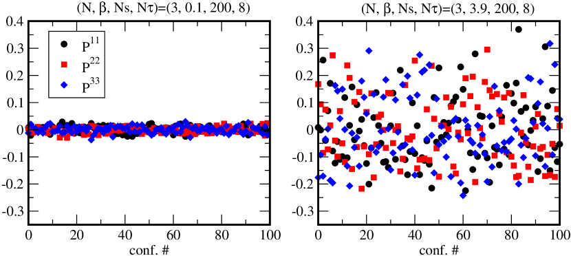
Figure 3: $P^{ii}$ ($i=1,2,3$) with $N=3$ for $\beta=0.1$ (confinement) (left) and $\beta=3.9$ (deconfinement) (right) are shown. The horizontal axis stands for the label number of configurations and we pick up one per $5000$ sweeps.

In the confinement phase, the values of $|P^{ii}|$ are relatively small for all the configurations and lead to $\langle P^{ii}\rangle\approx 0$ as $\langle P^{11}\rangle=-2.80(5808)\times 10^{-5},\langle P^{22}\rangle=3.31(553)\times 10^{-4},\langle P^{33}\rangle=-3.03(589)\times 10^{-4}$. On the other hand, in the deconfinement phase, the values of $P^{ii}$ for some of configurations are far from zero and are distributed broadly. The expectation values for this case is, however, still consistent with zero, where $\langle P^{11}\rangle=-8.22\times 10^{-4},\langle P^{22}\rangle=1.48\times 10^{-6},\langle P^{33}\rangle=8.21\times 10^{-4}$ with $O(10^{-2})$ statistical errors. We can phrase that PSU($N$) symmetry is realized at a “quantum level” in the deconfined phase , in contrast to the confinement phase in which it is realized at a “classical level.” The word “quantum” is to emphasize $P^{ii}$ vanishes only after taking ensemble average while the field variables on each configuration are ordered. We carry out the similar analyses also for $N=5,10,20$ and find no sign of the PSU($N$) symmetry breaking although the fluctuation seems to get larger with $N$. It is still an open question whether or not this global symmetry is broken in the large-$N$ limit.

Thermal entropy density: Now, we numerically find all $N$ components of $\phi^{i}$ are equivalent even in the deconfinement phase, but actual degrees of freedom must be $N-1$ due to one constraint, $|\phi|^{2}=1$. To show it manifestly, let us study the thermal entropy density ($s$), which counts the degrees of freedom of the system, in the deconfinement phase.

In the finite temperature (quenched) QCD, the thermal entropy has been calculated by two independent ways; from the energy-momentum tensor (EMT) and the free energy. It has been confirmed that these approaches give consistent results Asakawa:2013laa . We first focus on the EMT followed by the free energy. We define the following quantities as a lattice EMT:

$$T_{\tau\tau} = 2N\beta(2-\bar{\phi}_{n+\tau}\cdot\phi_{n}\lambda_{n,\tau}-\bar{\phi}_{n}\cdot\phi_{n+\tau}\bar{\lambda}_{n,\tau})$$ (7)

$$-(\mbox{trace part}).$$

$T_{xx}$ can be defined as well. The vacuum expectation value of the trace part is subtracted, in a manner parallel to the lattice EMT for the $O(N)$ sigma model Makino:2014sta ; Makino:2014cxa .

Here, we use the bare coupling constant instead of calculating the renormalized EMT, since it is a good approximation in the weak coupling regime. The thermal entropy density is given by $T_{xx}-T_{\tau\tau}=sT$ with $T\equiv 1/L_{\tau}$ in the thermodynamic limit, where the divergent part of the EMT is cancelled between the two terms.

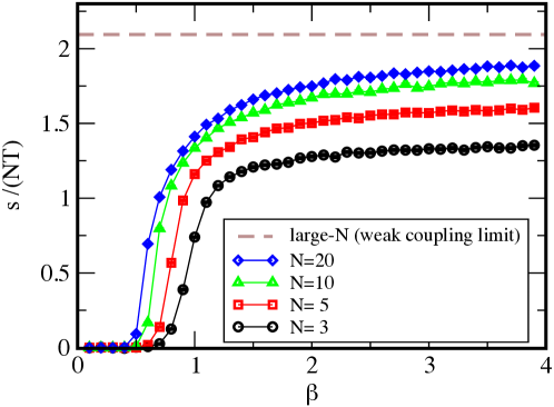
Figure 4: Thermal entropy density for single $\phi$ ($s/(NT)=N_{\tau}^{2}\langle T_{xx}-T_{\tau\tau}\rangle/N$) for $N=3,5,10,20$. The dotted line denotes the large-$N$ results in small $L_{\tau}$ regime, $2\pi/3$.

The results of the thermal entropy density for single scalar field for $N=3,5,10,20$ as a function of $\beta$ are shown in Fig. 4. The thermal entropy density becomes non-zero around a certain $\beta$ corresponding to $L_{c}$ and monotonically grows up in the deconfinement phase. For high-$\beta$ regions, the $\beta$ dependence gets gentler for each $N$, where we fit them by a function $g(\beta)=a+b/\beta$ between $3.0\leq\beta\leq 3.9$. The best fit values of $a$ are $a_{N=3}=1.418(27),a_{N=5}=1.681(26),a_{N=10}=1.889(29),a_{N=20}=2.024(30)$. We then find that the values in the $\beta\rightarrow\infty$ limit are consistent with $2\pi(N-1)/(3N)$.

On the other hand, the free energy density for a free massive complex scalar field in the finite temperature ($T=1/L_{\tau}$) is given by

$$f=\frac{1}{L_{s}L_{\tau}}\sum_{n=-\infty}^{\infty}\log 4\sinh^{2}\frac{\omega_{n}L_{\tau}}{2}-f_{0}$$ (8)

from the analytical calculation (see Appendix. A). Here, $\omega_{n}^{2}=\left(\frac{2\pi n}{L_{s}}\right)^{2}+m^{2}$ and $f_{0}$ denotes the counter term which cancels the UV divergence. Then, the thermal entropy density in the massless and thermodynamic limit ($L_{s}\rightarrow\infty$) is given by $s/T=-\frac{1}{T}\frac{\partial f}{\partial T}=\frac{2\pi}{3}$ for a single complex scalar field. Our numerical results indicate that the actual degree of freedom of the $\mathbb{C}P^{N-1}$ model is ($N-1$) massless free complex scalar fields in the deconfinement phase. Furthermore, the large-$N$ limit of our results is consistent with the prediction calculated from the free energy for the large-$N$ limit in small $L_{\tau}$ regime, $f=-\frac{N\pi}{3L^{2}_{\tau}}$ Monin:2015xwa ; Luscher:2004ib ; Teper:2009uf ; Caselle:2015tza using similar calculations.

Summary and Discussion: In this Letter, we have reported the results on the non-perturbative aspects of the ${\mathbb{C}}P^{N-1}$ model on $S^{1}({\rm large})\times S^{1}({\rm small})$: We have found a confinement-deconfinement crossover by calculating the $L_{\tau}$ dependence of the expectation value of the Polyakov-loop, where the peaks of its susceptibility get shaper as $N$ increases. We have clearly shown that the global PSU($N$)=SU($N$)$/{\mathbb{Z}}_{N}$ symmetry remains unbroken at “quantum” and “classical” levels for the small and large $L_{\tau}$, respectively, consistent with the CMW theorem. We have obtained the thermal entropy in small $L_{\tau}$ regime for small and large $N$, and have shown that the large $N$ values agree with the small $L_{\tau}$ results of the large-$N$ approximation.

Our results give a new insight on the phase diagram of the $\mathbb{C}P^{N-1}$ model. Furthermore, since some of the conjectures we have discussed originate in four-dimensional gauge theories, our results also would give significant implications to four-dimensional gauge theories.

As a future avenue, our formalism can be extended to the model with different geometries and/or boundary conditions, such as the model on $\mathbb{R}\times S^{1}$ with $\mathbb{Z}_{N}$ twisted boundary conditions, where $\mathbb{Z}_{N}$ symmetry is exact Dunne:2012ae ; Dunne:2012zk ; Tanizaki:2017qhf , and the model on a finite interval for which the Casimir effect is extensively argued Milekhin:2012ca ; Bolognesi:2016zjp ; Milekhin:2016fai ; Betti:2017zcm ; Flachi:2017xat ; Bolognesi:2018njt ; Chernodub:2019nct ; Pavshinkin:2019bed ; Flachi:2019jus . For the former, whether it undergoes a first-order phase transition or has adiabatic continuity of the vacuum structure Sulejmanpasic:2016llc and whether fractional instantons have physical consequences Eto:2004rz ; Eto:2006mz ; Eto:2006pg ; Bruckmann:2007zh ; Brendel:2009mp ; Nitta:2014vpa ; Nitta:2015tua ; Bruckmann:2018rra ; Itou:2018wkm ; Misumi:2014jua ; Misumi:2015dua ; Wan:2018zql in the model are questions attracting a great deal of attention in terms of the resurgence theory of the models Dunne:2012ae ; Dunne:2012zk ; Misumi:2014jua ; Misumi:2015dua ; Buividovich:2015oju ; Fujimori:2016ljw ; Fujimori:2017oab ; Fujimori:2017osz ; Dorigoni:2017smz ; Fujimori:2018kqp .

I Appendix A: Thermal entropy of a free massive scalar field

In this appendix, we calculate the thermal entropy of a free massive scalar field

$$S=\int d^{2}x\,(|\partial_{\mu}\phi|^{2}+m^{2}|\phi|^{2}).$$ (9)

On a torus with periods $(L_{\tau},L_{s})$, this model can be regarded as a collection of infinitely many 2D harmonic oscillators with frequencies $\omega_{n}^{2}=\left(\frac{2\pi n}{L_{s}}\right)^{2}+m^{2}$ at temperature $T=1/L_{\tau}$, so that the partition function is given by

$$Z=\prod_{n=-\infty}^{\infty}\frac{1}{4\sinh^{2}\frac{L_{\tau}\omega_{n}}{2}}.$$ (10)

The free energy density can be obtained from $Z=e^{-L_{\tau}L_{s}f}$ as

$$f=\frac{1}{L_{\tau}L_{s}}\sum_{n=-\infty}^{\infty}\log 4\sinh^{2}\frac{L_{\tau}\omega_{n}}{2}+m^{2}-f_{0},$$ (11)

where the last term denotes the counter term which cancels the UV divergence. In the infinite volume limit $L_{s}\rightarrow\infty$, the summation over the Kaluza-Klein momentum is replaced by the momentum integration

$$f=\frac{1}{L_{\tau}}\int\frac{dk}{2\pi}\log 4\sinh^{2}\frac{L_{\tau}\sqrt{k^{2}+m^{2}}}{2}-f_{0}.$$ (12)

The energy density can be calculated from this free energy as

$$\epsilon\,=\,\frac{\partial}{\partial L_{\tau}}(L_{\tau}f)=\int\frac{dk}{2\pi}\sqrt{k^{2}+m^{2}}\,\coth{\frac{L_{\tau}}{2}\sqrt{k^{2}+m^{2}}}-f_{0},$$

From these expression, we find that the high temperature (small $L_{\tau}$) behavior of the thermal entropy density in the infinite volume limit takes the form

$$s~{}=~{}L_{\tau}(\epsilon-f)~{}=~{}\frac{1}{L_{\tau}}\left[\frac{2\pi}{3}+\mathcal{O}(L_{\tau}m)\right].$$ (14)

It is notable that $s$ is independent of the choice of the counter term. Since the pressure in the infinite volume limit can be written as

$$P~{}=~{}-\frac{\partial}{\partial L_{s}}(L_{s}f)~{}=~{}-f,$$ (15)

the thermal entropy density can also be written as $s=L_{\tau}(\epsilon+P)$.

References

- (1) H. Eichenherr, Nucl. Phys. B 146, 215 (1978) Erratum: [Nucl. Phys. B 155, 544 (1979)].
- (2) E. Witten, Nucl. Phys. B 149, 285 (1979).
- (3) A. D’Adda, M. Luscher and P. Di Vecchia, Nucl. Phys. B 146, 63 (1978).
- (4) A. D’Adda, P. Di Vecchia and M. Luscher, Nucl. Phys. B 152, 125 (1979).
- (5) A. Hanany and D. Tong, JHEP 0307, 037 (2003).
- (6) R. Auzzi, S. Bolognesi, J. Evslin, K. Konishi and A. Yung, Nucl. Phys. B 673, 187 (2003).
- (7) M. Eto, Y. Isozumi, M. Nitta, K. Ohashi and N. Sakai, Phys. Rev. Lett. 96, 161601 (2006).
- (8) M. Eto, K. Konishi, G. Marmorini, M. Nitta, K. Ohashi, W. Vinci and N. Yokoi, Phys. Rev. D 74, 065021 (2006).
- (9) D. Tong, hep-th/0509216.
- (10) M. Eto, Y. Isozumi, M. Nitta, K. Ohashi and N. Sakai, J. Phys. A 39, R315 (2006).
- (11) M. Shifman and A. Yung, Rev. Mod. Phys. 79, 1139 (2007); M. Shifman and A. Yung, “Supersymmetric solitons,” Cambridge University Press, July 2009.
- (12) E. Nakano, M. Nitta and T. Matsuura, Phys. Rev. D 78, 045002 (2008).
- (13) M. Eto, E. Nakano and M. Nitta, Phys. Rev. D 80, 125011 (2009).
- (14) M. Eto, M. Nitta and N. Yamamoto, Phys. Rev. Lett. 104, 161601 (2010).
- (15) M. Eto, Y. Hirono, M. Nitta and S. Yasui, PTEP 2014, no. 1, 012D01 (2014).
- (16) O. Aharony and Z. Komargodski, JHEP 1305, 118 (2013).
- (17) M. Yamazaki and K. Yonekura, JHEP 1707, 088 (2017).
- (18) F. D. M. Haldane, Phys. Lett. A 93, 464 (1983).
- (19) T. Senthil, A. Vishwanath, L. Balents, S. Sachdev, M. P. A. Fisher, Science 303, no. 5663, 1490 (2004).
- (20) F. S. Nogueira and A. Sudbø, EPL 104, no. 5, 56004 (2013).
- (21) B. B. Beard, M. Pepe, S. Riederer and U. J. Wiese, Phys. Rev. Lett. 94, 010603 (2005) [hep-lat/0406040].
- (22) C. Laflamme, W. Evans, M. Dalmonte, U. Gerber, H. Mejia-Diaz, W. Bietenholz, U.-J. Wiese and P. Zoller, Annals Phys. 370, 117 (2016).
- (23) K. Kataoka, S. Hattori and I. Ichinose, Phys. Rev. B 83, 174449 (2011) doi:10.1103/PhysRevB.83.174449 [arXiv:1003.5412 [cond-mat.str-el]].
- (24) B. Berg and M. Luscher, Nucl. Phys. B 190, 412 (1981).
- (25) M. Campostrini, P. Rossi and E. Vicari, Phys. Rev. D 46, 2647 (1992).
- (26) B. Alles, L. Cosmai, M. D’Elia and A. Papa, Phys. Rev. D 62, 094507 (2000).
- (27) J. Flynn, A. Juttner, A. Lawson and F. Sanfilippo, arXiv:1504.06292 [hep-lat].
- (28) F. Bruckmann, C. Gattringer, T. Kloiber and T. Sulejmanpasic, Phys. Lett. B 749, 495 (2015) Erratum: [Phys. Lett. B 751, 595 (2015)].
- (29) F. Bruckmann, C. Gattringer, T. Kloiber and T. Sulejmanpasic, Phys. Rev. D 94, no. 11, 114503 (2016).
- (30) Y. Abe, K. Fukushima, Y. Hidaka, H. Matsueda, K. Murase and S. Sasaki, arXiv:1805.11058 [hep-lat].
- (31) F. Bruckmann and S. Lochner, Phys. Rev. D 98, no. 6, 065005 (2018).
- (32) C. Bonanno, C. Bonati and M. D’Elia, JHEP 1901, 003 (2019).
- (33) S. R. Coleman, Commun. Math. Phys. 31, 259 (1973).
- (34) N. D. Mermin and H. Wagner, Phys. Rev. Lett. 17, 1133 (1966).
- (35) S. Monin, M. Shifman and A. Yung, Phys. Rev. D 92, no. 2, 025011 (2015).
- (36) S. Monin, M. Shifman and A. Yung, Phys. Rev. D 93, no. 12, 125020 (2016).
- (37) S. I. Hong and J. K. Kim, Phys. Rev. D 50, 2942 (1994).
- (38) S. I. Hong and J. K. Kim, J. Phys. A 27, 1557 (1994).
- (39) S. Bolognesi, S. B. Gudnason, K. Konishi and K. Ohashi, arXiv:1905.10555 [hep-th].
- (40) A. Flachi, G. Fucci, M. Nitta, S. Takada and R. Yoshii, arXiv:1907.00120 [hep-th].
- (41) M. Nitta and R. Yoshii, JHEP 1712, 145 (2017).
- (42) M. Nitta and R. Yoshii, JHEP 1809, 092 (2018).
- (43) M. Nitta and R. Yoshii, JHEP 1808, 007 (2018).
- (44) R. Yoshii and M. Nitta, Symmetry 11, no. 5, 636 (2019).
- (45) A. Milekhin, Phys. Rev. D 86, 105002 (2012).
- (46) S. Bolognesi, K. Konishi and K. Ohashi, JHEP 1610, 073 (2016).
- (47) A. Milekhin, Phys. Rev. D 95, no. 8, 085021 (2017).
- (48) A. Betti, S. Bolognesi, S. B. Gudnason, K. Konishi and K. Ohashi, JHEP 1801, 106 (2018).
- (49) A. Flachi, M. Nitta, S. Takada and R. Yoshii, arXiv:1708.08807 [hep-th].
- (50) S. Bolognesi, S. B. Gudnason, K. Konishi and K. Ohashi, JHEP 1806, 064 (2018).
- (51) M. N. Chernodub, V. A. Goy and A. V. Molochkov, arXiv:1901.04754 [hep-th].
- (52) D. Pavshinkin, arXiv:1905.02416 [hep-th].
- (53) M. Fukugita, H. Mino, M. Okawa and A. Ukawa, Phys. Rev. Lett. 65, 816 (1990).
- (54) M. Luscher and P. Weisz, JHEP 0407, 014 (2004).
- (55) M. Teper, Acta Phys. Polon. B 40, 3249 (2009).
- (56) M. Caselle, A. Nada and M. Panero, JHEP 1507, 143 (2015) Erratum: [JHEP 1711, 016 (2017)].
- (57) M. Asakawa et al. [FlowQCD Collaboration], Phys. Rev. D 90 (2014) no.1, 011501 Erratum: [Phys. Rev. D 92 (2015) no.5, 059902]
- (58) H. Makino and H. Suzuki, PTEP 2015, no. 3, 033B08 (2015).
- (59) H. Makino, F. Sugino and H. Suzuki, PTEP 2015 (2015) no.4, 043B07.
- (60) G. V. Dunne and M. Ünsal, JHEP 1211, 170 (2012).
- (61) G. V. Dunne and M. Ünsal, Phys. Rev. D 87, 025015 (2013).
- (62) Y. Tanizaki, T. Misumi and N. Sakai, JHEP 1712, 056 (2017).
- (63) T. Sulejmanpasic, Phys. Rev. Lett. 118, no. 1, 011601 (2017).
- (64) M. Eto, Y. Isozumi, M. Nitta, K. Ohashi and N. Sakai, Phys. Rev. D 72, 025011 (2005).
- (65) M. Eto, T. Fujimori, Y. Isozumi, M. Nitta, K. Ohashi, K. Ohta and N. Sakai, Phys. Rev. D 73, 085008 (2006).
- (66) F. Bruckmann, Phys. Rev. Lett. 100, 051602 (2008).
- (67) W. Brendel, F. Bruckmann, L. Janssen, A. Wipf and C. Wozar, Phys. Lett. B 676, 116 (2009).
- (68) E. Itou, JHEP 1905, 093 (2019).
- (69) M. Nitta, JHEP 1503, 108 (2015).
- (70) M. Nitta, JHEP 1508, 063 (2015).
- (71) Z. Wan and J. Wang, arXiv:1812.11968 [hep-th].
- (72) T. Misumi, M. Nitta and N. Sakai, JHEP 1406, 164 (2014).
- (73) T. Misumi, M. Nitta and N. Sakai, JHEP 1509, 157 (2015).
- (74) P. V. Buividovich, G. V. Dunne and S. N. Valgushev, Phys. Rev. Lett. 116, no. 13, 132001 (2016).
- (75) T. Fujimori, S. Kamata, T. Misumi, M. Nitta and N. Sakai, Phys. Rev. D 94, no. 10, 105002 (2016).
- (76) T. Fujimori, S. Kamata, T. Misumi, M. Nitta and N. Sakai, Phys. Rev. D 95, no. 10, 105001 (2017).
- (77) T. Fujimori, S. Kamata, T. Misumi, M. Nitta and N. Sakai, PTEP 2017, no. 8, 083B02 (2017).
- (78) D. Dorigoni and P. Glass, SciPost Phys. 4, 012 (2018).
- (79) T. Fujimori, S. Kamata, T. Misumi, M. Nitta and N. Sakai, JHEP 1902, 190 (2019).