Convolutional neural network classifier for the output of the time-domain $\mathcal{F}$-statistic all-sky search for continuous gravitational waves

Abstract

Among astrophysical sources in the Advanced LIGO and Advanced Virgo detectors’ frequency band are rotating non-axisymmetric neutron stars emitting long-lasting, almost-monochromatic gravitational waves. Searches for these continuous gravitational-wave signals are usually performed in long stretches of data in a matched-filter framework e.g., the $\mathcal{F}$-statistic method. In an all-sky search for a priori unknown sources, large number of templates is matched against the data using a pre-defined grid of variables (the gravitational-wave frequency and its derivatives, sky coordinates), subsequently producing a collection of candidate signals, corresponding to the grid points at which the signal reaches a pre-defined signal-to-noise threshold. An astrophysical signature of the signal is encoded in the multi-dimensional vector distribution of the candidate signals. In the first work of this kind, we apply a deep learning approach to classify the distributions. We consider three basic classes: Gaussian noise, astrophysical gravitational-wave signal, and a constant-frequency detector artifact (”stationary line”), the two latter injected into the Gaussian noise. 1D and 2D versions of a convolutional neural network classifier are implemented, trained and tested on a broad range of signal frequencies. We demonstrate that these implementations correctly classify the instances of data at various signal-to-noise ratios and signal frequencies, while also showing concept generalization i.e., satisfactory performance at previously unseen frequencies. In addition we discuss the deficiencies, computational requirements and possible applications of these implementations.

1 Introduction

1.1 Gravitational wave searches

Gravitational waves (GWs) are distortions of the curvature of spacetime, propagating with the speed of light [1]. Direct experimental confirmation of their existence was recently provided by the LIGO and Virgo collaborations [2, 3] in the form of, till date, several binary black hole mergers [4, 5, 6], and one binary neutron star (NS) merger observations, the latter also electromagnetically bright [7]; the first transient GW catalog [8] contains the summary of the LIGO and Virgo O1 and O2 runs.

In addition to merging binary systems, among other promising sources of GWs are non-axisymmetric supernova explosions, as well as long-lived, almost-monochromatic GW emission by rotating, non-axisymmetric NS, sometimes called the “GW pulsars”.

In this article we will focus on the latter type of the signal. The departure from axisymmetry in the mass distribution of a rotating NS can be caused by dense-matter instabilities (e.g., phase transitions, r-modes), strong magnetic fields and/or elastic stresses in its interior (for a review see [9, 10]). The deformation and henceforth the amplitude of the GW signal depends on the largely unknown dense-matter equation of state, surrounding and history of the NS, therefore the time-varying mass quadrupole required by the GW emission is not naturally guaranteed as in the case of binary system mergers. The LIGO and Virgo collaborations performed several searches for such signals, both targeted searches for NS sources of known spin frequency parameters and sky coordinates (pulsars, [11, 12] and references therein), as well as all-sky searches for a priori unknown sources with unknown parameters ([13, 14] and references therein).

1.2 All-sky searches for continuous GWs

The all-sky searches for continuous GWs are ‘agnostic’ in terms of GW frequency $f$, its time derivatives (spindown $\dot{f}$, sometimes $\ddot{f}$ and higher) and sky position of the source (e.g. $\delta$ and $\alpha$ in equatorial coordinates). The search consist in sweeping the parameter space to find the best-matching template by evaluating the signal-to-noise ratio (SNR). There are various algorithms (for a recent review of the methodology of continuous GW searches with the Advanced LIGO O1 and O2 data see [15, 10]), but in the core they rely on performing Fourier transforms of the detectors’ output time series.

Some currently-used continuous GW searches implement the $\mathcal{F}$-statistic methodology [16]. In this work we will study the output produced by of one of them, the all-sky time-domain $\mathcal{F}$-statistic search [17] implementation, called the TD-Fstat search, [18] (see the documentation in [19]). This data analysis algorithm is based on matched filtering; the best-matching template is selected by evaluating the SNR through maximisation of the likelihood function with respect to a set of above-mentioned frequency parameters $f$ and $\dot{f}$, and sky coordinates $\delta$ and $\alpha$. By design, the $\mathcal{F}$-statistic is a reduced likelihood function [16, 17]. The remaining parameters characterizing the template - the GW polarization, amplitude and phase of the signal - do not enter the search directly, but are recovered after the signal is found. Recent examples of the use of the TD-Fstat search include searches in the LIGO and Virgo data [20, 21, 22], as well as mock data challenge [23].

Assuming that the search does not take into account time derivatives higher than $\dot{f}$, it is performed by evaluating the $\mathcal{F}$-statistic on a pre-defined grid of $f$, $\dot{f}$, $\delta$ and $\alpha$ values in order to cover the parameters space optimally and not to overlook the signal, whose true values of $(f,\dot{f},\delta,\alpha)$ may fall between the grid points. The grid is optimal in the sense that for any possible signal there exists a grid point in the parameter space such that the expected value of the $\mathcal{F}$-statistic for the parameters of this grid point is greater than a certain value; for a detailed explanation see [17, 24].

The number of sky coordinates’ grid points as well as $\dot{f}$ grid points increases with frequency. Consequently the volume of the parameter space (number of evaluations of the $\mathcal{F}$-statistic) increases, see e.g., Fig. 4 in [25], as well as the total number of resulting candidate GW signals (crossings of the pre-defined SNR threshold) increases. For high frequencies, this type of a search is particularly computationally demanding.

The SNR threshold should preferably be as low as possible, because the continuous GWs are very weak - currently only upper limits for their strength are set [21, 20, 22, 13, 14]. A natural way to improve the SNR is to analyze long stretches of data since the SNR, denoted here by $\rho$, increases as a square root of the data length $T_{0}$: $\rho\propto\sqrt{T_{0}}$. In practice, coherent analysis of the many-months long observations (typical length of LIGO/Virgo scientific run is about one year) is computationally prohibitive. Depending on a method, the adopted coherence time ranges from minutes to days, then additional methods are used to combine the results incoherently. The TD-Fstat search uses few-days long data segments for coherent analysis. In the second step of the pipeline the candidate signals obtained in the coherent analysis are checked for coincidences in a sequence of time segments to confirm the detection of GW [20]. Here we explore an approach alternative to these studies, using a single data segment results to classify a distribution of candidate signals as potentially-interesting. In addition we note, that the coincidences step can be memory-demanding since the number of candidates can be very large, especially in the presence of spectral artifacts. The following work explores therefore an additional classification/flagging step for noise disturbances which can vastly reduce the number of signal candidates from a single time segment for further coincidences.

1.3 The aim of this research

The aim of this work is to classify the output of TD-Fstat search, the multi-dimensional distributions of candidate GW signals. Specifically, we study the application of convolutional neural network (CNN) on the distribution of candidate signals obtained by evaluating the TD-Fstat search algorithm on a pre-defined grid of parameters. The data contains either pure Gaussian noise, Gaussian noise with injected astrophysical-like signals, or Gaussian noise with injected purely monochromatic signals, simulating spectral artifacts local to the detector (so-called stationary lines).

1.4 Previous works

The CNN architecture [26] have already proved to be useful in the field of the GW physics, in particular in the domain of image processing. Razzano and Cuoco [27] have been using CNNs for classification of noise transients in the GW detectors. Beheshtipour add Papa [28] have been studying the application of deep learning on the clustering of continuous gravitational wave candidates. George and Huerta[29] have developed the Deep Filtering algorithm for the signal processing, based on a system of two deep CNNs, designed to detect and estimate parameters of compact binary coalescence signal in noisy time-series data streams. Dreissigacker et al. [30] have been using deep learning (DL) as a search method for the CWs from rotating neutron stars over broad range of frequencies, whereas Gebhard et al. [31] studied the general limitations of CNNs as a tool to search for merging black holes.

The last three papers discuss the DL as an alternative to matched filtering. However, it seems that the DL has too many limitations for the application in the classification of GW based on raw data from the interferometer (see discussion in [31]). For this reason we have decided to study a different application of DL. We consider DL as tool complementary to matched filtering, which allows to effectively classify large number of signal candidates obtained with the matched filter method. Instead of studying only binary classification, we have covered the multi-label classification assessing the case of artifacts resembling the CW signal. Finally our work compares two different types of convolutional neural networks implementations: one-dimensional (1D) and two-dimensional (2D).

1.5 Structure of the article

The article is organized as follows. In Sect. 2 we introduce the DL algorithms with particular emphasis on the convolutional neural networks and their application in astrophysics. Section 3 describes data processing we used to develop accurate model for the TD-Fstat search candidate classification. Section 4 summarizes our results which are further discussed. Summary and a description of future plans are provided in Sect. 5.

2 Deep learning

DL [32] has commenced a new area of machine learning, a field of computer science based on special algorithms that can learn from examples in order to solve problems and make predictions, without the need of being explicitly programmed [33]. DL stands out as a highly scalable method that can process raw data without any manual feature engineering. By stacking multiple layers of artificial neurons (called neural networks) combined with learning algorithms based on back-propagation and stochastic gradient descent ([26] and references therein), it is possible to build advanced models able to capture complicated non-linear relationships in the data by composing hierarchical internal representations. The deeper the algorithm is, the more abstract concepts it can learn from the data, based on the outputs of the previous layers.

The DL is commonly used in commercial applications associated with computer vision [34], image processing [35], speech recognition [36] and natural language processing [37]. What is more, it is also becoming more popular in science. The DL algorithms for image analysis and recognition have been successfully tested in many fields of astrophysics like galaxy classification [38] and asteroseismology [39]. Among many DL algorithms there is one that might especially be useful in the domain of the GW physics – the CNNs.

2.1 Convolutional Neural Network

CNN is a deep, feed-forward artificial neural network (network that process the information only from the input to the output) whose structure is inspired by the studies of visual cortex in mammals, the part of the brain which specializes in processing visual information. The crucial element of CNNs is called a convolution layer. It detects local conjunctions of features from the input data and maps their appearances to a feature map. As a result the input data is split into parts, creating local receptive fields and compressed into feature maps. The size of the receptive field corresponds to the scale of the details to be looked in the data.

CNNs are faster than typical fully-connected [40], deep artificial neural networks because sharing weights significantly decreases the number of neurons required to analyze data. They are also less prone to the overfitting (the model learned the data by heart preventing the correct generalization). The pooling layers (subsampling layers) coupled to the convolutional layers might be used to further reduce the computational cost. They constrain the size of the CNN and make it more resilient to the noise and translations which enhances their ability to handle new inputs.

3 Method

3.1 Generation of data

To obtain a sufficiently large, labeled training set, we generate a set of TD-Fstat search results (distributions of candidate signals) by injecting signals with known parameters. We define three different classes of signals resulting in the candidate signal distributions used subsequently in the classification: 1) a GW signal, modeled here by injecting an astrophysical-like signal that matches the $\mathcal{F}$-statistic filter, corresponding to spinning triaxial NS ellipsoid [17], 2) an injected strictly-monochromatic signal, similar to realistic local artifacts of the detector (so-called stationary lines) [41], for which the $\mathcal{F}$-statistic is not an optimal filter, or 3) pure Gaussian noise, resembling ‘clean’ noise output of the detector. These three classes are henceforth denoted by the cgw (continuous gravitational wave), line and noise labels, respectively.

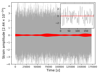
Figure 1: An example of a continuous GW time-domain data, input of TD-Fstat search. Grey time series of $T_{0}$ = 2 sidereal days length mimics the downsampled, narrow-banded data produced from the raw interferometer data [17, 20]. The data contains an almost-monochromatic astrophysical GW signal (red curve) of $\rho_{inj}=10$, and the following parameters (see also Table 1 for the parameters of the search and the text for more details): frequency $f=2.16$ (in the units of the narrow band, between 0 and $\pi$), spindown $\dot{f}=-3.81\times 10^{-8}$ (in dimensionless units of the pipeline, corresponding to $\dot{f}_{astro}=-3.03\times 10^{-9}$ Hz/s; $\dot{f}=\pi\dot{f}_{astro}dt^{2}$ [17]), $\delta=0.474$ (range between $-\pi/2$ and $\pi/2$) and $\alpha=5.84$ (range between 0 and $2\pi$). The reference frequency of the narrow band equals 100 Hz. Visible modulation is the result of the daily movement of the detector with respect to the astrophysical source, as well as of their relative positions, reflecting the quadrupolar nature of the detector’s antenna pattern; in the case of a stationary line local to the detector such modulation is absent.

To generate the candidate signals for the classification, the TD-Fstat search uses narrow-banded time series data as an input. In this work we focus on stationary white Gaussian time series, into which we inject astrophysical-like signals, or monochromatic ‘lines’ imitating local detector’s disturbances. An example of such input data is presented in Fig. 1. It simulates the raw data taken from the detector, downsampled from the original sampling frequency (16384 Hz in LIGO and 20000 Hz in Virgo) to 0.5 Hz, and be divided into narrow frequency bands. Because the frequency of an astrophysical almost-periodic GW signal is not expected to vary substantially (only by the presence of $\dot{f}$), we use a bandwidth of 0.25 Hz, as in recent astrophysical searches [21, 22]. Each narrow frequency band is labeled by a reference frequency, related to the lower edge of the frequency band. Details of the input data are gathered in Table 1. Additional TD-Fstat search input include the ephemeris of the detector (the position of the detector with respect to the Solar System Barycenter and the direction to the source of the signal, for each time of the input data), as well as the pre-defined grid parameter space of ($f$, $\dot{f}$, $\delta$. $\alpha$) values, on which the search ($\mathcal{F}$-statistic evaluations) is performed [24].

In the signal-injection mode, the TD-Fstat search implementation adds an artificial signal to the narrow-band time domain data at some specific $(f,\dot{f},\delta,\alpha)_{inj}$, with an assumed signal-to-noise $\rho_{inj}$. For long-duration almost-monochromatic signals, which are subject of this study, $\rho_{inj}$ is proportional to the length of the time-domain segment $T_{0}$, the amplitude of the signal $h_{0}$ (GW ’strain’) and inversely proportional to the amplitude spectral density of the data $S$, $\rho_{inj}=h_{0}\sqrt{T_{0}/S}$. The output SNR $\rho$ for a candidate signal corresponding to $(f,\dot{f},\delta,\alpha)_{inj}$ is a result of the evaluation of the $\mathcal{F}$-statistic on the Gaussian-noise time series with injected signal. The value of $\rho$ at $(f,\dot{f},\delta,\alpha)_{inj}$ is in general close, but different from $\rho_{inj}$ due to the random character of noise ($\rho$ is related to the value of $\mathcal{F}$-statistic as $\rho=\sqrt{2(\mathcal{F}-2)}$ (see [42] for detailed description). Furthermore it is calculated on a discrete grid. This is the principal reason why we do not study individual signal candidates and their parameters, but the resulting $\rho$ distributions in the $(f,\dot{f},\delta,\alpha)$ parameter space (i.e. at the pre-defined grid of points), since the $\mathcal{F}$-statistic shape is complicated and has several local maxima, as shown e.g. in Fig. 1 of [43]. In the case of pure noise class no additional signal is added to the original Gaussian data, but the data is evaluated in pre-described range of $f,\dot{f},\delta,\alpha$.

Subsequently to produce instances of the three classes for further classification, the code performs a search around the randomly-selected injection parameters $(f,\dot{f},\delta,\alpha)_{inj}$, which in most cases fall in-between the grid points, in the range of a few nearest grid points ($\pm 5$ grid points, see Table 1). In case of cgw all parameters are randomized, whereas for line we take $\dot{f}\equiv 0$. To be consistent in terms of the input data e.g. number of candidate signals, in the case of a stationary line, we also select a random sky position and perform a search in a range similar to the cgw case (this reflects a fact that spectral artifacts may also appear as clusters of candidate signal points in the sky). All the candidate signals crossing the pre-defined $\mathcal{F}$-statistic threshold (corresponding to the SNR $\rho$ threshold) are recorded.

For each configuration of injected SNR $\rho_{inj}$ and reference frequency of the narrow frequency band, we have produced 2500 signals per class (292500 in total). For the cgw class we assumed the simplest distribution over $\rho_{inj}$, i.e. a uniform distribution, as the actual SNR distribution of astrophysical signals is currently unknown. We apply the same ‘agnostic’ procedure for the line class; their real distribution is difficult to define without a detailed analysis of weak lines in the detector data (our methodology allows in principle to include such a realistic SNR distribution in the training set). To train the CNN, we put the lower limit of 8 on $\rho_{inj}$. Above this value, the peaks in the candidate signals $\rho$ distributions for the cgw and line classes are still visible on the $\rho(f,\dot{f},\delta,\alpha)$ plots (see Fig. 2 for the $\rho_{inj}=10$ case). For $\rho_{inj}<8$, the noise dominates the distributions hindering the satisfactory identification of signal classes. Nevertheless, in the testing stage of the algorithm we extend the range of $\rho_{inj}$ down to 4.

To summarize, each instance of the training classes is a result of the following input parameters: $(f,\dot{f},\delta,\alpha)_{inj}$ and $\rho_{inj}$, and consist of a resulting distribution of the candidate signals: values of the SNR $\rho$ evaluations of the TD-Fstat search at the grid points of the frequency $f$ (in fiducial units of the narrow-band, from 0 to $\pi$), spindown $\dot{f}$ (in Hz/s), and two angles describing its sky position in equatorial coordinates, right ascension $\alpha$ (values from 0 to $2\pi$) and declination $\delta$ (values from $-\pi/2$ to $\pi/2$); see Fig. 2 for an exemplary output distribution of the candidate signals.

Detector	LIGO Hanford
Reference band frequency	50, 100, 200, 300, 500, 1000 Hz
	(20, 250, 400, 700, 900 Hz for tests)
Segment length $T_{0}$	2 days
Bandwidth	0.25 Hz
Sampling time $dt$	2 s
Grid range	${\pm}5$ points
$\mathcal{F}$-statistic (SNR) threshold	14.5 (corresponding to $\rho=5$)
Injected signal-to-noise $\rho_{inj}$	from 8 to 20
	(from 4 to 20 for tests)

Table 1: Parameters of the input to the TD-Fstat search code (see e.g., [20]). Time series consist initially of random instances of white Gaussian noise, to which cgws or lines were added. Segment length $T_{0}$ equal to 2 sidereal days with 2 s sampling time results in 86164 data points. The $\mathcal{F}$-statistic (SNR) threshold is applied in order to select signal candidates above certain SNR ratio, to exclude those that are most likely a result of random noise fluctuations.

Figure 2: Exemplary TD-Fstat search outputs for continuous GW signal and stationary line generated for the $\rho_{inj}=10$ and the reference band frequency $f=100$ Hz and parameters of the injected signal from Fig. 1 ($f=2.16$, $\dot{f}=-3.81\times 10^{-8}$, $\delta=0.474$ and $\alpha=5.84$) marked by red vertical lines in the above plots. The left column corresponds to the cgw whereas right column to the line. The distributions represent the relation between recovered SNR $\rho$ ($\mathcal{F}$-statistic SNR) with respect to: the frequency – $a$, the derivative of frequency – $b$, the declination – $c$ and the right ascension – $d$.

The CNN required the input matrix of the fixed size. However, the number of points on distributions shown in Fig. 2 may vary for each simulation. Depending on the frequency (see Table 1) it may increase a few times. To address this issue, we transformed point-based distributions into two different representations: set of four 2D images (four distributions) and set of five 1D vectors (five $\mathcal{F}$-statistic parameters).

The image-based representation was created via conversion to the two-dimensional histogram (see Fig. 3) of the corresponding point-based distributions. Their sizes are $64\times 64$ pixels. We chose this value empirically; smaller images lost some information after the transformation, whereas bigger images led to the significantly extended training time of the CNN we used.

The vector-based representation was created through the selection of the $50$ greatest values of the $\rho$ distribution and their corresponding values from the other parameters ($f$, $\dot{f}$, $\delta$ and $\alpha$). The length of the vector was chosen empirically. The main limitation was related to the density of the point-like distributions which changed proportionally to the frequency. For the 50 Hz signal candidates, the noise class had sparse distributions of slightly more than 50 points. Furthermore, the vectors were sorted with respect to the $\rho$ values, see Fig. 4: this step allowed to reach slightly higher values of classification accuracy.

Figure 3: The 2D representation of TD-Fstat search outputs used as an input to the 2D CNN. Images presented here have same size equal to 64x64 pixels. They correspond to the distributions shown on the left column of Fig. 2: $a$ – (frequency, $\rho$), $b$ – (spindown, $\rho$), $c$ – (declination, $\rho$), $d$ – (right ascension, $\rho$). The colours correspond to the density of the distribution – the brighter it is, the more points contributed to the pixel.

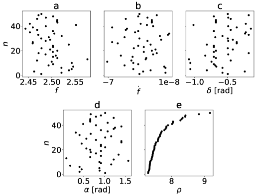
Figure 4: The 1D representation of TD-Fstat search outputs used as an input to the 1D CNN. The outputs are limited to the 50 maximum values of $\rho$ (plots presented here correspond to the distributions shown on the left column of Fig. 2$a$): $a$ – frequency, $b$ – spindown, $c$ – declination, $d$ – right ascension and $e$ – SNR $\rho$. The vector of $\rho$ was sorted since it allowed to reach higher accuracy during training.

The created datasets were then split into three separate subsets: training set (60% of signals from the total dataset), validation set (20% of signals from the total dataset) and the testing set (20% of signals from the total dataset). Validation part was used during training to monitor the performance of the network (whether it overfits). Testing data was used after training to check how the CNN performs with unknown samples.

3.2 Neural network architecture

The generated datasets required two different implementations of the CNN. Overall we tested more than 50 architectures ranging $2-6$ convolutional layers and $1-4$ fully connected layers for both models. Final layouts are shown in Figs. 5$a$ and 5$b$. The architectures which were finally chosen are based on the compromise between the model accuracy and the training time. Models larger than those specified in Fig. 5$a$ and 5$b$ achieved similar performance, but at the cost of significantly longer training time.

In case of 1D CNN, the classifier containing three convolutional layers and two fully connected layers yielded the highest accuracy (more than 94% for the whole validation/test datasets). Whereas the 2D CNN required four convolutional layers and two fully connected layers to reach the highest accuracy (85% over the whole validation/test datasets). The models were trained for 150 epochs which took 1 hour for 1D CNN and 15 hours for 2D CNN (on the same machine equipped with the Tesla K40 NVidia GPU).

To avoid overfitting we included dropout [44] in the architecture of both models. The final set of hyperparameters used for the training was the following for both implementations (definitions of all parameters specified here can be found in [26]): ReLU as the activation function for hidden layers, softmax as the activation function for output later, cross-entropy loss function, ADAM optimizer [45], batch size of 128, and 0.001 learning rate (see Fig. 5$a$ and 5$b$ for other details). The total number of parameters used in our models were the following: 52503 for the 1D CNN, and 398083 for the 2D CNN.

Figure 5: Diagrams show the networks’ layer structure and architecture.

The CNN architectures were implemented using the Python Keras library [46] on top of the Tensorflow library [47], with support for the GPU. We developed the model on NVidia Quadro P6000 and performed the production runs on the Cyfronet Prometheus cluster equipped with Tesla K40 GPUs, running CUDA 10.0 [48] and the cuDNN 7.3.0 [49].

4 Results and discussion

Both CNNs described in Section 3.2, Fig. 5$a$ and Fig. 5$b$ were trained on the generated datasets. During the training model implementing 1D architecture was able to correctly classify 94% of all candidate signals, whereas the model implementing 2D architecture reached 85% of accuracy (see the comparison between learning curves in Fig. 6). Accuracy is defined as the fraction of correctly predicted instances of data to total number of signal candidates. Since the very first epoch, the first model showed better ability to generalize candidate signals over large range of frequencies and values of injected SNR $\rho_{inj}$.

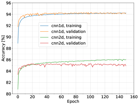
Figure 6: The evolution of the accuracy as a function of the training epoch for the three-label classification for the 1D CNN (upper curves) and 2D CNN (lower curves). Both models reached the maximum accuracy after 40 epochs (based on the results on the validation set). We prolonged training to 150 epochs to investigate the onset of overfitting. The 1D CNN was still properly learning (although without increase of validation accuracy), whereas the 2D CNN showed overfitting - validation accuracy (red curve) maintained at the constant level when training accuracy (green curve) was increasing.

To justify the choice of CNN as an algorithm suitable for the classification of signal candidates, we made a comparison test with different ML methods such as logistic regression, support vector machine (SVM) and random forest. For the test we modified the multi-label classification problem into binary case to create Receiver-Operating-Characteristic (ROC) curves. Classes of line and noise were combined into a single non-astrophysical class. The results of the comparison are shown on Figs. 7$a$ and 7$b$. The results shown on the left figure are corresponding to models trained and tested on 1D data representation, whereas the results shown on the right plot refer to 2D data representation. In both cases the CNNs outperformed other ML models. To further underline the differences, Tab. 2 shows the detection probability (True Positive Rate, TPR) at a $1\%$ of false alarm rate (False Positive Rate or FPR).

Figure 7: The Receiver-Operating-Characteristic (ROC) curves for compared ML algorithms trained on 1D data representation ($a$) and 2D data representation ($b$). The presented results are for the binary classification problem in which $Positive$ stands for cgw whereas $Negative$ corresponds to combined line and noise class. Black dashed line in the middle correspond to random guessing (AUC stands for the Area Under Curve).

CNNs achieved similar level of detection probability significantly outperforming the other algorithms. In case of binary classification or detection of cgw 2D CNN seemed to be slightly better even with much lower accuracy as shown on Fig. 6. However the aim of our work was not only to classify GWs, but also to investigate it’s usefulness on the detection of the stationary line artifacts. The data collected by the GW detectors is noise dominated and polluted by spectral artifacts in various frequency bands, which significantly impact the overall quality of data. Since the CNNs may potentially help in classification of lines to remove them from the science data, the analysis with respect to the multi-label problem is beneficial.

Detection probability of cgw at 1% false alarm rate
	Logistic regression	SVM	Random Forest	CNN
1D data	$33.8$	$31.9$	$89.2$	$96.3$
2D data	$72.8$	$57.6$	$38.4$	$96.8$

Table 2: The summary of detection probabilities for cgw at 1% false alarm rate for compared ML algorithms trained and tested on 1D and 2D data representations.

To decide which CNN architecture was more suitable to the multi-classification, our models were tested against unknown before samples (test dataset), after the training. The results were shown in Fig. 8 in the form of confusion matrix. Both models were able to correctly classify majority of cgw (95.1% for the 1D model and 96.7% for 2D model) as well as the noise (91.3% and 95.7% respectively). However the difference in the classification of the line was significant. 1D CNN was able to correctly classify 96.4% of line candidates whereas 2D CNN only 63.5%. Although the 2D model seemed to be more suited for binary classification task (detection of GW signal from the noise), the 1D CNN outperformed 2D version in the multi-label classification.

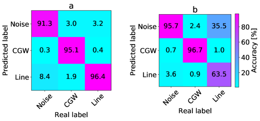
Figure 8: Confusion matrix for the three-label classification evaluated on the test set for the 1D CNN – $a$ and 2D CNN – $b$ after the training. Although the cgw and the noise were classified on the similar level, the line caused significant problem for the 2D model. Majority of line instances resembled noise class in the image representation.

Knowing the general capabilities of designed CNNs, we performed additional tests trying to understand the response of our models against signal candidates of the specific parametrization. We generated additional datasets for particular values of the SNR $\rho_{inj}$ and the frequency (see Table 1). We expanded the $\rho$ range down to value of 4 which corresponds to the $\mathcal{F}$-statistic threshold for the signal candidate. This step allowed us to test the response of the CNN against unknown during training very weak signals that seemed to be indistinguishable from the noise.

The results were presented in Figs. 9$a$ and 9$b$ (for 1D and 2D CNNs, respectively). The 1D model presented significantly more stable behaviour toward the candidates over whole range of considered frequencies. It also maintained nearly stable accuracy for the data with the injected SNR $\rho_{inj}{\geq}10$ (reaching the value of more than 90% for all of them). Interestingly, candidates with $\rho_{inj}<8$ were correctly classified in $60-70$% of samples for frequency $\geq$ 200 Hz. This was relatively high value, taking into consideration their noise-like pattern (for cgw and line instances). This pattern had the biggest influence on the classification of the signal candidates generated for frequencies: 50, 100 Hz and the $\rho_{inj}<8$. The small number of points contributing to the peak (see Fig. 2$a$ for comparison) with respect to the background noise, made these candidates hardly distinguishable from the noise class.

On the other hand, 2D CNN varied significantly in relation to the frequency. It reached the highest accuracy for the 100 Hz (99% for the $\rho_{inj}>10$). For the other frequencies, the maximum accuracy was gradually shifted toward increasing $\rho_{inj}$. Interestingly, the accuracy for the 50 Hz reached the maximum for the $\rho_{inj}=10$; then it gradually decreased. The 2D CNN seemed to outperform 1D model only for the narrow band of the frequency. Nevertheless, the general performance of this implementation was much worse.

Figure 9: The evolution of accuracy as the function of the injected SNR $\rho_{inj}$ for 1D CNN ($a$) and 2D CNN ($b$). The first model achieved maximum level of accuracy for $\rho_{inj}=10-12$ and maintained its value for whole range of frequencies. The 2D version varied significantly in relation to the frequency with the maximum accuracy being gradually shifted toward larger values of $\rho_{inj}$. Characteristic shift in the accuracy (upper plot) between the lower frequencies (50 and 100 Hz) and the rest was associated with the density of signal candidates distributions. cgw and line instances were easier to separate from noise since their distributions of parameters had very sparse character (see Fig 2 for comparison) - the noise signal candidates were not grouping around fluctuations in the frequency domain (the background of Fig. 2$a$) allowing easier classification than for higher frequencies.

Since the 1D CNN proved to be more accurate over broad range of frequencies, we chose it as a more useful model in the classification of the $\mathcal{F}$-statistic signal candidates. Below we present the results of additional tests we performed to better understand its usability.

To tests the model response toward particular signal candidate, we computed sensitivity (in ML literature also referred as the recall) defined as the fraction of relevant instances among the retrieved instances. Figure 10 presents the results. Classification of the cgw was directly proportional to the $\rho_{inj}$ up to value of 11-12, then the sensitivity saturated around 95%-99% depending on the frequency. For $\rho_{inj}$ approaching 4, sensitivity decreased to 0%. This result was expected since the injected signal at this level is buried so deeply in the noise that is indistinguishable. Furthermore by comparing Fig. 10 $a$ with Fig. 9 $a$, we deduced that the classification of cgw had the biggest influence on the total performance of the CNN.

The sensitivity of the line for higher frequencies (more than 300 Hz) maintained at relatively constant level of more than 95% even for the smallest $\rho_{inj}$. Decrease in sensitivity for lower frequencies was associated with the density of the signal candidates distribution. The outputs of TD-Fstat had the more sparse character, the lower frequency was. Chosen 50 points for the input data were taken not only from the peak but also from the background noise (see top plots from Fig. 2). With decreasing $\rho_{inj}$ background points started to dominate and the candidates seemed to resemble noise class. This leads to misclassification of nearly all line samples for 50 Hz data.

In case of the noise, sensitivity was inversely proportional to the frequency. Again this was associated with the density of the signal candidates distributions. For higher frequencies more points contributed to local fluctuations. As a result the 50 points chosen for the input data, instead of having random character, resembled different types of candidates.

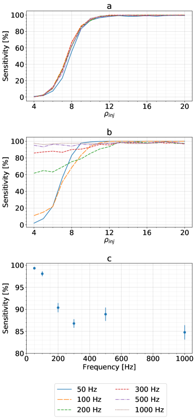
Figure 10: The evolution of sensitivity as a function of SNR $\rho_{inj}$ of the 1D CNN for the three types of signal candidates: cgw – $a$, line – $b$, and noise – panel $c$. The last panel shows average values for frequencies, because the noise classification sensitivity is not a function of the injected SNR $\rho_{inj}$, and stays approximately constant for each narrow-band frequency value.

We additionally performed tests on the signal candidates generated for different frequencies than specified in the Table 1. We chose five new frequencies to test the model on: 20, 250, 400, 700, 900 Hz. The results were presented in Fig. 11. The 20 Hz case is missing since the number of available points (from initial distributions) to create set of five 1D vectors was much smaller than the chosen length (some distributions for the noise class contained less than 10 points). Nevertheless, the CNN for the other frequencies reached similar accuracies as those presented in Fig. 9$a$. This result proved the generalization ability of the 1D CNN toward unknown frequencies. However the limitation of the model was the minimum number of candidate signals available to create input data. Since this number was proportional to the number of grid points (frequency) of the searched signal, our CNN was not suited to search for candidates below 50 Hz.

Figure 11: The evolution of accuracy as the function of the injected SNR $\rho_{inj}$ for 1D CNN for the signal candidates generated with frequencies different from those used for the training.

Although it is not immediately apparent from the 1D and 2D instances of the distributions of candidate signals, the $\mathcal{F}$-statistic values in the sky points contain non-negligible information about the signal content, and play a role in increasing the classification accuracy. A dedicated study of the influence of the distribution of the $\mathcal{F}$-statistic in the sky for astrophysical signals and detector artifacts will be addressed in a separate study.

5 Conclusions

We proved that the CNN can be successfully applied in the classification of TD-Fstat search results, multidimensional vector distributions corresponding to three signal types: the GW signal, the stationary line and the noise. We compared 2D and 1D implementations of CNN. The latter achieved much higher accuracy (94% with respect to 85%) over candidate signals generated for broad range of frequencies and $\rho_{inj}$. For majority of signals ($\rho_{inj}{\geq}10$) 1D CNN maintained more than 90% of accuracy. This level of accuracy was preserved at the classification of the signal candidates injected in bands of unknown frequency (i.e. we show that the constructed CNNs are able to generalize the context).

2D CNN represented a different character. Although, the overall accuracy was worse than 1D model, the 2D version seemed to achieve better results as a binary classifier (between the cgw and the noise). Representation of the input data in the form of the image seemed to cause significant problems for the proper classification of the line. Even though the 2D CNN had worse generalization ability, it was able to outperform the 1D implementation for the narrow-band frequencies 100 Hz and below. Nevertheless, 1D CNN with its ability to generalize unknown samples (in particular with respect to the frequency) seemed to be better choice for the realistic applications.

This project, as one of the few, researches the application of DL as a supplementary component to MF. Adopting signal candidates as the DL input instead of raw data allows to avoid problems that other researchers encountered. This approach limits the number of signals to those that exceeded the $\mathcal{F}$-statistic threshold, i.e. analysed distribution instances are firmly characterized by known significance. As Gebhard et al. [31]) described, application of DL on raw data provides signal candidates of unknown or hard to define significance. Before DL could be used as a safe alternative to MF for the detection of GW, it has to be studied further. However, our results can already be considered in terms of supporting role to MF. For example, it could be applied to the pre-processing of signal candidates for the further steps follow-up via fast classification, and to limit the parameter space to be processed further. As our results shows, a relatively simple CNN can also be used in the classification of spectral artifacts e. g., as an additional tool for flagging and possibly also removing spurious features from the data. Among the many possibilities for further development within the are of CW searches we are considering is also the application of DL in the follow-up of signal candidates in multiple data segments (post-processing searches for patterns), as well as the analysis of data from the network of detectors.

Data Availability Statement

The data that support the findings of this study are available from the corresponding author upon reasonable request.

References

References

- [1] Einstein A 1916 Sitzungsberichte der Königlich Preußischen Akademie der Wissenschaften (Berlin), Seite 688-696.
- [2] Aasi J, Abbott B P, Abbott R, Abbott T et al. 2015 \cqg 32 074001 (Preprint 1411.4547)
- [3] Acernese F, Agathos M, Agatsuma K, Aisa D et al. 2015 \cqg 32 024001 (Preprint 1408.3978)
- [4] Abbott B P, Abbott R, Abbott T D, Abernathy M R, Acernese F, Ackley K, Adams C, Adams T, Addesso P, Adhikari R X and et al 2016 Physical Review Letters 116 061102 (Preprint 1602.03837)
- [5] Abbott B P, Abbott R, Abbott T D, Acernese F, Ackley K, Adams C, Adams T, Addesso P, Adhikari R X, Adya V B and et al 2017 Physical Review Letters 118 221101 (Preprint 1706.01812)
- [6] Abbott B P, Abbott R, Abbott T D, Acernese F, Ackley K, Adams C, Adams T, Addesso P, Adhikari R X, Adya V B and et al 2017 Physical Review Letters 119 141101 (Preprint 1709.09660)
- [7] Abbott B P, Abbott R, Abbott T D, Acernese F, Ackley K, Adams C, Adams T, Addesso P, Adhikari R X, Adya V B and et al 2017 Physical Review Letters 119 161101 (Preprint 1710.05832)
- [8] The LIGO Scientific Collaboration, the Virgo Collaboration, Abbott B P, Abbott R, Abbott T D, Abraham S, Acernese F, Ackley K, Adams C, Adhikari R X and et al 2018 arXiv e-prints (Preprint %****␣main.bbl␣Line␣50␣****1811.12907)
- [9] Lasky P D 2015 Publications of the Astronomical Society of Australia 32
- [10] Sieniawska M and Bejger M 2019 Universe 5 217 (Preprint 1909.12600)
- [11] Abbott B P, Abbott R, Abbott T D, Abernathy M R, Acernese F, Ackley K, Adams C, Adams T, Addesso P, Adhikari R X and et al 2017 ApJ 839 12 (Preprint 1701.07709)
- [12] Abbott B P, Abbott R, Abbott T D, Acernese F, Ackley K, Adams C, Adams T, Addesso P, Adhikari R X, Adya V B and et al 2017 Phys. Rev. D 96 122006 (Preprint 1710.02327)
- [13] Abbott B P, Abbott R, Abbott T D, Acernese F, Ackley K, Adams C, Adams T, Addesso P, Adhikari R X, Adya V B and et al 2017 Phys. Rev. D 96 062002 (Preprint 1707.02667)
- [14] Abbott B P, Abbott R, Abbott T D, Acernese F, Ackley K, Adams C, Adams T, Addesso P, Adhikari R X, Adya V B and et al 2018 Phys. Rev. D 97 102003 (Preprint 1802.05241)
- [15] Bejger M 2017 Rencontres de Moriond (Preprint 1710.06607)
- [16] Jaranowski P, Królak A and Schutz B F 1998 Phys. Rev. D 58(6) 063001
- [17] Astone P, Borkowski K M, Jaranowski P, Pietka M and Królak A 2010 Phys. Rev. D 82 022005 (Preprint arXiv:1003.0844)
- [18] Time-domain -statistic pipeline repository https://github.com/mbejger/polgraw-allsky accessed: 2018-09-04
- [19] Time-domain -statistic pipeline documentation http://mbejger.github.io/polgraw-allsky accessed: 2018-09-04
- [20] Aasi J, Abbott B P, Abbott R, Abbott T, Abernathy M R, Accadia T, Acernese F, Ackley K, Adams C, Adams T and et al 2014 Classical and Quantum Gravity 31 165014 (Preprint arXiv:1402.4974)
- [21] Abbott B P, Abbott R, Abbott T D, Acernese F, Ackley K, Adams C, Adams T, Addesso P, Adhikari R X, Adya V B and et al 2017 Phys. Rev. D 96 122004 (Preprint 1707.02669)
- [22] Abbott B P, Abbott R, Abbott T D, Abraham S, Acernese F, Ackley K, Adams C, Adhikari R X and et al 2019 arXiv e-prints arXiv:1903.01901 (Preprint 1903.01901)
- [23] Walsh S, Pitkin M, Oliver M, D’Antonio S, Dergachev V, Królak A, Astone P, Bejger M, Di Giovanni M and Dorosh O 2016 Phys. Rev. D 94 124010 (Preprint 1606.00660)
- [24] Pisarski A and Jaranowski P 2015 Classical and Quantum Gravity 32 145014 (Preprint arXiv:1302.0509)
- [25] Poghosyan G, Matta S, Streit A, Bejger M and Królak A 2015 Computer Physics Communications 188 167–176 ISSN 0010-4655 URL http://dx.doi.org/10.1016/j.cpc.2014.10.025
- [26] Goodfellow I, Bengio Y and Courville A 2016 Deep Learning (The MIT Press) ISBN 0262035618, 9780262035613
- [27] Razzano M and Cuoco E 2018 Class. Quant. Grav. 35 095016 (Preprint 1803.09933)
- [28] Beheshtipour B and Papa M A 2020 Phys. Rev. D 101 064009 (Preprint 2001.03116)
- [29] George D and Huerta E A 2018 Physics Letters B 778 64–70 (Preprint 1711.03121)
- [30] Dreissigacker C, Sharma R, Messenger C and Prix R 2019 arXiv e-prints arXiv:1904.13291 (Preprint 1904.13291)
- [31] Gebhard T D, Kilbertus N, Harry I and Schölkopf B 2019 arXiv e-prints arXiv:1904.08693 (Preprint 1904.08693)
- [32] Lecun Y, Bengio Y and Hinton G 2015 Nature 521 436–444
- [33] Samuel A L 1959 IBM J. Res. Dev. 3 210–229 ISSN 0018-8646 URL http://dx.doi.org/10.1147/rd.33.0210
- [34] Maronidis A, Chatzilari E, Nikolopoulos S and Kompatsiaris I 2018 Digital Signal Processing 74 14–29
- [35] Druzhkov P N and Kustikova V D 2016 Pattern Recognition and Image Analysis 26 9–15 ISSN 1555-6212 URL https://doi.org/10.1134/S1054661816010065
- [36] Zhang Z, Geiger J, Pohjalainen J, Mousa A E D, Jin W and Schuller B 2018 ACM Trans. Intell. Syst. Technol. 9 49:1–49:28 ISSN 2157-6904 URL http://doi.acm.org/10.1145/3178115
- [37] Collobert R, Weston J, Bottou L, Karlen M, Kavukcuoglu K and Kuksa P 2011 J. Mach. Learn. Res. 12 2493–2537 ISSN 1532-4435 URL http://dl.acm.org/citation.cfm?id=1953048.2078186
- [38] Lukic V and Brüggen M 2016 Proceedings of the International Astronomical Union 12 217–220
- [39] Hon M, Stello D and Yu J 2017 Royal Astronomical Society. Monthly Notices 469 4578–4583 ISSN 0035-8711
- [40] Research B 2018 (accessed February 9, 2018) DeepBench URL https://github.com/baidu-research/DeepBench
- [41] Covas P B, Effler A, Goetz E, Meyers P M, Neunzert A, Oliver M, Pearlstone B L, Roma V J, Schofield R M S, Adya V B and et al 2018 Phys. Rev. D 97 082002 (Preprint 1801.07204)
- [42] Jaranowski P and Krolak A 2009 Analysis of Gravitational-Wave Data (Cambridge, UK: Cambridge University Press)
- [43] Sieniawska M, Bejger M and Królak A 2019 Classical and Quantum Gravity 36 225008 ISSN 1361-6382 URL http://dx.doi.org/10.1088/1361-6382/ab3ee5
- [44] Srivastava N, Hinton G, Krizhevsky A, Sutskever I and Salakhutdinov R 2014 Journal of Machine Learning Research 15 1929–1958 URL http://jmlr.org/papers/v15/srivastava14a.html
- [45] Kingma D P and Ba J 2014 arXiv e-prints arXiv:1412.6980 (Preprint 1412.6980)
- [46] Chollet F et al. 2015 Keras https://keras.io
- [47] Abadi M, Agarwal A, Barham P, Brevdo E, Chen Z, Citro C, Corrado G S, Davis A, Dean J, Devin M, Ghemawat S, Goodfellow I, Harp A, Irving G, Isard M, Jia Y, Jozefowicz R, Kaiser L, Kudlur M, Levenberg J, Mané D, Monga R, Moore S, Murray D, Olah C, Schuster M, Shlens J, Steiner B, Sutskever I, Talwar K, Tucker P, Vanhoucke V, Vasudevan V, Viégas F, Vinyals O, Warden P, Wattenberg M, Wicke M, Yu Y and Zheng X 2015 TensorFlow: Large-scale machine learning on heterogeneous systems software available from tensorflow.org URL https://www.tensorflow.org/
- [48] Nickolls J, Buck I, Garland M and Skadron K 2008 Queue 6 40–53 ISSN 1542-7730 URL http://doi.acm.org/10.1145/1365490.1365500
- [49] Chetlur S, Woolley C, Vandermersch P, Cohen J, Tran J, Catanzaro B and Shelhamer E 2014 ArXiv e-prints (Preprint 1410.0759)