Persistent homology analysis of multiqubit entanglement

Abstract

We introduce a homology-based technique for the analysis of multiqubit state vectors. In our approach, we associate state vectors to data sets by introducing a metric-like measure in terms of bipartite entanglement, and investigate the persistence of homologies at different scales. This leads to a novel classification of multiqubit entanglement. The relative occurrence frequency of various classes of entangled states is also shown.

I Introduction

Entanglement has been recognized as a key resource for obtaining a quantum boost in many information technology tasks (see e.g. WGE16 ). As such it deserves a careful characterization. Initial work on the classification of entangled states was focussed on the quantification through so-called ‘entanglement monotones’, i.e. functions of multipartite states that do not increase under local transformations vidal . These functions have been proved to work well mostly for bipartite states Horo , while for multipartite entanglement another approach seems to be more promising, which is based on partitioning states according to some notion of equivalence. In the SLOCC approach dur , equivalence classes are constructed on the base of invariance under stochastic local operations and classical communication. However, this leads to infinite (even uncountable) classes for more than three qubit systems. Hence this approach is not effective in the general case, although some ways out were devised for the case of four qubits four .

An alternative route to entanglement classification is represented by the analysis of topological features of multipartite quantum states Quinta ; PH1 . Topological data analysis has recently gained a lot of attention in the classical framework thanks to its suitability for the analysis of huge data sets represented in the form of point clouds: in such cases, it would indeed be impossible to accurately analyze the data, while a “qualitative" analysis would be efficient. Among these techniques, Persistent Homologies (PH) played a pivotal role Edel ; Carl . It is a particular sampling-based technique from algebraic topology aiming at extracting topological information from high-dimensional data sets.

Here, following up the work in PH1 , we apply PH techniques to analyse multiqubit state vectors. Each state vector will be intended as a data set by introducing a metric-like measure in terms of bipartite entanglement. Then the persistence of homologies at different scales will be investigated. While the aim of PH1 was the classification of all possible states for 3 and 4 qubit, here we focus on ‘genuine entanglement’ and show the classification up to 6 qubit. Moreover, in this paper we will also compute the relative occurrence frequency of the various classes of entangled states, by means of a random generation of states.

The article is organized as follow. In Section II we briefly recall concepts of algebraic topology that will be used thereafter. In Section III we illustrate the method to produce a data cloud from multiqubit states. Then we produce and show the barcodes for the cases of 4 and 5 qubit in Section IV (those for 6 qubit are reported in the Appendix). There we also analyze the occurrence frequency of various classes of entangled states. Finally, we draw our conclusions in Section V.

II Persistent Homology

A data cloud is a collection of points in some $n$-dimensional space $\mathbb{S}_{n}$. In many cases, analysing the global ’shape’ of the point cloud gives essential insights about the problem it represents. In the context of data analysis, Persistent Homology is an algebraic method for computing coarse topological features of a given data cloud that persist over many grouping scales. In this section we review the mathematical background that is necessary to understand this technique Hatcher ; Edelsbrunner .

Consider a data cloud represented by a set of points $\left\{x_{\alpha}\right\}$ living in a Euclidean space. Choosing a value of the grouping scale $\epsilon$, it is possible to construct the graph whose vertices are the data points $\left\{{x_{\alpha}}\right\}$ and edges $e_{x_{\alpha},x_{\alpha^{\prime}}}$ are drawn when the $\frac{\epsilon}{2}$-balls centered in the vertices ${x_{\alpha}}$ and $x_{\alpha^{\prime}}$ intersect each other. Such graphs show connected components and hence clusters obtained at $\epsilon$ scale but do not provide information about higher-order features such as holes and voids. In order to track high-dimensional features we need to introduce the following concepts.

Convex set. A convex set is a region of a Euclidean space where every two points are connected by a straight line segment that is also within the region.

Convex Hull. The convex hull of a set $X$ of points in an Euclidean space is the smallest convex set that contains $X$.

$k$-Simplex. A $k$-simplex is a $k$-dimensional polytope which is the convex hull of its $k+1$ vertices. Thus, for example, simplices of dimension $0,1,2$ and $3$ are respectively vertices, edges, triangles and tetrahedra.

Simplicial Complex. A simplicial complex ${\mathcal{K}}$ is a set of simplices that satisfies the conditions:

1. Any face of a simplex from ${\mathcal{K}}$ is also in ${\mathcal{K}}$.

2. The intersection of any two simplices $\sigma_{1},\sigma_{2}\in{\mathcal{K}}$ is either the empty set $\emptyset$ or a face of both $\sigma_{1}$ and $\sigma_{2}$.

The dimension of a simplicial complex is equal to the largest dimension of its simplices.

Homology of a complex.

For each simplicial complex ${\mathcal{K}}$ there is a set of homological groups $\left\{H_{0}({\mathcal{K}}),H_{1}({\mathcal{K}}),H_{2}({\mathcal{K}}),\ldots\right\}$, where the $k$th homology group $H_{k}({\mathcal{K}})$ is non-empty when the $k$-dimensional holes are in ${\mathcal{K}}$. Hence, the homological groups of the simplicial complex describe the order of the holes existing in that simplicial complex.

In order to recognize global topological features of a data cloud it is necessary to complete the corresponding graph to a simplicial complex by filling in the graph with all the simplices. Given a grouping scale $\epsilon$, there are different methods to generate simplicial complexes. In this paper we will focus on the Rips complex, $\mathcal{R}_{\epsilon}$, where $k$-simplices correspond to $(k+1)$ points which are pairwise within distance $\epsilon$.

Topological features of the data cloud are obtained by constructing a homology of the simplicial complex. The homology of the Rips complex hence reveal those topological features that appear at a chosen value of $\epsilon$. If $\epsilon$ is taken too small, then only multiple connected components are shown. On the other hand, when $\epsilon$ is large, any pairs of points get connected and a giant simplex with trivial homology is obtained. However, it is preferable to make the whole process independent from the choice of $\epsilon$. In order to obtain significant features it is necessary to consider all the range of $\epsilon$. Those topological features which persist over a significant interval of the parameter $\epsilon$ are to be considered specific of that point cloud, while short-lived features as less important ones. Consider the sequence of Rips complexes $\mathsf{R}=\left\{\mathcal{R}_{\epsilon_{i}}\right\}_{i=1}^{N}$ associated to a given point cloud; instead of examining the homology of the individual terms $H(\mathcal{R}_{\epsilon_{i}})$, we look at the inclusion maps $I:H(\mathcal{R}_{\epsilon_{i}})\rightarrow H(\mathcal{R}_{\epsilon_{j}})$ for all $i<j$. These maps are able to tell us which features persist since they reveal information that is not visible if we consider $H(\mathcal{R}_{\epsilon_{i}})$ and $H(\mathcal{R}_{\epsilon_{j}})$ separately.

Barcodes. Given the sequence of Rips complexes $\mathsf{R}=\left\{\mathcal{R}_{\epsilon_{i}}\right\}_{i=1}^{N}$, a barcode is a graphical representation of $H_{k}(\mathsf{R})$ as a collection of horizontal line segments in a plane whose horizontal axis corresponds to the parameter $\epsilon$ and whose vertical axis represents an (arbitrary) ordering of homology groups. A barcode can be seen as a variation over $\epsilon$ of the Betti numbers which count the number of $n$-dimensional holes on a simplicial complex $\mathcal{R}_{\epsilon}$ (cf. Barcodes ).

III Creating qubit data cloud

In this section we discuss the methodology we use for creating the data cloud which will be at basis of classifying entangled states. We will restrict our attention to $N$ qubit states showing "genuine" entanglement, i.e. that are $N$-partite entangled or “fully inseparable".

Our approach starts with the random generation of pure states among which we select, using generalised concurrence measure, those showing genuine entanglement. At this stage, a data cloud is associated to a state in such a way that each qubit is identified with a single point in the cloud, while a distance between pairs of points is defined using a semi-metric that takes into account the pairwise entanglement shared by the two qubits that the points represent. Semi-distances between qubits are stored in a matrix $D$ which will be the input of the persistent homology algorithm.

Note that in the definitions given in Section II we refer for simplicity to Euclidean spaces. Since here we are dealing instead with a semi-metric space, it is worth stressing that computing persistent homology is still possible in our case. In fact, a distance between pairs of points which does not satisfy triangular inequality is still sufficient for constructing Rips complexes.

III.1 Random state generation

In order to randomly generate a pure state of $N$ qubits, we employ the following parametrization Zyczkowski_2001 ; PhysRevA.94.022341

$$|\psi\rangle=\sum_{n=0}^{2^{N}-1}\nu_{n}|n\rangle,$$ (1)

with

$$\nu_{0} = \cos\theta_{2^{N}-1},$$ (2)

$$\nu_{n>0} = e^{i\phi_{n}}\cos\theta_{2^{N}-1-n}\prod_{l=2^{N}-n}^{2^{N}-1}\sin\theta_{l}.$$ (3)

and

$$\theta_{n}:=\arcsin\left(\xi_{n}^{\frac{1}{2n}}\right).$$ (4)

The independent random variables $\phi_{n\geq 1}$ and $\xi_{n\geq 0}$ are uniformly distributed in the intervals:

$$\phi_{n\geq 1}\in[0,2\pi),\qquad\xi_{n}\in[0,1].$$

III.2 Entangled states selection

After generating a random $N$-qubit state $|\psi\rangle$ we check that it is actually $N$-partite entangled. This happens iff for every bipartition $A/\hat{A}$ (where $\hat{A}$ denotes the complement set of $A$) of the $N$-qubit, ${\cal C}_{G}(\rho_{A})\neq 0$, where ${\cal C}_{G}$ is the generalized concurrence defined in GenConcurrence as follows:

$$\mathcal{C}_{G}(\rho_{A}):=2\sqrt{1-{\rm Tr}(\rho_{A}^{2})}.$$ (5)

III.3 Distances calculation

It is possible to generate barcodes for simplicial complexes corresponding to a points (i.e.qubits) cloud by giving in input to the persistent homology algorithm the matrix $D$ of all pairwise distances between points.
In PH1 , a semi-distance $1/E_{i,j},$ was proposed, where $E_{i,j}$ is an entanglement monotone calculated between qubit $i$ and qubit $j$. This semi-distance goes from 1 (when the two qubit are maximally entangled) to +$\infty$ (when they are separable). Here we use the following semi-metric:

$$D_{i,j}=1-\exp\left\{1-\dfrac{1}{C_{i,j}}\right\},$$ (6)

where $C_{i,j}$ is the concurrence between qubit $i$ and qubit $j$. The semi-distance $D_{i,j}$ goes from $0$ to $1$ as the entanglement decreases, and remains finite for separable states.

Recall that, given a state $\rho$ on $N$ qubits, the concurrence between two qubits $i$ and $j$ is obtained by first tracing out all other $N-2$ qubits. This gives the reduced density matrix $\rho_{ij}$. Then

$$C_{i,j}:=\max\{0,\lambda_{1}-\lambda_{2}-\lambda_{3}-\lambda_{4}\},$$ (7)

where $\lambda_{1},\lambda_{2},\lambda_{3},\lambda_{4}$, are the square root of the eigenvalues (in decreasing order) of the matrix $\rho_{ij}(\sigma_{y}\otimes\sigma_{y})\rho^{*}_{ij}(\sigma_{y}\otimes\sigma_{y})$ Concurrence , with $\sigma_{y}$ the well known Pauli matrix and $\rho^{*}_{ij}$ the complex conjugate of $\rho_{i,j}$ in the computational basis.

IV Entanglement classification

We have used the TDA package for computing persistent homology and barcodes developed for the R software. The classification is obtained grouping together those states with the same barcode.

In the following barcodes, black lines represent connected components (i.e. homology group $H_{0}$), red lines represent holes (i.e. homology group $H_{1}$) and blue lines represent voids (i.e. homology group $H_{2}$). All barcodes are generated using the Rips complex.

IV.1 Classification of four qubits states

Barcodes generated by 4-partite entangled states of 4 qubits and relative frequencies are shown starting from the most frequent to the least frequent one.

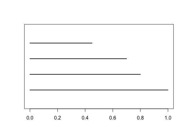
Figure 1: Barcode of the class labelled as 4B1

Genuine entangled states with the barcode shown in Figure 1 have a total of four connected components: three of them end at value of $\epsilon<1$, while only one component persists over all the range of $\epsilon$. The fact that only one connected component persists means that the state form a single cluster of qubits grouped by pairwise entanglement without showing higher homological features. A representative of such class is the $|W\rangle$ state.

$$|4,B1\rangle=|W\rangle=\frac{1}{2}(|0001\rangle+|0010\rangle+|0100\rangle+|1000\rangle)$$

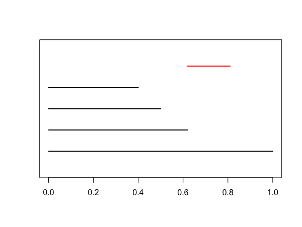
Figure 2: Barcode of the class labelled as 4B2

States belonging to class of Figure 2 form again a single persistent component of pairwise entanglement between qubits. However in this case a hole, denoted by the red bar $H_{1}$, appears when only one connected component is left. Such a hole has limited life-span since disappears when $\epsilon$ is sufficiently large. A state showing such a behaviour is the following:

$$\begin{split}|4,B2\rangle=\dfrac{1}{2\sqrt{2}}\left(\sqrt{2}|0000\rangle+|0011\rangle+|0110\rangle+|1001\rangle+\right.\\ \left.+|1100\rangle+\sqrt{2}|1111\rangle\right)\end{split}$$

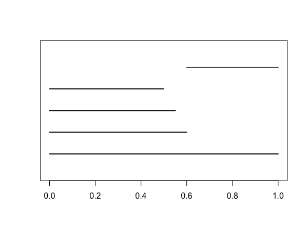
Figure 3: Barcode of the class labelled as 4B3

In the case shown in Figure 3, a single connected component is left and a persistent hole is present. States with this barcode have the characteristic that each qubit is pairwise entangled to other two qubits and completely un-entangled with a third qubit. A state showing such properties is

$$|4,B3\rangle={{\frac{1}{2}}}\left(|0000\rangle+|0011\rangle+|1010\rangle+|1111\rangle\right)$$

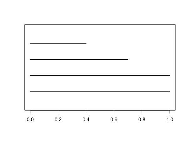
Figure 4: Barcode of the class labelled as 4B4

In the class represented by the barcode in Figure 4 we find genuinely entangled states with no higher homological feature than $H_{0}$ which have two different connected component that persist over the range of $\epsilon$. This means that such states have two sets of qubits which are internally connected by pairwise entanglement to form a component, but no connection is present among qubits of different sets. Yet a single qubit in a set could be entangled to the other set as a whole. An example for this class is the state:

$$|4,B4\rangle=\frac{1}{2}\left(|0011\rangle+|1011\rangle+|1101\rangle+|1110\rangle\right)$$

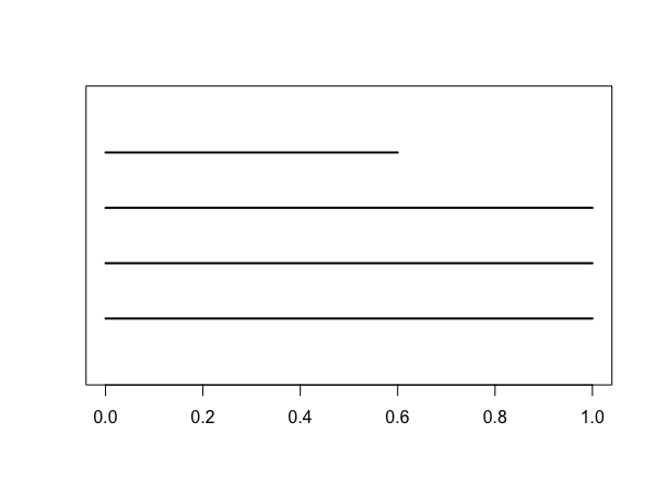
Figure 5: Barcode of the class labelled as 4B5

Like the previous case, states with the barcode of Figure 5 only show four connected components, three of which persist while one has limited lifetime. The characteristic of these states is that there are always 2 qubits which do not share any pairwise entanglement with another qubit, while the other two do. A representative state for this class is

$$|4,B5\rangle=\dfrac{1}{\sqrt{3}}\left(|0000\rangle+|0111\rangle+|1101\rangle\right)$$

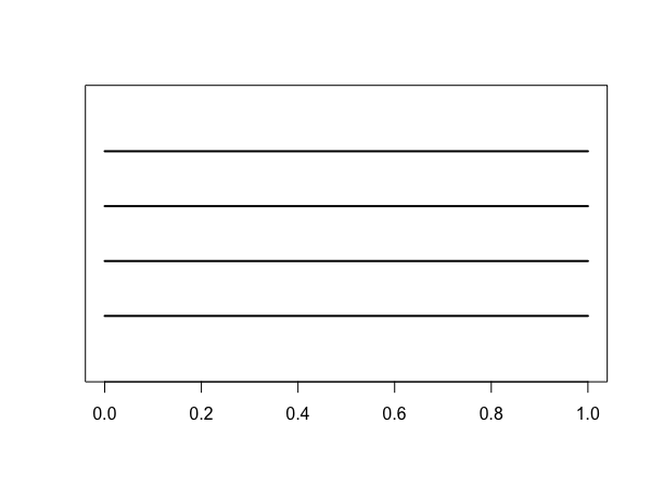
Figure 6: Barcode of the class labelled as 4B6

States of the kind shown in Figure 6 do not have any pairwise entanglement among qubits. For this reason no qubit get connected to another and we see four distinct components that persist. A representative of this class is the $|\text{GHZ}\rangle$ state.

$$|4,B6\rangle=|\text{GHZ}\rangle=\frac{1}{\sqrt{2}}(|0000\rangle+|1111\rangle)$$

As we can observe in Fig.7, there exist six different classes of four qubit genuine entangled states, based on the persistent homology classification. The most frequent class ($61.70\%$) is the one where only one component persists (4B1), states like W belong to to this class. With frequencies of $17.31\%$ and $10.60\%$ we find states with barcodes 4B2 and 4B3 showing one persistent connected component and a hole (red line) that in the case of 4B3 is also persistent. The last three barcodes, in order 4B4, 4B5 and 4B6 show an increasing number of disconnected components. States that are GHZ-like are hence the least frequent ($0.52\%$).

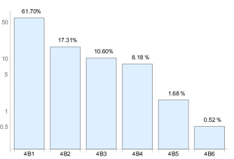
Figure 7: Barcode frequencies (in Log scale) for four qubits genuine entangled states

IV.2 Classification of five qubits states

Let’s now consider randomly generated 5-partite entangled states of 5 qubits. Barcodes and relative frequencies are shown below starting from the barcode more likely to appear to the least frequent one.

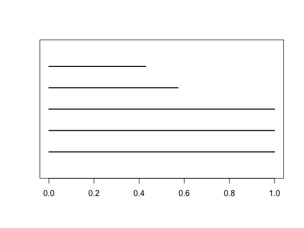
Figure 8: Barcode of the class labelled as 5B1

In the five qubit case, the most frequent class shows a barcode like the one in Figure 8 with three connected components that persist in the range of $D$. States of this kind have at least one qubit (up to two qubits) that does not share pairwise entanglement with any other qubit. This configuration does not generate higher homology groups than $H_{0}$. An example of state in this class is

$$\begin{split}|5,B1\rangle=\dfrac{1}{\sqrt{5}}\left(|00001\rangle+|00011\rangle+\right.\\ \left.+|00110\rangle+|01000\rangle+|11011\rangle\right)\end{split}$$

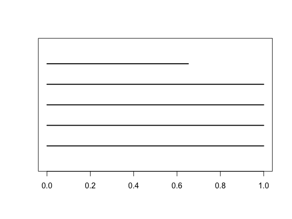
Figure 9: Barcode of the class labelled as 5B2

As we can see, the barcode of Figure 9 shows four persistent connected components i.e. only two qubits among five share pairwise entanglement while all remaining qubits act as independent connected component. A representative state for this class is

$$\begin{split}|5,B2\rangle=\dfrac{1}{\sqrt{5}}\left(|00001\rangle+|00011\rangle+\right.\\ \left.+|00100\rangle+|01100\rangle+|11010\rangle\right)\end{split}$$ (8)

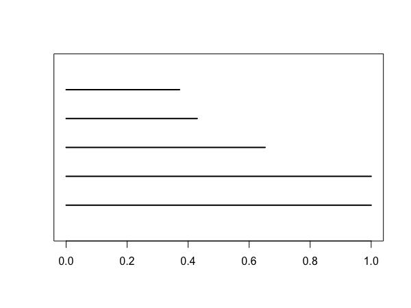
Figure 10: Barcode of the class labelled as 5B3

In this class identified by the barcode of Figure 10, two connected components persist while the other three have limited lifetime. Two clusters of qubits connected by pairwise entanglement are hence created and no holes or higher topological features appear. An example of state in this class is the following

$$\begin{split}|5,B3\rangle=\dfrac{1}{\sqrt{5}}\left(|00001\rangle+|00010\rangle+\right.\\ \left.+|00100\rangle+|01000\rangle+|10111\rangle\right)\end{split}$$

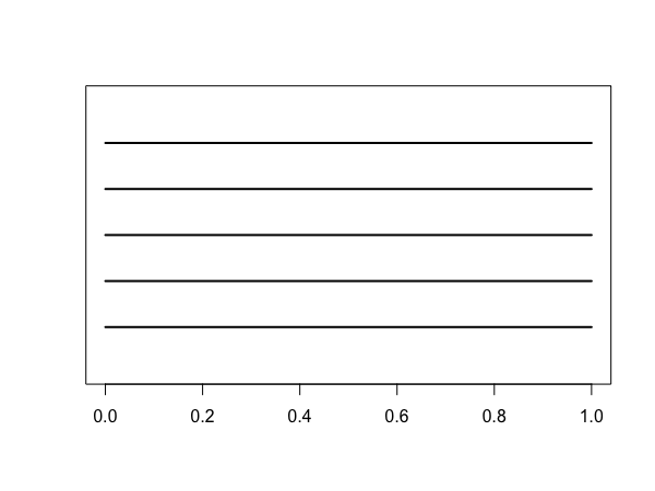
Figure 11: Barcode of the class labelled as 5B4

Figure 11 show the barcode of the class where we find GHZ like states, i.e. those states where there are no entangled pair of qubits and hence show five persistent connected components in the barcode.

$$\begin{split}|5,B4\rangle=\dfrac{1}{\sqrt{2}}\left(|00000\rangle+|11111\rangle\right)\end{split}$$

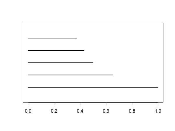
Figure 12: Barcode of the class labelled as 5B5

After we find the barcode shown in Figure 12 and relative to those states like $|W\rangle$ which have only one connected component and hence pairwise entanglement creates a single cluster of qubits.

$$\begin{split}|5,B5\rangle=\dfrac{1}{\sqrt{5}}\left(|00001\rangle+|00010\rangle+\right.\\ \left.+|00100\rangle+|01000\rangle+|10000\rangle\right)\end{split}$$

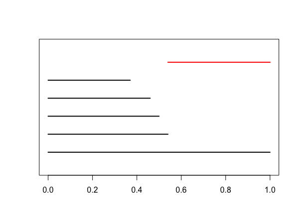
Figure 13: Barcode of the class labelled as 5B6

Figure 13 shows the barcode of the first class of 5 qubits genuinely entangled states that present a first order homology group $H_{1}$, i.e. a hole, in the barcode. States in this class have their qubits connected to form a single persistent component when $\epsilon\approx 1$. Note also that some subsets of qubits do not share any pairwise entanglement and hence are responsible for the persistent hole. An example of state in this class is

$$\begin{split}|5,B6\rangle=\dfrac{1}{\sqrt{6}}\left(|00000\rangle+|11000\rangle+\right.\\ \left.+|01100\rangle+|00110\rangle+|00011\rangle+|10001\rangle\right)\end{split}$$

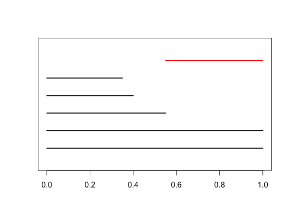
Figure 14: Barcode of the class labelled as 5B7

As we can see in Figure 14, like in the previous class, a hole is created at some value of $\epsilon$ and persists up to the upper limit of the semi-metric $D$. However here while four qubits are responsible for one connected component and for the $H_{1}$ homology, the remaining fifth qubit does not share any pairwise entanglement with the others and creates a persistent component on its own. A representative state of this kind is

$$\begin{split}|5,B7\rangle=\dfrac{1}{\sqrt{5}}\left(|00010\rangle+|00011\rangle+\right.\\ \left.+|00101\rangle+|10111\rangle+|11011\rangle\right)\end{split}$$

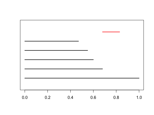
Figure 15: Barcode of the class labelled as 5B8

States in the class of Fig.15 have similar properties to those in the class of Fig.13, however in this case the $H_{1}$ homology does not persist since connections among qubits creating the hole appear at some value of $\epsilon$. An example state with such barcode could be

$$\begin{split}|5,B8\rangle=\dfrac{1}{\sqrt{10}}\left(\sqrt{5}|00000\rangle+|11000\rangle+\right.\\ \left.+|01100\rangle+|00110\rangle+|00011\rangle+|10001\rangle\right).\end{split}$$ (9)

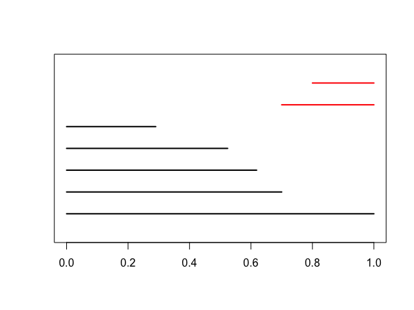
Figure 16: Barcode of the class labelled as 5B9

The class characterized by the barcode depicted in Figure 16 shows a single persistent connected component of qubits grouped by pairwise entanglement but also two holes which appear at some $\epsilon$ and persist for higher values. A representative for this class is the following

$$\begin{split}|5,B9\rangle=\sqrt{\dfrac{2}{5}}\ \left(|00000\rangle+|01010\rangle\right)+\dfrac{1}{5}\left(|00011\rangle+\right.\\ \left.+|00101\rangle+|01100\rangle+|11000\rangle+|10001\rangle\right)\end{split}$$

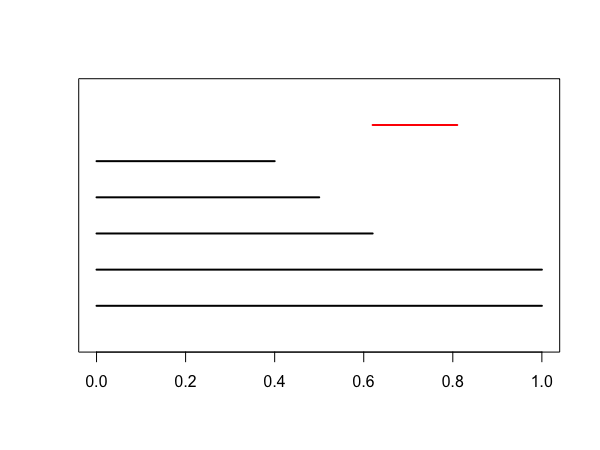
Figure 17: Barcode of the class labelled as 5B10

States belonging to the class of Figure 17 have similar properties to those in class with barcode in Figure 14, i.e. two persistent connected components, one of which is made up of a single qubit which does not share pairwise entanglement with the other four. In the other instead, the remaining four qubits get connected to form a non-persistent hole. An example state with such barcode could be

$$\begin{split}|5,B10\rangle=\dfrac{1}{\sqrt{6}}\left(|01000\rangle+|01010\rangle+\right.\\ \left.+|10000\rangle+|10001\rangle+|10110\rangle+|11010\rangle\right)\end{split}$$

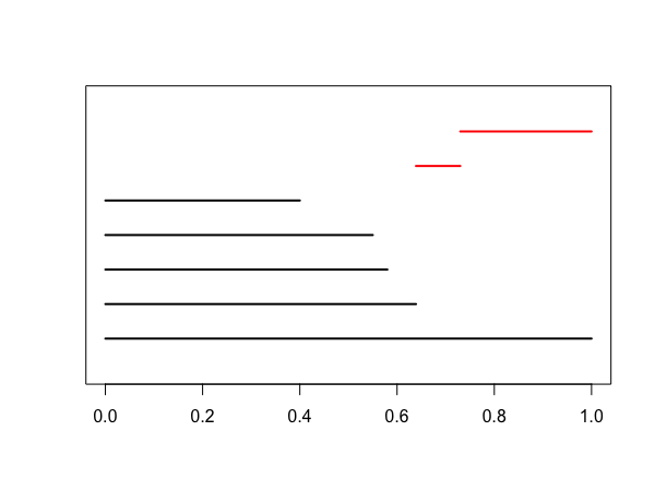
Figure 18: Barcode of the class labelled as 5B11

A single persistent connected component and two holes characterize the barcode of this class, as shown in Figure 18. Note that one of the two homology group generators $H_{1}$ appears only in a limited interval while the other one persists over $\epsilon$. An example state with such barcode:

$$\begin{split}|5,B11\rangle=\dfrac{1}{\sqrt{11}}\left(\sqrt{5}|00010\rangle+\sqrt{2}|00100\rangle+\right.\\ \left.+\sqrt{2}|10000\rangle+|10101\rangle+|11100\rangle\right)\end{split}$$

Figure 19: Barcode of the class labelled as 5B12

The least frequent class, barcode in Figure 19, is the one composed of those states where qubits get connected to form a single connected component allowing the presence of two hole that however do not persist. An example state with such barcode is the following

$$\begin{split}|5,B12\rangle=\dfrac{1}{\sqrt{2}}\ |00000\rangle+\dfrac{1}{\sqrt{10}}\left(|11000\rangle+\right.\\ \left.+|01100\rangle+|01010\rangle+|00101\rangle+|10001\rangle\right)\end{split}$$

By looking at the chart in Figure 20 it can be noticed that the most frequent barcode (5B1) belongs to states with three connected components, followed by states with barcodes showing four, two, five and one persistent components (respectively 5B2, 5B3, 5B4, 5B5). The $95\%$ of all randomly generated states fall inside one of these first five classes. After them, barcodes with higher dimensional homology features start to appear: at first those with one hole and then those with two. The only exception is given by barcode 5B10 (showing one short-lived hole but two connected components) since it is less frequent than 5B9 (one connected component and two persistent holes).

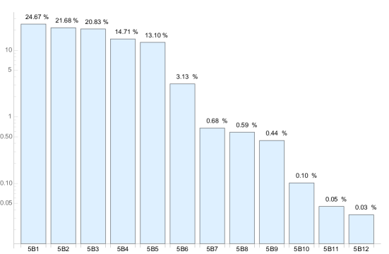
Figure 20: Barcode frequencies (in Log scale) for five qubits genuine entangled states

IV.3 Classification of six qubits states

By randomly generating six-partite genuine entangled states of six qubits, we obtained 33 different classes. Their barcodes are presented in Appendix A, while frequencies are shown in Figure 21.

With a frequency of $68\%$, the class defined by barcode 6B1 is by far the most frequent. Such a class consists of GHZ-like states that present six different connected components, i.e. the single qubits with no pairwise entanglement.

As we have seen, for the five qubit case, the first classes in frequency, from 6B1 to 6B6, are those containing states showing only connected components ($H_{0}$ homology group i.e. black bars).

Then states with one hole start to appear, and later those showing two holes, with the exception of barcodes 6B12 and 6B13.

Finally, barcodes showing multiple holes and voids, from 6B19 to 6B33 are also possible but they do not appear in the histogram since their frequency is very low ($\ll 0.004\%$).

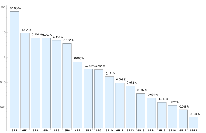
Figure 21: Barcode frequencies (in Log Scale) for six qubits genuine entangled states

V conclusion

The classification that we have carried out for four, five and six qubits entangled states shows that is possible to distinguish respectively six , twelve and thirty-three different classes by persistent homological barcodes. In general, given a $N$ qubit genuinely entangled state, it is always possible to come up with a finite classification where the total number of possible barcodes $B_{N}$ is bounded by

$$B_{N}<\left(\sum_{e=0}^{\frac{N(N-1)}{2}}G_{N}(d)\ d!\right)$$

where $G_{N}(d)$ is equal to the number of all possible graphs with $N$ vertices and $d$ edges. The factorial $d!$ is necessary to take into consideration all possible ways of building $G_{N}(d)$.

Furthermore, patterns seems to emerge in our classifications by looking at the frequencies of barcodes. First of all, those states which are characterized by the only $H_{0}$ homology group become more likely as the number of qubits $N$ increases. This is followed by the group of those states showing also $H_{1}$ which again are followed by those with a much richer topology. While this fact could be explained from a topological point of view by claiming that, with a limited number of points complex homological patterns in the barcode are harder to obtain, it is still interesting to notice that the same reasoning also hold true for quantum state barcodes.

Among those states with only the $H_{0}$ homology group, it is worth noticing that the W-like class, with only one persistent connected component, decreases its frequency with the increase of $N$. In fact, except for $N=4$ where we find this class in the first place, in the $N=5$ and $N=6$ cases, it falls to the last position. Conversely, the class of states which have $N$ persistent components, like GHZ, gradually increase their frequency, starting from the bottom at $N=4$ and becoming the most popular at $N=6$.

In general we can say that increasing the number of qubits makes the randomly generated states easily fall inside classes with more persistent connected components. This seems to indicate that, increasing the number of parties, qubits in a genuine entangled states tend to dislike pairwise entanglement and rather share it with the whole set of other qubits.

One last consideration is related to the study of quantum algorithms and their complexity classes. As quantum speed-up is essentially based on the entanglement employed in the algorithm, it would be subject of future work the study of the relation between quantum complexity classes and the persistent homology classification presented here.

Appendix A Barcodes for six-partite genuine entangled states

Here we report the 33 different barcodes obtained from randomly generated six-partite genuine entangled states. As usual, barcodes are presented starting from the most frequent to the least frequent one.

6B1

6B2

6B3

6B4

6B5

6B6

6B7

6B8

6B9

6B10

6B11

6B12

6B13

6B14

6B15

6B16

6B17

6B18

6B19

6B20

6B21

6B22

6B23

6B24

6B25

6B26

6B27

6B28

6B29

6B30

6B31

6B32

6B33

References

- (1) M. Walter, D. Gross, and J. Eisert, arXiv:1612.02437 (2017).
- (2) G. Vidal, Journal of Modern Optics, 47, 2-3 (2000).
- (3) R. Horodecki, et al. Reviews of Modern Physics 81, 865 (2009).
- (4) W. Dur, G. Vidal, and J. I. Cirac, Physical Review A 62, 062314 (2000).
-
(5)
F. Verstraete, J. Dehaene, B. De Moor, and H. Verschelde,
Physical Review A 65, 052112 (2002);
Y. Cao, and A. M. Wang, European Physical Journal D 44, 159 (2007);
M. Gharahi and S. J. Akhtarshenas, European Physical Journal D 70, 54 (2016). - (6) G. M. Quinta, and A. Rui, Physical Review A 97, 042307 (2018).
- (7) A. Di Pierro, S. Mancini, L. Memarzadeh, and R. Mengoni, Europhysics Letters 123, 30006 (2018).
- (8) H. Edelsbrunner, D. Letscher and A. Zomorodian, Discrete Computational Geometry, 28, 511 (2002).
- (9) G. Carlsson, and A. Zomorodian, Discrete Computational Geometry 33, 249 (2005).
- (10) A. Hatcher, Algebraic Topology, Cambridge University Press (2002).
- (11) H. Edelsbrunner, A Short Course in Computational Geometry and Topology, Springer Publishing Company (2014).
- (12) R. Ghrist, Bulletin of the American Mathematical Society, 45, 1 (2008).
- (13) K. Zyczkowski, and H. J. Sommers, Journal of Physics A: Mathematical and General 34, 35 (2001).
- (14) L. Memarzadeh, and S. Mancini, Physical Review A 94, 022341 (2016).
- (15) W. K. Wootters, Quantum Information & Computation 1, 1 (2001).
- (16) S. Hill, and W. K. Wootters, Physical Review Letters 78, 26 (1997).