Non-Abelian braiding of Majorana-like edge states and
topological quantum computations in electric circuits

Abstract

Majorana fermions subject to the non-Abelian braid group are believed to be the basic ingredients of future topological quantum computations. In this work, we propose to simulate Majorana fermions of the Kitaev model in electric circuits based on the observation that the circuit Laplacian can be made identical to the Hamiltonian. A set of AC voltages along the chain plays a role of the wave function. We generate an arbitrary number of topological segments in a Kitaev chain. A pair of topological edge states emerge at the edges of a topological segment. Its wave function is observable by the position and the phase of a peak in impedance measurement. It is possible to braid any pair of neighboring edge states with the aid of T-junction geometry. By calculating the Berry phase acquired by their eigenfunctions, the braiding is shown to generate one-qubit and two-qubit unitary operations. We explicitly construct Clifford quantum gates based on them. We also present an operator formalism by regarding a topological edge state as a topological soliton intertwining the trivial segment and the topological segment. Our analysis shows that the electric-circuit approach can simulate the Majorana-fermion approach to topological quantum computations.

I Introduction

The braiding relation plays a key role in future topological quantum computationsMoore ; Das ; Kitaev ; TQC ; SternA ; Stern ; NPJ ; Bonder ; Cheng ; Pahomi . Majorana-fermion edge states emerging in topological superconductors are the best candidateAliceaBraid ; Qi ; Alicea ; Lei ; Been ; Stan ; Elli ; Sato ; Les ; AA ; DJ ; Ivanov ; Halperin ; Sni . Examples are the $p_{x}+ip_{y}$ topological superconductorsIvanov and the Kitaev $p$-wave topological superconductorsAliceaBraid ; DJ . However, an experimental realization of braiding of Majorana fermions still remains challenging.

The study on topological phases started in condensed-matter physicsHasan ; Qi , but now expanded to other systems including acousticTopoAco ; Berto ; Sss ; He , photoicKhaniPhoto ; Hafe2 ; Hafezi ; WuHu ; TopoPhoto ; Ozawa , mechanicalNash ; Huber and electric-circuitTECNature ; ComPhys systems. In particular, almost all topological phases are known to be materialized in electric circuits because the circuit Laplacian has the same expression as the Hamiltonian when the circuit is appropriately designedTECNature ; ComPhys , where the admittance corresponds to the energy. Very recently, we have generated Majorana-like corner states akin to those in topological superconductors and shown that the braiding of these Majorana-like corner states is possible in electric circuitsEzawaMajo . Indeed, we have derived the relation $\sigma^{2}=-1$, where $\sigma$ denotes a single exchange of two topological corner states. It indicates that a topological corner state is an Ising anyon. Note that the relation $\sigma^{2}=1$ holds both for bosons and fermions. However, the single exchange $\sigma$ is impossible in this model. This is because the braiding is controlled by an applied field and the direction of the field becomes opposite after a single braid. Another problem is that it is not clear how to braid more than two topological corner states.

In this paper, employing the electric-circuit realization of the Kitaev modelEzawaMajo , we generate $N$ topological segments together with $N$ pairs of topological edge states in a Kitaev chain made of electric circuit. We describe them by $N$ pairs of wave functions $(\vec{\psi}_{A}^{j},\vec{\psi}_{B}^{j})$, $j=1,2,\cdots,N$, as in Fig.1. All pairs $(\vec{\psi}_{A}^{j},\vec{\psi}_{B}^{j})$ are orthogonal one to another, since all topological segments are independent from one to another, thus yielding $2^{N}$-fold degeneracy of the topological edge states.

The position and the phase of one edge state are observable by those of a peak in impedance measurement. It is possible to carry out the braiding of edge states with the use of T-junctionsAliceaBraid ; AA . Furthermore, we demonstrate that the braiding of two edge states across a topological (trivial) segment generates one-qubit (two-qubit) unitary operation.

It is interesting to develop our scheme to pursue to what extent the electric-circuit formalism can simulate the standard Majorana-operator formalism. For this purpose, we remark that it is possible to regard a topological edge state as a topological soliton because it intertwines the topological and the trivial segments. Let us call it an edge soliton when we focus on the aspect of soliton. We then define an operator that creates an edge soliton. Remarkably, it behaves as a Majorana-fermion operator in the electric-circuit formalism.

The paper is composed as follows. In Sec. II, we focus on a single topological segment together with a pair of edge solitons. A pair of wave functions $\vec{\psi}_{A}$ and $\vec{\psi}_{B}$ are analytically constructed to describe it. One-qubit states are described by superpositions of $\vec{\psi}_{A}$ and $\vec{\psi}_{B}$.

In Sec. III, we review the electric-circuit realization of the Kitaev model. A circuit consists of two main channels, i.e., the capacitor channel and the inductor channel, corresponding to the electron band and the hole band in the Kitaev model. It is shown that an edge soliton is observable by an impedance peak both in these two channels, whose phase agrees precisely with that of the wave function $\vec{\psi}_{A}$ or $\vec{\psi}_{B}$. We also discuss how to register and observe the qubit information in the electric circuit.

In Sec. IV, we investigate the braiding of edge states. First, we analyze how the eigenfunction evolves when some system parameters are locally controlled. In particular, the Berry phase develops when the "superconducting-phase" parameter is externally controlled. Then, using these results, we investigate the braiding of two edges across a topological segment and also across a trivial segment. Their effect is represented as one-qubit and two-qubit unitary operators, respectively. We explicitly construct Clifford quantum gates based on them.

In Sec. V and VI, we introduce a creation operator $\gamma_{j}$ of an edge soliton described by the wave function $\vec{\psi}_{j}$. It is argued that $\gamma_{j}$ is a Majorana-fermion operator by investigating the exchange statistics of two edge solitons. All results are in consistent with those derived by the analysis of the Berry phase.

In Sec. VII, we present explicit formulas for the electric-circuit realization of the Kitaev model by deriving the circuit Laplacian to be identified with the Kitaev Hamiltonian. We also present an electric circuit for a T-junction. Sec. VIII is devoted to discussions.

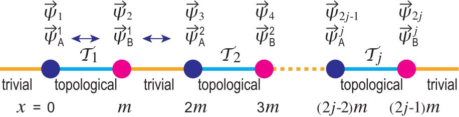
Figure 1: We create a number of topological segments on a single Kitaev chain by controlling the chemical potential locally. A pair of topological zero-energy states emerge at the edges of the $j$-th topological segment $\mathcal{T}_{j}$ (cyan). Their wave functions are denoted by $\vec{\psi}_{A}^{j}$ and $\vec{\psi}_{B}^{j}$. We may relabel them as $(\vec{\psi}_{A}^{1},\vec{\psi}_{B}^{1},\vec{\psi}_{A}^{2},\vec{\psi}_{B}^{2},\cdots)\rightarrow(\vec{\psi}_{1},\vec{\psi}_{2},\vec{\psi}_{3},\vec{\psi}_{4},\cdots)$. We investigate two basic braids: (i) We braid two edge states $\vec{\psi}_{A}^{1}$ and $\vec{\psi}_{B}^{1}$ across a topological segment, leading to a unitary operation in one qubit. (ii) We braid two edge states $\vec{\psi}_{B}^{1}$ and $\vec{\psi}_{A}^{2}$ across a trivial segment, leading to a unitary operation in two qubits. For definiteness, it is assumed that each topological segment contains $m+1$ sites while each trivial segment contains $m-1$ sites. The site index is expressed as $x=0,1,2,\cdots$. Edge states emerge at $x=0,m,2m,\cdots$.

II Kitaev model

The Bogoliubov-de Gennes Hamiltonian is written as

$$\hat{H}(\boldsymbol{k})=\Psi^{{\dagger}}(\boldsymbol{k})H(\boldsymbol{k})\Psi(\boldsymbol{k}),$$ (1)

with the Nambu operator

$$\Psi(\boldsymbol{k})=\left\{c(\boldsymbol{k}),c^{\dagger}(\boldsymbol{k})\right\}.$$ (2)

It is customary to refer to $H(\boldsymbol{k})$ also as the Hamiltonian. The Hamiltonian $H(k)$ may be regarded as a classical Hamiltonian, whereas $\hat{H}(k)$ is a second-quantized Hamiltonian. Topological properties of the system are determined by the property of the classical Hamiltonian $H(k)$.

The Kitaev $p$-wave topological superconductor model is the fundamental one-dimensional model hosting Majorana edge statesRead ; KitaevP ; Kitaev ; Alicea . It is a two-band model whose Hamiltonian is

$$H_{\text{K}}(k)=\frac{1}{2}\left(\begin{array}[]{cc}\varepsilon_{k}&i\Delta e^{-i\phi}\sin k\\ -i\Delta e^{i\phi}\sin k&-\varepsilon_{k}\end{array}\right),$$ (3)

with

$$\varepsilon_{k}=-t\cos k-\mu,$$ (4)

where $t$, $\mu$, $\phi$ and $\Delta$ represent the hopping amplitude, the chemical potential, the superconducting phase and gap parameters, respectively. It is well known that the system is topological for $\left|\mu\right|<\left|2t\right|$ and trivial for $\left|\mu\right|>\left|2t\right|$ irrespective of $\Delta$ provided $\Delta\neq 0$. A pair of topological zero-energy states emerges at the edges of a topological phase according to the bulk-edge correspondence. They are protected by particle-hole symmetry (PHS).

We consider a chain realizing the Kitaev model. A chain need not be straight; it can bend or even branch off. We control the system parameters locally so as to generate several topological segments with $\left|\mu\right|<\left|2t\right|$ sandwiched by trivial segments with $\left|\mu\right|>\left|2t\right|$ as in Fig.1.

It is convenient to choose the parameters such that

$$\Delta=t,\text{\qquad}\mu=0$$ (5)

to generate a topological segment, and

$$\Delta=t,\text{\qquad}\mu=4t$$ (6)

to generate a trivial segment. Then, we obtain analytical solutions describing the zero-energy edge states as in Eqs.(13).

The Kitaev model (3) is reduced to

$$H_{\text{K}}^{y}(k)=\frac{1}{2}\varepsilon_{k}\sigma_{z}-\frac{1}{2}\Delta\sigma_{y}\sin k$$ (7)

for $\phi=0$, and

$$H_{\text{K}}^{x}(k)=\frac{1}{2}\varepsilon_{k}\sigma_{z}+\frac{1}{2}\Delta\sigma_{x}\sin k.$$ (8)

for $\phi=\pi/2$. In the present work, we use the $H_{\text{K}}^{y}$ model (7), where $\phi=0$. However, this phase degree of freedom plays a key role when we braid two edge states. The system parameters $t$, $\mu$, $\phi$ and $\Delta$ are locally controllable parameters in the corresponding circuit Laplacian.

II.1 Zero-energy solutions

To obtain analytic solutions of the zero-energy states, we make a unitary transformation of the Kitaev model (3) as $H_{\text{K}}^{\prime}\left(k\right)=U_{\text{K}}H_{\text{K}}\left(k\right)U_{\text{K}}^{-1}$ with

$$U_{\text{K}}=\frac{1}{\sqrt{2}}\left(\begin{array}[]{cc}-ie^{i\phi/2}&ie^{-i\phi/2}\\ e^{i\phi/2}&e^{-i\phi/2}\end{array}\right),$$ (9)

and obtain

$$H_{\text{K}}^{\prime}\left(k\right)=\frac{1}{2}\left(\begin{array}[]{cc}0&-i\varepsilon_{k}+\Delta\sin k\\ i\varepsilon_{k}+\Delta\sin k&0\end{array}\right).$$ (10)

With the choice (5) of the parameters, it is simplified as

$$H_{\text{K}}^{\prime}\left(k\right)=\frac{1}{2}\left(\begin{array}[]{cc}0&ite^{-ik}\\ -ite^{ik}&0\end{array}\right).$$ (11)

When one topological segment contains $m+1$ sites, the zero-energy solutions of this model are explicitly given in the coordinate space by

$$\vec{\psi}_{A}^{\prime}=\left(1,0,\cdots,0\right),\qquad\vec{\psi}_{B}^{\prime}=\left(0,\cdots,0,1\right),$$ (12)

which are $2(m+1)$ component vectors.

By making the inverse unitary transformation, we obtain the zero-energy solutions in the original Kitaev Hamiltonian (3) as

$$\vec{\psi}_{A} =U_{\text{K}}^{-1}\vec{\psi}_{A}^{\prime}$$

$$=\frac{1}{\sqrt{2}}(ie^{-i\phi/2},0,\cdots,0;-ie^{i\phi/2},0,\cdots,0),$$

$$\vec{\psi}_{B} =U_{\text{K}}^{-1}\vec{\psi}_{B}^{\prime}$$

$$=\frac{1}{\sqrt{2}}(0,\cdots,0,e^{-i\phi/2};0,\cdots,0,e^{i\phi/2}),$$ (13)

where $\phi$ is the superconducting phase in the Hamiltonian (3). We refer to the first (last) $(m+1)$-components as the electron (hole) sector in accord with the Nambu operator (2). It is seen that $\vec{\psi}_{A}$ and $\vec{\psi}_{B}$ are perfectly localized at the left edge and the right edge, respectively. They agree with the wave functions of the Majorana edge states in the Kitaev $p$-wave topological superconductor model.

II.2 One-qubit state

We analyze a Kitaev chain containing one topological segment, where there are two topological edge states $\vec{\psi}_{A}$ and $\vec{\psi}_{B}$. Any linear combination of $\vec{\psi}_{A}$ and $\vec{\psi}_{B}$ is degenerate at zero energy. We construct a set of orthogonal states $\vec{\psi}_{|0\rangle}$ and $\vec{\psi}_{|1\rangle}$ as

$$\left(\begin{array}[]{c}\vec{\psi}_{|0\rangle}\\ \vec{\psi}_{|1\rangle}\end{array}\right)=U_{\text{basis}}\left(\begin{array}[]{c}\vec{\psi}_{A}\\ \vec{\psi}_{B}\end{array}\right),$$ (14)

with

$$U_{\text{basis}}=\frac{1}{\sqrt{2}}\left(\begin{array}[]{cc}1&i\\ 1&-i\end{array}\right),$$ (15)

which read

$$\vec{\psi}_{|n\rangle} =\frac{i}{2}\{e^{-i\phi/2},\cdots,0,\left(-1\right)^{n}e^{-i\phi/2};$$

$$\qquad\qquad-e^{i\phi/2},\cdots,0,\left(-1\right)^{n}e^{i\phi/2}\},$$ (16)

where $n=0,1$. As far as the electron sector concerns, the wave function $\vec{\psi}_{|0\rangle}$ is symmetric with respect to the change of the components at $x=0$ and $x=m$, while $\vec{\psi}_{|1\rangle}$ is antisymmetric. We later show that $\vec{\psi}_{|0\rangle}$ and $\vec{\psi}_{|1\rangle}$ are the wave functions describing one-qubit states $|0\rangle$ and $|1\rangle$, respectively: See Eq.(120).

In application of the Kitaev model for quantum computation we start from and end at the system with the "superconducting phase" $\phi=0$, where

$$\vec{\psi}_{|n\rangle}=\frac{i}{2}(1,0,\cdots,0,\left(-1\right)^{n};-1,0,\cdots,0,\left(-1\right)^{n}).$$ (17)

We make the use of the phase degrees of freedom only when we perform braiding of edge states.

II.3 Multi-qubit state

We proceed to consider a Kitaev chain containing $N$ topological segments, where the $j$-th topological segment produces two topological edge states described by the wave functions $\vec{\psi}_{A}^{j}$ and $\vec{\psi}_{B}^{j}$ as in Fig.1. We may construct a set of wave functions $\vec{\psi}_{|0\rangle}^{j}$ and $\vec{\psi}_{|1\rangle}^{j}$ as in Eq.(14), describing one-qubit states $|0\rangle_{j}$ and $|1\rangle_{j}$ for the $j$-th topological segment. They are orthogonal and degenerate at zero energy, forming a two-dimensional Hilbert space $\mathcal{T}_{j}$. When there are $N$ topological segments, the total Hilbert space is the direct product of $N$ Hilbert spaces, that is $\otimes_{j}\mathcal{T}_{j}$. The many-body ground states are given by the direct product,

$$\left|n_{1}n_{2}\cdots n_{N}\right\rangle=\left|n_{1}\right\rangle_{1}\otimes\left|n_{2}\right\rangle_{2}\otimes\cdots\otimes\left|n_{N}\right\rangle_{N}$$ (18)

with $n_{j}=0,1$, where the index $j$ denotes the $j$-th topological segment. The ground-state degeneracy is $2^{N}$ as in the case of topological superconductors, although we have derived it solely based on the classical Hamiltonian.

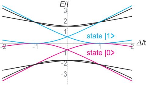
Figure 2: Energy $E/t$ as a function of $\Delta/t$ for a finite chain with length 4. The two zero-energy states split and acquire nonzero energy for $t\neq\Delta$.

II.4 Initialization

It is standard to start with the pure state $\left|00\cdots 0\right\rangle$ to carry out quantum computation. Such a pure state can be prepared as follows. We first tune the "superconducting" gap $|\Delta|$ slightly larger than the hopping amplitude $|t|$, $|\Delta/t|>1$, in a topological segment. Although the two-fold degeneracy of the state $\left|0\right\rangle$ and the state $\left|1\right\rangle$ is intact in an infinitely long system due to the PHS, it is broken in a finite system because there is a mixing between the two edge states. The energy of the state $\left|0\right\rangle$ becomes lower than that of the state $\left|1\right\rangle$, as numerically shown in Fig.2 for a finite chain with length 4. Thus, we can choose the state $\left|0\right\rangle$. By doing this setup for all topological phases, we can construct the pure state $\left|00\cdots 0\right\rangle$.

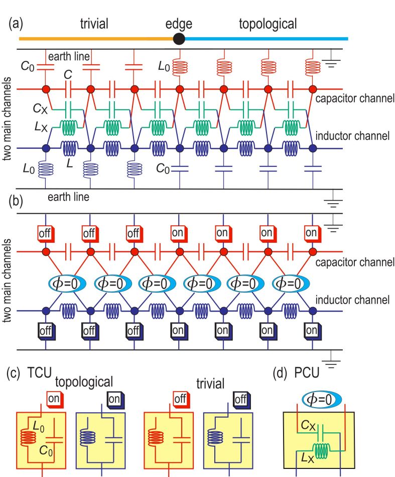
Figure 3: (a) A topological edge state emerges at the boundary between a trivial and a topological segment. This Kitaev chain is simulated by a set of two channels containing capacitors C (red) and inductors L (blue), corresponding to the electron band and the hole band, respectively. Each site is connected to the ground via a capacitor ($C_{0}$) or an inductor ($L_{0}$) to realize trivial and topological segments as shown in this figure. In the model with $\phi=0$, the two main channels are crosslinked by a circuit composed of capacitors ($C_{X}$) and inductors ($L_{X}$). (b) The same Kitaev chain is illustrated in terms of the TCU (topology-control unit) and the PCU (phase-control unit) with $\phi=0$. (c) Illustration of TCU. (d) Illustration of PCU at $\phi=0$.

III Electric-circuit realization

Electric circuits can simulate various topological systemsTECNature ; ComPhys ; Hel ; Lu ; Research ; Zhao ; EzawaTEC ; Garcia ; Hofmann ; EzawaLCR ; Haenel ; EzawaSkin ; XiaoXiao . We review how to realize the Kitaev model by an electric circuitEzawaMajo . We use two main channels (red and blue) to represent a two-band model as in Fig.3(a): One channel (i.e., capacitor channel) consists of capacitors $C$ in series, implementing the electron band, while the other channel (i.e., inductor channel) consists of inductors $L$ in series, implementing the hole band. The hopping parameters are represented by capacitors $C$ and inductors $L$, whose contribution to the circuit Laplacian is $i\omega C$ and $1/i\omega L$: See Eq.(20). It is understood that the hopping parameters are opposite between the electron band and the hole band. We then introduce a pairing interaction between them, by crosslinking the two main channels with the use of capacitors $C_{X}$ and inductors $L_{X}$, as shown in green in Fig.3(a). Each site in the main channel is connected to the ground via an inductor $L_{0}$ or a capacitor $C_{0}$ as shown in Fig.3(a). The use of $C_{0}$ in the capacitor channel and $L_{0}$ in the inductor channel makes the segment trivial, while the use of $L_{0}$ in the capacitor channel and $C_{0}$ in the inductor channel makes the segment topological.

It is convenient to simplify Fig.3(a) down to Fig.3(b), where we have introduced subcircuits called the topology-control unit (TCU) and the phase-control unit (PCU) explained in Figs.3(c) and (d). When all TCUs are set on (off) in a segment, the segment is in the topological (trivial) phase. A topological edge state emerges at an edge site of a topological segment. By switching on a TCU attached to the adjacent site, a topological edge state is shifted to the adjacent site. Namely, we can move a topological edge state freely along a Kitaev chain. In a braiding process of two edge states, as we explain in Sec.VII.3, it is necessary to control the "superconducting phase" $\phi$ present in the Kitaev model (3), which is controlled with the use of PCUs.

III.1 Circuit Laplacian

Electric circuits are characterized by the Kirchhoff current lawTECNature ; ComPhys ; Hel ,

$$\frac{d}{dt}I_{a} =\sum_{b}C_{ab}\frac{d^{2}}{dt^{2}}\left(V_{a}-V_{b}\right)+\frac{1}{L_{0}}V_{a}$$

$$+\sum_{b}\frac{1}{L_{ab}}\left(V_{a}-V_{b}\right)+C_{0}\frac{d^{2}}{dt^{2}}V_{a},$$ (19)

where $I_{a}$ is the current between site $a$ and the ground, $V_{a}$ is the voltage at site $a$, $C_{ab}$ is the capacitance and $L_{ab}$ is the inductance between sites $a$ and $b$, and the sum is taken over all adjacent sites $b$, while $L_{0}$ is the inductance and $C_{0}$ is the capacitance between site $a$ and the ground.

By making the Fourier transformation, $I_{a}\left(t\right)=I_{a}\left(\omega\right)e^{i\omega t}$ and $V_{a}\left(t\right)=V_{a}\left(\omega\right)e^{i\omega t}$, the Kirchhoff current law leads to the formulaComPhys ; TECNature ,

$$I_{a}\left(\omega\right) =\sum_{b}i\omega C_{ab}\left(V_{a}-V_{b}\right)+\frac{1}{i\omega L_{0}}V_{a}$$

$$+\sum_{b}\frac{1}{i\omega L_{ab}}\left(V_{a}-V_{b}\right)+i\omega C_{0}V_{a},$$ (20)

which is summarized as

$$I_{a}\left(\omega\right)=\sum_{b}J_{ab}\left(\omega\right)V_{b}\left(\omega\right),$$ (21)

where the sum is taken over all adjacent sites $b$. Here, $J_{ab}\left(\omega\right)$ is called the circuit Laplacian.

We present a detailed analysis of the circuit Laplacian $J_{ab}\left(\omega\right)$ in Sec.VII as in Eq.(131). We equate the circuit Laplacian with the classical Kitaev Hamiltonian (3),

$$J_{ab}\left(\omega\right)=i\omega H_{ab}\left(\omega\right).$$ (22)

The relation between the parameters in the Kitaev model and in the electric circuit are determined by this formula.

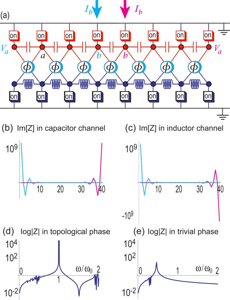
Figure 4: Kitaev chain in the topological phase. When the current is injected at the magenta (cyan) site $b$ in (a), the impedance $Z_{ab}$ is given by a magenta (cyan) curve as a function of the site $a$ in (b) and (c). An impedance peak appears in Im[$Z_{ab}$] as indicated in (b) and (c), when we take the site $a$ in the capacitor channel and the inductor channel, respectively. The frequency is taken at the critical one $\omega_{0}$. (d) Impedance is given as a function of $\omega/\omega_{0}$. A huge peak appears at the critical one in the topological phase ($\mu=0$). (e) There is no peak at $\omega=\omega_{0}$. in the trivial phase ($\mu=4t$). We have considered a Kitaev chain containing $40$ sites, and we have set $\Delta=0.9t$.

In general, the voltage is uniquely determined in terms of the current by the Kirchhoff law (21). However, this is not the case for the zero-energy sector, for which we obtain

$$\sum_{b}H_{ab}\left(\omega\right)\Psi_{b}\left(\omega\right)=0,$$ (23)

where we have identified the voltage function,

$$\Psi(\omega) =\frac{1}{\sqrt{\sum_{a}|V_{a}|^{2}}}(\cdots,V_{0}^{e},V_{1}^{e},\cdots,V_{m}^{e},\cdots;$$

$$\quad\quad\quad\quad\cdots,V_{0}^{h},V_{1}^{h},\cdots,V_{m}^{h},\cdots)$$ (24)

as the wave function. Here, $V_{0}^{e}$ and $V_{m}^{e}$ ($V_{0}^{h}$ and $V_{m}^{h}$) are the voltages at the edges in the electron (hole) sector of the topological segment $\mathcal{T}_{1}$ in the Kitaev chain in Fig.1.

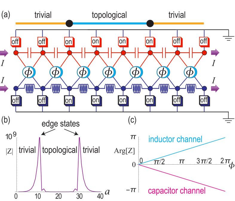
Figure 5: (a) Electric circuit for a Kitaev chain with a topological segment and two adjacent trivial segments. (b) Absolute value of the impedance resonance at the critical frequency $\omega_{0}$, showing the emergence of a pair of topological edge states in a Kitaev chain containing $40$ sites. They are located at the site $a=11$ and $a=30$. We take $\Delta/t=0.9$ for illustration. The peaks become strictly localized for $\Delta/t=1$. (c) $\phi$ dependence of Arg$\left[Z\right]$ for the edge state in the capacitor channel (magenta) and the inductor channel (cyan).

III.2 Impedance peak

The emergence of a pair of topological edge states is observed electrically by feeding an external current to the chain. Since they are the zero-energy eigenstate of the Kitaev Hamiltonian and since the energy corresponds to the admittance, their emergence is observable by peaks in the impedance. The impedance between the $a$ and $b$ sites is given byHel $Z_{ab}^{\left(1\right)}\equiv V_{a}/I_{b}=G_{ab}$, where $G$ is the Green function defined by the inverse of the Laplacian $J$, $G\equiv J^{-1}$.

First, we show the impedance $Z_{ab}^{\left(1\right)}$ for a finite Kitaev chain in a topological phase as a function of the site $a$, when a current is injected from the site $b$ at the center of the chain, as shown in Fig.4(a). When $b$ is on the even (odd) site, the impedance takes the maximum at the left (right) side of the chain as in Fig.4(b) and (c). We show the impedance at the edge as a function of $\omega/\omega_{0}$ for the topological and trivial phases in Fig.4(d) and (e). There is a strong resonance at the critical frequency at $\omega=\omega_{0}$ only in the topological phase, showing the emergence of a zero-admittance state in the topological phase.

Next, we consider a Kitaev chain containing one topological segment sandwiched by two trivial segments. As in Fig.5(a), we inject the current $Ie^{i\omega t}$ from the left-hand side of the two main channels and subtract it from the right-hand side. In Fig.5(b), we show the impedance of a finite Kitaev chain as a function of the site $a$ in the capacitor (inductor) channel, which is calculated by

$$Z_{a}=V_{a}/I=G_{a\text{L}}-G_{a\text{R}},$$ (25)

where L denotes the left-most site in the capacitor (inductor) channel and R denotes the right-most site in the capacitor (inductor) channel. There are peaks at the edges of the topological segment. The penetration depth is longer in the trivial phases than that in the topological phase. In Fig.5(c), we show the angle of the impedance peak at the critical frequency, which is well fitted by the lines

$$\text{arg}\left[Z_{a}\left(\phi\right)\right]=\log\left(Z_{a}/\left|Z_{a}\right|\right)=\pm\frac{1}{2}\phi$$ (26)

for the capacitor channel ($-$) and the inductor channel ($+$) at an edge site. Thus, the "superconducting" phase $\phi$ is observable in the capacitor channel (magenta) and the inductor channel (cyan), as indicated by the zero-energy solutions (13) of the Kitaev model.

III.3 LC resonator as information storage

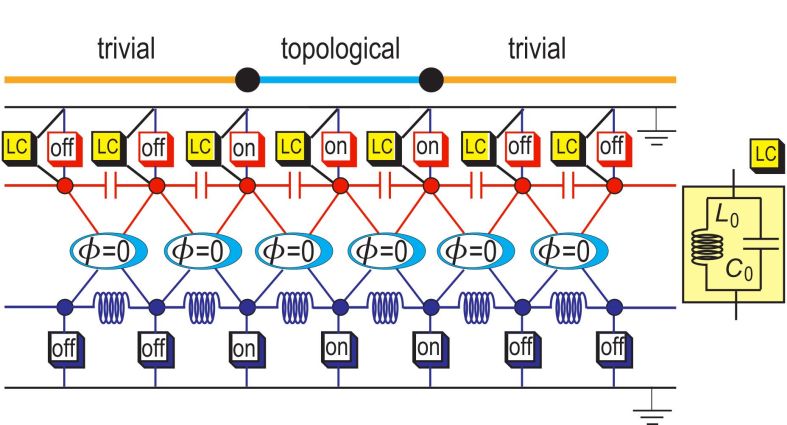
Figure 6: We attach an LC resonator to each site to register the phase of voltage in the capacitor channel.

The emergence of an edge state is observed by an impedance peak when a current $Ie^{i\omega t}$ is injected. However, in performing a braiding operation, we should not inject any external current since it may affect the phase of the voltage externally. We wonder how to register and observe the qubit information in electric circuits.

It is possible to store the qubit information in LC resonators, which are to be inserted to the Kitaev chain, as illustrated in Fig.6. It is enough to introduce LC resonators only to the capacitor channel, because the voltages in the two channels are related by complex conjugation.

An LC resonator is described by the Kirchhoff law,

$$I_{C}+I_{V}=0,\qquad I_{C}=C_{0}\frac{dV_{C}}{dt},\qquad V_{L}=L_{0}\frac{dI_{L}}{dt},$$ (27)

which amount to

$$\frac{d^{2}I}{dt^{t}}+\omega_{0}^{2}I=0$$ (28)

at the critical frequency $\omega_{0}=1/\sqrt{L_{0}C_{0}}$. The solution is given by

$$I=I_{0}\sin\left(\omega_{0}t+\theta_{0}\right),\qquad V=V_{0}\cos\left(\omega_{0}t+\theta_{0}\right),$$ (29)

where $\theta_{0}$ is an initial phase at $t=0$. In the Fourier form, the contribution of the LC resonator to the circuit Laplacian (131) is given by

$$J=i\omega_{0}C_{0}+\frac{1}{i\omega_{0}L_{0}}=0$$ (30)

at the critical frequency. Hence, the edge states are not affected by the insertion of the LC resonator.

Furthermore, because the impedance diverges at the edge states, there is a perfect reflection at the edge states. Thus, even when we activate an LC resonator connected with an edge state, the current circularly loops only within the LC resonator. Nevertheless, the voltage of an edge state is naturally the same as that of an LC resonator.

We consider a pair of LC resonators attached to the right and left edges of one topological segment. Let us choose the phase of the voltage such as $(\theta_{A},\theta_{B})=(0,0)$ or $(0,\pi)$ in the capacitor channel. Substituting these into Eq.(29) we obtain

$$V(\theta_{A},\theta_{B}) =\frac{iV_{0}\cos\left(\omega_{0}t\right)}{2}$$

$$\times(1,0,\cdots,0,\left(-1\right)^{n};-1,0,\cdots,0,\left(-1\right)^{n}),$$ (31)

where $n=0$ for $(\theta_{A},\theta_{B})=(0,0)$, or $n=1$ for $(\theta_{A},\theta_{B})=(0,\pi)$. After normalization, we obtain

$$\vec{\psi}_{|n\rangle}=\frac{i}{2}(1,0,\cdots,0,\left(-1\right)^{n};-1,0,\cdots,0,\left(-1\right)^{n}),$$ (32)

which agrees with the wave function (17) for the one-qubit states $|0\rangle$ and $|1\rangle$. As far as the electron sector concerns, they are in-phase and opposite-phase states. Hence, one-qubit information can be registered in a pair of resonators as the in-phase state $\left|0\right\rangle$ or the opposite-phase state $\left|1\right\rangle$. Generalization to the system having $N$ topological segments is straightforward.

Figure 7: Illustrations of a braiding process of the two edges across a topological segment (cyan) with the use of a T-junction. The two edges in the initial configuration (a) are braided into those in the final configuration (i). Arrows $\rightarrow,\uparrow$ and $\leftarrow,\downarrow$ on the legs represent the phase $\phi=0$ and $\phi=\pi$, respectively. The phase is rotated from $\phi=0$ to $\phi=\pi$ between (d) to (e), and from $\phi=\pi$ to $\phi=0$ between (h) to (i). Long arrows beside legs indicate the direction toward which an edge is moved.

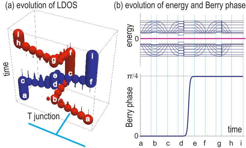
Figure 8: (a) Evolution of the local density of states (LDOS) describing the two edges of a topological segment. The evolution is smooth. (b) Evolution of the energy and the Berry phase as a function of time. The zero-energy edge states (red line) are well separated from the bulk states (blue curves) during the braiding process. Both edges acquire the Berry phase $\pi/4$ during the process (d) to (e) in Fig.7. Each leg has five sites. Alphabets a,b, $\cdots$, i denotes the steps (a), (b), $\cdots$, (i) of the braiding process in Fig.7.

IV Braiding process

IV.1 Berry phase

We investigate how a set of eigenfunctions describing a pair of edge states evolves when a system parameter is locally modified from an initial value $\Omega_{0}$ to another value $\Omega$.

Let $\vec{\psi}_{\beta}(\Omega)_{\text{initial}}$ be the zero-energy eigenfunction of the Hamiltonian $H(\Omega)$,

$$H(\Omega)\vec{\psi}_{\beta}(\Omega)_{\text{initial}}=0.$$ (33)

As $\Omega$ changes, it evolves asTQC ; Kitaev ; NPJ ; Bonder ; Cheng ; Pahomi ; EzawaMajo

$$\vec{\psi}_{\alpha}(\Omega)=U^{\alpha\beta}(\Omega,\Omega_{0})\vec{\psi}_{\beta}(\Omega)_{\text{initial}},$$ (34)

where

$$U(\Omega,\Omega_{0})=e^{i\Gamma(\Omega,\Omega_{0})},$$ (35)

with $\Gamma\left(\Omega,\Omega_{0}\right)$ the Berry phaseWilczek defined by

$$\Gamma_{\alpha\beta}\left(\Omega,\Omega_{0}\right)=-i\int_{\Omega_{0}}^{\Omega}\vec{\psi}_{\alpha}^{{\dagger}}d\vec{\psi}_{\beta}.$$ (36)

Here, $\vec{\psi}_{\alpha}$ is the electron-sector part of the eigenfunction in Eq.(13). The Berry phase accumulation is opposite between the electron and hole sectors, as follows from the PHS.

We consider two basic examples. First, we control the phase $\phi$ locally. Let us choose $\phi=0$ for the initial state. When it increases from $\phi=0$ to $\phi=\Phi$, the Berry phase is

$$\Gamma_{\alpha\beta}\left(\Phi\right)=-i\int_{0}^{\Phi}\vec{\psi}_{\alpha}^{{\dagger}}(\phi)\partial_{\phi}\vec{\psi}_{\beta}(\phi)d\phi=\delta_{\alpha\beta}\frac{\Phi}{4},$$ (37)

where we have used $\vec{\psi}_{\alpha}^{{\dagger}}(\phi)\partial_{\phi}\vec{\psi}_{\beta}(\phi)=(i/4)\delta_{\alpha\beta}$.

Second, we control the length of a topological segment by tuning locally the chemical potential $\mu$. We obtain $\Gamma_{\alpha\beta}=0$ when we shift the position of an edge without changing the phase $\phi$. For example, we consider the following states in the range $0\leq x\leq\pi/2$,

$$\vec{\psi}_{A}\left(x\right)= \frac{1}{\sqrt{2}}\{e^{-i\phi/2}\cos x,e^{-i\phi/2}\sin x,\cdots,0;$$

$$\qquad\qquad e^{i\phi/2}\cos x,e^{i\phi/2}\sin x,\cdots,0\},$$

$$\vec{\psi}_{B}\left(x\right)= \frac{1}{\sqrt{2}}\{0,\cdots,-ie^{-i\phi/2}\sin x,-ie^{-i\phi/2}\cos x;$$

$$\qquad\qquad 0,\cdots,ie^{i\phi/2}\sin x,ie^{i\phi/2}\cos x\}.$$ (38)

They describe the edge states (13) when $x=0$. As $x$ increases from $x=0$ to $x=\pi/2$, the edge moves just by one site. Then we find $\vec{\psi}_{\alpha}^{{\dagger}}d\vec{\psi}_{\beta}=\vec{\psi}_{\alpha}^{{\dagger}}(x)\partial_{x}\vec{\psi}_{\beta}(x)dx=0$.

Figure 9: Illustrations of a braiding process of the two edges across a trivial segment (orange) with the use of a T-junction. See also the caption of Fig.7.

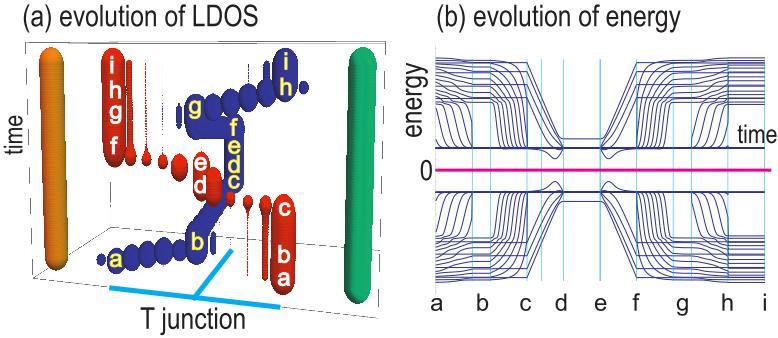
Figure 10: (a) Evolution of the LDOS as the two edges are braided across a trivial segment. (b) Evolution of the energy as a function of time. Each leg has ten sites. Alphabets a,b, $\cdots$, i denotes the steps (a), (b), $\cdots$, (i) of the braiding process in Fig.9. See also the caption of Fig.8.

IV.2 Braiding of two edges of a topological segment

We cannot braid two edges with the use of a single chain. This problem has been solved by employing a T-junctionAliceaBraid ; AA as shown in Fig.7. We consider a T-junction with three legs (named 1, 2, and 3) made of Kitaev chains. We set $\phi=0$ in all legs. Such a structure is designed in electric circuits as in Fig.12. We prepare the initial state [Fig.7(a)], which consists of the two horizontal legs 1 and 2 made topological and the vertical leg 3 made trivial. As we have already stated, it is possible to make a portion of a chain topological by controlling the chemical potential $\mu$ locally.

We braid two edges following the eight steps from (a) to (i) in the process as shown in Fig.7, where the initial and final states in Fig.7(a) and (i) are identical.

We explain the eight steps from (a) to (f) in the braiding of two edges of a topological segment in some details: See 7.

Two edge states emerge at the left and right hands of the horizontal line as indicated in Fig.7(a).

(1: a$\rightarrow$b) We move the edge on leg 2 toward the T-junction, by making the topological segment on leg 2 shorter. This process is done as explained in eq.(6) analytically.

(2: b$\rightarrow$c) When the edge reaches at the junction, we turn the trivial segment on leg 2 topological gradually so that the edge moves upward.

(3: c$\rightarrow$d) When leg 3 becomes topological entirely, we move the edge on leg 1 toward the T-junction.

(4: d$\rightarrow$e) When the edge reaches at the junction, we rotate the phase of leg 3 from $\phi_{\text{ini}}=0$ to $\phi_{\text{fin}}=\pi$. This process is done as explained in eq.(4) analytically.

(5: e$\rightarrow$f) When the phase of leg 3 becomes $\phi=\pi$, we move the edge right on leg 2.

(6: f$\rightarrow$g) When leg 2 becomes topological entirely, we move the edge on leg 3 downward.

(7: g$\rightarrow$h) When the edge on leg 3 reaches at the junction, we move it leftward on leg 1.

(8: h$\rightarrow$i) When leg 1 becomes topological entirely, we rotate the phase of the trivial segment on leg 3 from $\phi_{\text{ini}}=\pi$ to $\phi_{\text{fin}}=0$ on leg 3.

We present numerical results of this braiding process in Fig.8, which demonstrates that the process proceeds smoothly. It is confirmed that the energy of the edge states remains zero during the process and that the edge states are well separated from all other states as in Fig.8(b).

It is also confirmed that the Berry phase $\pi/4$ is acquired in the process (4: d $\rightarrow$ e) in Fig.8(b),

$$\Gamma_{\alpha\beta}(\text{d}\rightarrow\text{e})=\frac{\pi}{4}\delta_{\alpha\beta},$$ (39)

and it follows from (35) that

$$U_{\alpha\beta}(\text{d}\rightarrow\text{e})=e^{i\pi/4}\delta_{\alpha\beta},$$ (40)

where the phase of a topological segment is rotated from $\phi=0$ to $\phi=\pi$. There is no other contribution from the Berry phase.

There exists another contribution to the unitary transformation $U$ in Eq.(34), resulting from the fact that two states $\vec{\psi}_{A}$ and $\vec{\psi}_{B}$ are interchanged in the process (a$\rightarrow$i). The eigenfunctions (13) are explicitly given by

$$\vec{\psi}_{A}\left(0\right) =\frac{1}{\sqrt{2}}\left\{i,0,\cdots,0;-i,0,\cdots,0\right\},$$

$$\vec{\psi}_{B}\left(0\right) =\frac{1}{\sqrt{2}}\left\{0,\cdots,0,1;0,\cdots,0,1\right\},$$ (41)

at $\phi=0$, which are brought to

$$\vec{\psi}_{A}\left(\pi\right) =\frac{1}{\sqrt{2}}\left\{1,0,\cdots,0;1,0,\cdots,0\right\},$$

$$\vec{\psi}_{B}\left(\pi\right) =\frac{1}{\sqrt{2}}\left\{0,\cdots,0,-i;0,\cdots,0,i\right\},$$ (42)

at $\phi=\pi$. Thus, by the phase change ($\phi:0\rightarrow\pi$) at the step (4: d$\rightarrow$e) and by the interchange of the two edges, we obtain

$$\vec{\psi}_{A}\left(0\right)\rightarrow\vec{\psi}_{B}\left(0\right),\qquad\vec{\psi}_{B}\left(0\right)\rightarrow-\vec{\psi}_{A}\left(0\right).$$ (43)

On the other hand, the phase change ($\phi:\pi\rightarrow 0$) at the step (8: h$\rightarrow$i) does not affect the phases of the edge states. Combining these two effects, we obtain

$$i\sigma_{y}\left(\begin{array}[]{c}\vec{\psi}_{A}\left(0\right)\\ \vec{\psi}_{B}\left(0\right)\end{array}\right)=\left(\begin{array}[]{c}\vec{\psi}_{B}\left(0\right)\\ -\vec{\psi}_{A}\left(0\right)\end{array}\right).$$ (43)

Thus, the effect is summarized as the operation $i\sigma_{y}$.

The transformations (40) and (43) contribute to the diagonal and off-diagonal components of the unitary transformation (34). By combining these, the braiding is found to bring the initial state $(\vec{\psi}_{A},\vec{\psi}_{B})^{t}$ to the final state $U_{AB}(\vec{\psi}_{A},\vec{\psi}_{B})^{t}$ with

$$U_{AB}=\exp\left[\frac{i\pi}{4}\sigma_{y}\right]=\frac{1}{\sqrt{2}}\left(\begin{array}[]{cc}1&1\\ -1&1\end{array}\right).$$ (44)

The length of the legs can be as small as five sites since the penetration depth of a topological edge state is zero.

It is necessary to know how the braiding acts on the initial state $(\left|0\right\rangle,\left|1\right\rangle)$ in the qubit representation. Recall that the two sets of the states are related by Eq.(15). Hence, we find that the braiding operation $U_{12}$ acts on the one-qubit state as

$$U_{12}\left(\begin{array}[]{c}\vec{\psi}_{|0\rangle}\\ \vec{\psi}_{|1\rangle}\end{array}\right) =U_{\text{basis}}U_{AB}U_{\text{basis}}^{-1}\left(\begin{array}[]{c}\vec{\psi}_{A}\\ \vec{\psi}_{B}\end{array}\right)$$ (49)

$$=\left(\begin{array}[]{cc}e^{-i\pi/4}&0\\ 0&e^{i\pi/4}\end{array}\right)\left(\begin{array}[]{c}\vec{\psi}_{|0\rangle}\\ \vec{\psi}_{|1\rangle}\end{array}\right),$$ (54)

or

$$U_{12}\left(\begin{array}[]{c}\left|0\right\rangle\\ \left|1\right\rangle\end{array}\right)=\left(\begin{array}[]{cc}e^{-i\pi/4}&0\\ 0&e^{i\pi/4}\end{array}\right)\left(\begin{array}[]{c}\left|0\right\rangle\\ \left|1\right\rangle\end{array}\right).$$ (55)

The braiding process acts as a phase-shift gate in the qubit representation. It follows that

$$U_{12}^{2}=-i\sigma_{z},$$ (56)

and hence $U_{12}$ is proportional to the square root of the Z gate,

$$U_{12}=\sqrt{-i}\sqrt{\sigma_{z}},$$ (57)

which is the $\sqrt{\sigma_{Z}}$ gateLes .

IV.3 Braiding of two edges of a trivial segment

We discuss the braiding of two edges of a trivial segment. The braiding process is similar to the previous case: It occurs following nine steps from (a) to (i), as illustrated in Fig.9. A new configuration is Fig.9(d), where all three legs are topological. It is understood that the point at the junction is the edge of the vertical topological segment. A phase rotation by $\pi$ occurs on a topological segment from Fig.9(d) to (e) with a contributing to the Berry phase, and on a trivial segment from Fig.9(h) to (i) with no contribution to the Berry phase. We show numerical results of this braiding process in Fig.10, which demonstrates that the process proceeds smoothly.

It is convenient to relabel the edge states as

$$(\vec{\psi}_{A}^{1},\vec{\psi}_{B}^{1},\vec{\psi}_{A}^{2},\vec{\psi}_{B}^{2},\cdots)\rightarrow(\vec{\psi}_{1},\vec{\psi}_{2},\vec{\psi}_{3},\vec{\psi}_{4},\cdots),$$ (58)

as shown in Fig.1. The braiding process involves two topological segments, and hence it is a two-qubit operation. The two-qubit basis is $\left|n_{1}n_{2}\right\rangle$ as given by Eq.(18), the first qubit $n_{1}$ is formed by $\vec{\psi}_{1}$ and $\vec{\psi}_{2}$, while the second qubit $n_{2}$ is formed by $\vec{\psi}_{3}$ and $\vec{\psi}_{4}$.

However, since the braiding occurs for a pair $\vec{\psi}_{2}$ and $\vec{\psi}_{3}$, it is convenient to consider two qubits $(\vec{\psi}_{2},\vec{\psi}_{3})$ and $(\vec{\psi}_{1},\vec{\psi}_{4})$. Hence, we introduce a new two-qubit basis $|n_{+}n_{-}\}$, where $n_{+}=0,1$ is a qubit formed by $\vec{\psi}_{2}$ and $\vec{\psi}_{3}$, while $n_{-}=0,1$ is a qubit formed by $\vec{\psi}_{1}$ and $\vec{\psi}_{4}$.The transformation is given by the fusion matrix of the Ising anyonPachos ; Stanes ; Aasen ,

$$\left(\begin{array}[]{c}|00\}\\ |11\}\\ |01\}\\ |10\}\end{array}\right)=\frac{1}{\sqrt{2}}\left(\begin{array}[]{cccc}1&1&0&0\\ -1&1&0&0\\ 0&0&1&1\\ 0&0&-1&1\end{array}\right)\left(\begin{array}[]{c}\left|00\right\rangle\\ \left|11\right\rangle\\ \left|01\right\rangle\\ \left|10\right\rangle\end{array}\right).$$ (59)

The inverse relation reads

$$\left(\begin{array}[]{c}\left|00\right\rangle\\ \left|11\right\rangle\\ \left|01\right\rangle\\ \left|10\right\rangle\end{array}\right)=\frac{1}{\sqrt{2}}\left(\begin{array}[]{cccc}1&-1&0&0\\ 1&1&0&0\\ 0&0&1&-1\\ 0&0&1&1\end{array}\right)\left(\begin{array}[]{c}|00\}\\ |11\}\\ |01\}\\ |10\}\end{array}\right).$$ (60)

Here, we recall that the formula (55) acts on $\left|0\right\rangle$ and $\left|1\right\rangle$ for the exchange of $\vec{\psi}_{1}$ and $\vec{\psi}_{2}$. Now, the corresponding exchange operator is $U_{23}$ for the exchange of $\vec{\psi}_{2}$ and $\vec{\psi}_{3}$. Since it acts on $|0n_{-}\}$ and $|1n_{-}\}$ irrespective of the second component $n_{-}$, we obtain

$$U_{23}\left(\begin{array}[]{c}|00\}\\ |11\}\end{array}\right)=\left(\begin{array}[]{cc}e^{-i\pi/4}&0\\ 0&e^{i\pi/4}\end{array}\right)\left(\begin{array}[]{c}|00\}\\ |11\}\end{array}\right),$$ (61)

and

$$U_{23}\left(\begin{array}[]{c}|01\}\\ |10\}\end{array}\right)=\left(\begin{array}[]{cc}e^{-i\pi/4}&0\\ 0&e^{i\pi/4}\end{array}\right)\left(\begin{array}[]{c}|01\}\\ |10\}\end{array}\right).$$ (62)

Then, we determine how $U_{23}$ acts on the original basis. We use Eq.(60) to find

$$U_{23}\left|00\right\rangle=\frac{1}{\sqrt{2}}\left(U_{23}|00\}-U_{23}|11\}\right).$$ (63)

Then, we use Eq.(61) to derive

$$U_{23}\left|00\right\rangle=\frac{1}{\sqrt{2}}\left(e^{-i\pi/4}|00\}-e^{i\pi/4}|11\}\right).$$ (64)

Finally, we use Eq.(59) to find

$$U_{23}\left|00\right\rangle=\frac{1}{\sqrt{2}}\left(\left|00\right\rangle-i\left|11\right\rangle\right).$$ (65)

We may carry out similar analysis for $U_{23}\left|11\right\rangle$, $U_{23}\left|01\right\rangle$ and $U_{23}\left|10\right\rangle$. The results are summarized as

$$U_{23}\left(\begin{array}[]{c}\left|00\right\rangle\\ \left|01\right\rangle\\ \left|10\right\rangle\\ \left|11\right\rangle\end{array}\right)=\frac{1}{\sqrt{2}}\left(\begin{array}[]{cccc}1&0&0&-i\\ 0&1&-i&0\\ 0&-i&1&0\\ -i&0&0&1\end{array}\right)\left(\begin{array}[]{c}\left|00\right\rangle\\ \left|01\right\rangle\\ \left|10\right\rangle\\ \left|11\right\rangle\end{array}\right).$$ (66)

Since the parity is preserved during the braiding process, it can be decomposed into the even parity

$$U_{23}\left(\begin{array}[]{c}\left|00\right\rangle\\ \left|11\right\rangle\end{array}\right)=\frac{1}{\sqrt{2}}\left(\begin{array}[]{cc}1&-i\\ -i&1\end{array}\right)\left(\begin{array}[]{c}\left|00\right\rangle\\ \left|11\right\rangle\end{array}\right),$$ (67)

and the odd parity

$$U_{23}\left(\begin{array}[]{c}\left|01\right\rangle\\ \left|10\right\rangle\end{array}\right)=\frac{1}{\sqrt{2}}\left(\begin{array}[]{cc}1&-i\\ -i&1\end{array}\right)\left(\begin{array}[]{c}\left|01\right\rangle\\ \left|10\right\rangle\end{array}\right).$$ (68)

It follows that

$$U_{23}^{2}=-i\sigma_{x}.$$ (69)

The operation is a square root of the NOT gate, that is the $\sqrt{\sigma_{X}}$ gateLes ,

$$U_{23}=\sqrt{-i}\sqrt{\sigma_{x}}.$$ (70)

These results are exactly the same as those in the two-qubit operation based on Majorana fermionsIvanov .

IV.4 Entangled states

We show that an entangle state is generated by a two-qubit operation. For example, we have

$$U_{23}\left|00\right\rangle=\left|00\right\rangle-i\left|11\right\rangle.$$ (71)

This is an entangled state. Let us prove it. If it is not, the final state should be a pure state and written as

$$U_{23}\left|00\right\rangle =\left(\alpha_{1}\left|0\right\rangle+\beta_{1}\left|1\right\rangle\right)\otimes\left(\alpha_{2}\left|0\right\rangle+\beta_{2}\left|1\right\rangle\right)$$

$$=\alpha_{1}\alpha_{2}\left|00\right\rangle+\alpha_{1}\beta_{2}\left|01\right\rangle+\beta_{1}\alpha_{2}\left|10\right\rangle+\beta_{1}\beta_{2}\left|11\right\rangle.$$ (72)

It follows from Eq.(71) that $\alpha_{1}\alpha_{2}\neq 0$ and $\beta_{1}\beta_{2}\neq 0$, and hence $\alpha_{1}\alpha_{2}\beta_{1}\beta_{2}\neq 0$, which yields $\alpha_{1}\beta_{2}\neq 0$ and $\beta_{1}\alpha_{2}\neq 0$. This contradicts Eq.(71). Namely, an entangled state is produced by a braiding of two edge solitons across a trivial segment.

IV.5 Braiding relations

We explore the braiding relations. We have explicitly constructed $U_{12}$ and $U_{23}$. It is obvious that $U_{2j-1,2j}$ and $U_{2j,2j+1}$ have the same expressions as these, for $j=1,2,3,\cdots$. By using the matrix representation of these braiding operations, we can check that

$$U_{j-1,j}U_{j,j+1}U_{j-1,j}=U_{j,j+1}U_{j-1,j}U_{j,j+1},$$

$$U_{j,j+1}U_{j^{\prime},j^{\prime}+1}=U_{j^{\prime},j^{\prime}+1}U_{j,j+1}\quad\text{for}\quad\left|j-j^{\prime}\right|\geq 2,$$

$$U_{j-1,j}U_{j,j+1}\neq U_{j,j+1}U_{j-1,j},$$ (73)

which are the braiding relationsIvanov .

IV.6 Clifford gates

We have constructed the $\sqrt{\sigma_{X}}$ and $\sqrt{\sigma_{Z}}$ gates in Eq.(70) and Eq.(57), respectively. The $\sqrt{\sigma_{Y}}$ gate is constructed by their successive operations as

$$\sqrt{\sigma_{Y}}=\sqrt{i}\sqrt{\sigma_{X}}\sqrt{\sigma_{Z}}=\frac{1}{\sqrt{-i}}U_{23}U_{12}.$$ (74)

These sets construct the Pauli gates. On the other hand, the Hadamard gate is constructed byLes

$$iU_{12}U_{23}U_{12}=iU_{23}U_{12}U_{23}=\frac{1}{\sqrt{2}}\left(\begin{array}[]{cccc}1&0&0&1\\ 0&-1&1&0\\ 0&1&1&0\\ 1&0&0&-1\end{array}\right),$$ (75)

because the set of $\left|00\right\rangle$ and $\left|11\right\rangle$ and the set of $\left|01\right\rangle$ and $\left|10\right\rangle$ are independent in the braiding operation.

IV.7 Readout of unitary gate operation

We have explained in Subsec. II.4 how we can initialize the qubit states to the pure state $\left|00\cdots 0\right\rangle$. Various qubit states are generated by operating various unitary gate operations. The key role is played by the Berry phase in the process of braiding, which utilizes the gauge degree of freedom. Since the external current freezes the gauge degree of freedom, the braiding process should be carried out in the absence of the external current. We have explained in Subsec. III.3 that we can store (read) the qubit information in (from) the LC resonators by manipulating (measuring) the voltages at the edge states even in such a circumstance.

In this subsection, we argue how the qubit information stored in the LC resonators changes by a unitary gate operation. One qubit states are $\left|0\right\rangle$ and $\left|1\right\rangle$. The state $\left|0\right\rangle$ ($\left|1\right\rangle$) is created by applying the same (opposite) voltage at the two edges of one topological segment simultaneously. After the application of the voltage, the in-phase (opposite) voltage-current oscillation starts in a set of LC resonators, which represent the state $\left|0\right\rangle$ ($\left|1\right\rangle$).

We discuss the one-qubit gate operation associated with the braiding of the two edge states across a topological segment, which is represented by the one-qubit unitary operator (55), or

$$U_{12}|0\rangle\mapsto e^{-i\pi/4}|0\rangle,\qquad U_{12}|1\rangle\mapsto e^{i\pi/4}|1\rangle.$$ (76)

These results are observed electrically as a phase shift in the voltage at the two edge states on the capacitor channel,

$$(e^{i\omega_{0}t},e^{i\omega_{0}t})\mapsto(e^{i\omega_{0}t-i\pi/4},e^{i\omega_{0}t-i\pi/4})$$ (77)

for $U_{12}|0\rangle$, and

$$(e^{i\omega_{0}t},-e^{i\omega_{0}t})\mapsto(e^{i\omega_{0}t+i\pi/4},-e^{i\omega_{0}t+i\pi/4})$$ (78)

for $U_{12}|1\rangle$.

We may similarly discuss the two-qubit operation associated with the braiding of the two edge states across a trivial segment. The actual braiding is represented by the one-qubit unitary operator (66), or

$$U_{23}|00\rangle\mapsto\frac{1}{\sqrt{2}}\left(00\rangle-i\left|11\right\rangle\right).$$ (79)

The result of the operation $U_{23}$ on the state $|00\rangle$ is observed electrically as a phase shift in the voltage at the four edge states on the capacitor channel,

$$(e^{i\omega_{0}t},e^{i\omega_{0}t};e^{i\omega_{0}t},e^{i\omega_{0}t})$$

$$\quad\mapsto\frac{1}{\sqrt{2}}(e^{i\omega_{0}t},e^{i\omega_{0}t};e^{i\omega_{0}t},e^{i\omega_{0}t})$$

$$\quad\quad\quad\quad-\frac{i}{\sqrt{2}}(e^{i\omega_{0}t},-e^{i\omega_{0}t};e^{i\omega_{0}t},-e^{i\omega_{0}t})$$

$$=(e^{i\omega_{0}t-i\pi/4},e^{i\omega_{0}t+i\pi/4};e^{i\omega_{0}t-i\pi/4},e^{i\omega_{0}t+i\pi/4}).$$ (80)

Similar results are obtained for the other states. In general, the change of phase shift is registered in a set of LC resonators in any gate processing. We can read the qubit information by measuring the phase shifts from a set of resonators after all braidings are over.

V Creation and annihilation of edge solitons

We have derived the basic formulas familiar in topological quantum computations by calculating the Berry phase with the use of T-junction geometry in the electric-circuit formalism. It is interesting to reformulate our scheme to know to what extent we can simulate the standard Majorana-operator formalism by the electric-circuit formalism.

A topological edge state emerges at the boundary between the topological and trivial segments of a Kitaev chain and is observable as an impedance peak in electric circuit. Such a state is interpreted as a topological soliton because it is a localized particle-like object and has a topological stability by intertwining the topological and the trivial segments. We call it an edge soliton when we focus on the aspect of soliton. An edge soliton in the present model is quite similar to a sine-Gordon soliton in the sine-Gordon model. Exchange statistic of topological solitons is intriguing: A topological soliton in the classical sine-Gordon model has been arguedColeman ; Mandel to be a Thirring fermionThirring . Similarly, we now argue that an edge soliton in the Kitaev model behaves as a Majorana-fermion because the circuit contains the capacitor channel and the inductor channel corresponding to the electron band and the hole band.

We have obtained two zero-energy solutions (13), where $\vec{\psi}_{A}$ and $\vec{\psi}_{B}$ are perfectly localized at the left edge and the right edge of a topological segment, respectively. They describe a pair of edge solitons. As we have remarked in Eq.(22), the Kitaev Hamiltonian is equivalent to the circuit Laplacian. The two systems are equivalent at the Hamiltonian level, and there is one-to-one correspondence between the wave functions in these two systems. The wave function is the voltage function (24) in electric circuits. Edge solitons are materialized as impedance peaks in the electric circuit: See Figs.4 and 5.

Here, let us summarize key features of edge solitons.

(i) We start with the electric circuit with all TCUs being off, which describes the Kitaev chain in the trivial phase.

(ii) We create $N$ topological segments together with $N$ pairs of edge solitons by switching on the TCUs attached to those segments.

(ii) A pair of edge solitons are observable by peaks in voltage or impedance both in the capacitor channel and the inductor channel: See Fig.5(c).

(iii) Two edge solitons cannot occupy a single site, which means that they are subject to the exclusion principle.

(iv) We may move an edge freely by expanding or shrinking a topological segment by switching on or off TCUs, which means that we can flit an edge soliton from one site to a neighboring site.

These properties of edge solitons allow us to introduce a creation operator of one edge soliton. The wave function $\vec{\psi}_{A}$ in Eqs.(13) implies that one edge soliton has a component with phase $ie^{-i\phi/2}$ in the electron sector and a portion of phase $-ie^{i\phi/2}$ in the hole sector at $x=0$. It describes a creation of an impedance peak carrying the corresponding phases in the capacitor channel and the inductor channel at site $x=0$. A similar creation operator is introduced with respect to the edge soliton with the wave function $\vec{\psi}_{B}$ at $x=m$.

V.1 One topological segment

Since an appropriately designed electric circuit is equivalent to the Kitaev model at the Hamiltonian level, we may reformulate such an electric circuit as a lattice model. We recall that an edge soliton is observable as an impedance peak, which consists of two parts in the capacitor channel and inductor channel as in Fig.5(c). Let us define the creation operator of an edge soliton with phase $\phi=0$ in the capacitor (inductor) channel at $x$ by $a_{x}^{\dagger}$ ($b_{x}^{\dagger}$). It must be that $a_{x}^{\dagger 2}=b_{x}^{\dagger 2}=0$ due to the exclusion principle imposed on the edge soliton in each channel.

We then define the creation operators $\gamma_{A}^{\dagger}$ and $\gamma_{B}^{\dagger}$ of the edge solitons with phase $\phi$ by

$$\gamma_{A}^{\dagger} =\sqrt{2}\vec{a}^{\dagger}\cdot\vec{\psi}_{A}=ie^{-i\phi/2}a_{0}^{\dagger}-ie^{i\phi/2}b_{0}^{\dagger},$$

$$\gamma_{B}^{\dagger} =\sqrt{2}\vec{a}^{\dagger}\cdot\vec{\psi}_{B}=e^{-i\phi/2}a_{m}^{\dagger}+e^{i\phi/2}b_{m}^{\dagger},$$ (81)

where $\vec{\psi}_{A}$ and $\vec{\psi}_{B}$ are the wave functions given by Eqs.(13), and

$$\vec{a}^{\dagger}=(a_{0}^{\dagger},a_{1}^{\dagger},\cdots,a_{m}^{\dagger};b_{0}^{\dagger},b_{1}^{\dagger},\cdots,b_{m}^{\dagger}).$$ (82)

Although it appears that $\gamma_{A}$ is composed of $2(m+1)$ independent components, this is not the case. The electric circuit is designed to simulate the Kitaev model (3) precisely at the Hamiltonian level, which originally contains the same information in the electron sector and the hole sector related via complex conjugation. Indeed, the wave functions $\vec{\psi}_{A}$ and $\vec{\psi}_{B}$ described by Eqs.(13) have this property. Consequently it should be that $b_{j}^{\dagger}=a_{j}$, or

$$\vec{a}^{\dagger}=(a_{0}^{\dagger},a_{1}^{\dagger},\cdots,a_{m}^{\dagger};a_{0},a_{1},\cdots,a_{m}).$$ (83)

Then, it follows from Eqs.(81) that $\gamma_{A}=\gamma_{A}^{\dagger}$ and $\gamma_{B}=\gamma_{B}^{\dagger}$. We rewrite Eqs.(81) as

$$\gamma_{A} =ie^{-i\phi/2}a_{0}^{\dagger}-ie^{i\phi/2}a_{0},$$

$$\gamma_{B} =e^{-i\phi/2}a_{m}^{\dagger}+e^{i\phi/2}a_{m}.$$ (84)

Now, the exclusion principle indicates that there are only two states at one site, i.e., whether an edge soliton is absent or present at one site, which we denote $|0\rangle\!\rangle$ and $|1\rangle\!\rangle$, with $a_{x}^{\dagger}|0\rangle\!\rangle=|1\rangle\!\rangle$ and $a_{x}|1\rangle\!\rangle=|0\rangle\!\rangle$. In the matrix form, these relations are written in the form of

$$a_{x}^{\dagger}\left(\begin{array}[]{c}|0\rangle\!\rangle\\ |1\rangle\!\rangle\end{array}\right) =\left(\begin{array}[]{cc}0&1\\ 0&0\end{array}\right)\left(\begin{array}[]{c}|0\rangle\!\rangle\\ |1\rangle\!\rangle\end{array}\right),$$ (91)

$$a_{x}\left(\begin{array}[]{c}|0\rangle\!\rangle\\ |1\rangle\!\rangle\end{array}\right) =\left(\begin{array}[]{cc}0&0\\ 1&0\end{array}\right)\left(\begin{array}[]{c}|0\rangle\!\rangle\\ |1\rangle\!\rangle\end{array}\right),$$ (98)

which lead to

$$a_{x}^{\dagger}=\left(\begin{array}[]{cc}0&1\\ 0&0\end{array}\right),\qquad a_{x}=\left(\begin{array}[]{cc}0&0\\ 1&0\end{array}\right).$$ (99)

We obtain the anticommutation relation, $a_{x}a_{x}^{\dagger}+a_{x}^{\dagger}a_{x}=1$, for an edge soliton in each channel, showing that it behaves as a fermion. Consequently, we obtain $\gamma_{A}^{2}=\gamma_{B}^{2}=1$.

However, we have no information on the commutation relation between $\gamma_{A}$ and $\gamma_{B}$, which is the exchange statistics of edge solitons.

V.2 Many topological segments

We next study a Kitaev chain containing $N$ topological segments. For definiteness each topological (trivial) segment is assumed to be made of $m+1$ ($m-1$) sites, as in Fig.1. The $j$-th topological segment produces two topological edge states $\vec{\psi}_{A}^{j}$ and $\vec{\psi}_{B}^{j}$ given by Eqs.(13). Then, we may introduce a set of the operators as

$$\gamma_{A}^{j}=\sqrt{2}\vec{a}_{j}^{\dagger}\cdot\vec{\psi}_{A},\qquad\gamma_{B}^{j}=\sqrt{2}\vec{a}_{j}^{\dagger}\cdot\vec{\psi}_{B}$$ (100)

with

$$\vec{a}_{j}^{\dagger}=(a_{j^{\prime}}^{\dagger},a_{j^{\prime}+1}^{\dagger},\cdots,a_{j^{\prime}+m}^{\dagger};a_{j^{\prime}},a_{j^{\prime}+1},\cdots,a_{j^{\prime}+m}),$$ (101)

where $j^{\prime}=(2j-2)m$.

It may be convenient to relabel the edge states as

$$(\gamma_{A}^{1},\gamma_{B}^{1},\gamma_{A}^{2},\gamma_{B}^{2},\cdots)\rightarrow(\gamma_{1},\gamma_{2},\gamma_{3},\gamma_{4},\cdots)$$ (102)

in accord with Eq.(58). Then, it follows from the above arguments that

$$(\gamma_{j})^{2}=1,$$ (103)

for any $j$, because any edge soliton has components both in the electron sector and the hole sector, and each component is subject to the exclusion principle. We shall see that $\gamma_{j}$ is the Majorana operator in the succeeding section.

VI Exchange statistics

We investigate the exchange statistics of edge solitons. We have already studied the way and the result of exchanging two edge states by calculating the Berry phase with the use of T-junction geometry in Sec. IV. Here we reanalyze the problem in terms of edge soliton operators. We consider a T-junction with three legs (named 1, 2, and 3) made of Kitaev chains as shown in Fig.7 and Fig.9. We set $\phi=0$ in all legs.

VI.1 Braiding of two edges across a topological segment

We braid two edge solitons across a topological segment, following the eight steps from (a) to (i) in Fig.7, which we have studied in Subsec. IV.2. We examine how these processes affect the edge solitons at $x=1$ and $x=m$. There are two effects. (i) If the edge soliton $\gamma_{A}$ ($\gamma_{B}$) at $x=0$ ($m$) were brought to $x=m$ ($0$) without changing the "superconducting phase" $\phi$, we would have

$$\gamma_{A} =ia_{0}^{\dagger}-ia_{0}\rightarrow ia_{m}^{\dagger}-ia_{m},$$

$$\gamma_{B} =a_{m}^{\dagger}+a_{m}\rightarrow a_{0}^{\dagger}+a_{0},$$ (104)

by setting $\phi=0$ in Eqs.(84), and then by exchanging the indices $0$ and $m$. (ii) Actually, by the phase change at the step (4: d$\rightarrow$e), the eigenfunctions (13) read

$$\gamma_{A}=a_{0}^{\dagger}+a_{0},\qquad\gamma_{B}=-ia_{m}^{\dagger}+ia_{m},$$ (105)

by setting $\phi=\pi$ in Eqs.(84). Note that the phase change at the step (8: h$\rightarrow$i) does not affect the edge solitons. Combining these two effects, we obtain

$$\gamma_{A}\rightarrow-\gamma_{B},\qquad\gamma_{B}=\gamma_{A},$$ (106)

or

$$\gamma_{A}\gamma_{B}\rightarrow-\gamma_{B}\gamma_{A}.$$ (107)

This is the result of a single exchange of two edge solitons in a topological segment. A double exchange implies $\gamma_{A}\rightarrow-\gamma_{A}$, $\gamma_{B}=-\gamma_{B}$, as expected. An edge soliton is an Ising anyon.

VI.2 Braiding of two edges across a trivial segment

We discuss the braiding of two edge solitons across a trivial segment, following the eight steps from (a) to (i) in Fig.9, which we have studied in Subsec. IV.3. We examine how these processes affect the edge solitons at $x=m$ and $x=2m$. A phase rotation by $\pi$ occurs on a topological segment from Fig.9(d) to (e) with a contributing to the wave function, and on a trivial segment from Fig.9(h) to (i) with no contribution.

We examine how these processes affect the edge solitons. For definiteness we study the exchange of $\gamma_{B}^{1}$ and $\gamma_{A}^{2}$ in Fig.1, or

$$\gamma_{B}^{1} =e^{-i\phi/2}a_{m}^{\dagger}+e^{i\phi/2}a_{m}=\sqrt{2}\vec{a}_{1}^{\dagger}\cdot\vec{\psi}_{B},$$

$$\gamma_{A}^{2} =ie^{-i\phi/2}a_{2m}^{\dagger}-ie^{i\phi/2}a_{2m}=\sqrt{2}\vec{a}_{2}^{\dagger}\cdot\vec{\psi}_{A},$$ (108)

with

$$\vec{a}_{1}^{\dagger} =(a_{0}^{\dagger},a_{1}^{\dagger},\cdots,a_{m}^{\dagger};a_{0},a_{1},\cdots,a_{m}),$$

$$\vec{a}_{2}^{\dagger} =(a_{2m}^{\dagger},a_{2m+1}^{\dagger},\cdots,a_{3m}^{\dagger};a_{2m},a_{2m+1},\cdots,a_{3m}).$$ (109)

There are two effects. (i) The edge soliton $\gamma_{B}^{1}$ ($\gamma_{A}^{2}$) at $x=m$ ($2m$) is brought to $x=2m$ ($m$), which results in

$$\gamma_{B}^{1} =a_{m}^{\dagger}+a_{m}\rightarrow a_{2m}^{\dagger}+a_{2m},$$

$$\gamma_{A}^{2} =ia_{2m}^{\dagger}-ia_{2m}\rightarrow ia_{m}^{\dagger}-ia_{m},$$ (110)

by setting $\phi=0$ in Eqs.(108), and then by exchanging indices $m$ and $2m$. (ii) By the phase change at the step (4: d$\rightarrow$e), the eigenfunctions (13) read

$$\gamma_{B}^{1}=-ia_{m}^{\dagger}+ia_{m},\qquad\gamma_{A}^{2}=a_{2m}^{\dagger}+a_{2m},$$ (111)

by setting $\phi=\pi$ in Eqs.(84). Note that the phase change at the step (8: h$\rightarrow$i) does not affect the edge solitons. Combining these two effects, we obtain

$$\gamma_{B}^{1}\rightarrow-\gamma_{A}^{2},\qquad\gamma_{A}^{2}\rightarrow\gamma_{B}^{1},$$ (112)

or

$$\gamma_{B}^{1}\gamma_{A}^{2}\rightarrow-\gamma_{A}^{2}\gamma_{B}^{1}.$$ (113)

This is the result of a single exchange of two edge solitons across a topological segment.

VI.3 Braiding operators

When we label the edge solitons as in Eq.(102), we obtain from Eq.(107) and Eq.(113) that $\gamma_{j}\gamma_{j+1}=-\gamma^{j+1}\gamma_{j}$. By repeating the exchange of adjacent edge solitons, it is possible to generalize this result to $\gamma_{i}\gamma_{j}=-\gamma_{j}\gamma_{i}$, which we combine with Eq.(103) to obtain

$$\gamma_{i}\gamma_{j}+\gamma_{j}\gamma_{i}=2\delta_{ij}$$ (114)

for any $i$ and $j$. Furthermore, the braiding results (106) and (112) are generalized to the braiding operations

$$U_{ij}:\gamma_{i}\rightarrow-\gamma_{j},\qquad U_{ij}:\gamma_{j}\rightarrow\gamma_{i},$$ (115)

or

$$U_{ij}\gamma_{i}U_{ij}^{-1}=\gamma_{j},\qquad U_{ij}\gamma_{j}U_{ij}^{-1}=-\gamma_{i}.$$ (116)

Hence, the braiding operator is given by

$$U_{ij}=\frac{1}{\sqrt{2}}(1+\gamma_{j}\gamma_{i})=\exp[\pi\gamma_{j}\gamma_{i}/4],$$ (117)

as agrees with the standard resultIvanov .

VI.4 Qubits in operator formalism

VI.4.1 One-qubit state

We have associated the operators $\gamma_{A}$ and $\gamma_{B}$ to the edge solitons so that they create the wave functions $\vec{\psi}_{A}$ and $\vec{\psi}_{B}$ given by Eqs.(13). Similarly, we may associate the operators $f$ and $f^{{}^{\dagger}}$ to the states described by the wave functions $\vec{\psi}_{|0\rangle}$ and $\vec{\psi}_{|1\rangle}$ as

$$f =\vec{a}^{\dagger}\cdot\vec{\psi}_{|0\rangle}=(\gamma_{A}+i\gamma_{B})/2,$$

$$f^{\dagger} =\vec{a}^{\dagger}\cdot\vec{\psi}_{|1\rangle}=(\gamma_{A}-i\gamma_{B})/2,$$ (118)

where $\vec{a}^{\dagger}$ is defined by Eq.(83). We then have

$$\gamma_{A}=f+f^{\dagger},\qquad\gamma_{B}=i(f^{\dagger}-f).$$ (119)

The one-qubit states, $|0\rangle$ and $|1\rangle$, are defined as the empty and the occupied states with respect to fermion operator $f$,

$$f|0\rangle=0,\quad f^{\dagger}|1\rangle=0,\quad f^{\dagger}|0\rangle=|1\rangle,\quad f|1\rangle=|0\rangle.$$ (120)

The set of states $\left|0\right\rangle$ and $\left|1\right\rangle$ constitutes one qubit for application to topological quantum computers.

We recall that the braiding of two edge solitons across a topological segment is given by $U_{12}=(1+\gamma^{2}\gamma^{1})/\sqrt{2}$ as in Eq.(117), or

$$U_{12}=\frac{1}{\sqrt{2}}[1+i(f_{1}^{\dagger}-f_{1})(f_{1}+f_{1}^{\dagger})].$$ (121)

By operating this to one-qubit states, we find

$$U_{12}\left|0\right\rangle=\frac{1}{\sqrt{2}}(1-i)\left|0\right\rangle,\qquad U_{12}\left|1\right\rangle=\frac{1}{\sqrt{2}}(1+i)\left|1\right\rangle.$$ (122)

Hence, we obtain

$$U_{12}\left(\begin{array}[]{c}\left|0\right\rangle\\ \left|1\right\rangle\end{array}\right)=\left(\begin{array}[]{cc}e^{-i\pi/4}&0\\ 0&e^{i\pi/4}\end{array}\right)\left(\begin{array}[]{c}\left|0\right\rangle\\ \left|1\right\rangle\end{array}\right),$$ (123)

which is nothing but Eq.(55).

VI.4.2 Multi-qubit state

One-qubit states $\left|0\right\rangle_{j}$ and $\left|1\right\rangle_{j}$ are similarly constructed for the $j$-th topological segment with the use of

$$f_{j}=(\gamma_{A}^{j}+i\gamma_{B}^{j})/2,\quad f_{j}^{\dagger}=(\gamma_{A}^{j}-i\gamma_{B}^{j})/2,$$ (124)

as in Eq.(120), or

$$f_{j}|1\rangle_{j}=|0\rangle_{j},\qquad f_{j}^{\dagger}|0\rangle_{j}=|1\rangle_{j}.$$ (125)

Two-qubit states are defined by

$$f_{1}|00\rangle=f_{2}|00\rangle=f_{1}^{{\dagger}}|11\rangle=f_{2}^{{\dagger}}|11\rangle=0,$$

$$|10\rangle=f_{1}^{{\dagger}}|00\rangle,\quad|01\rangle=f_{2}^{{\dagger}}|00\rangle,\quad|11\rangle=f_{1}^{{\dagger}}f_{2}^{{\dagger}}|00\rangle.$$ (126)

The many-body states are given by the direct product,

$$\left|n_{1}n_{2}\cdots n_{N}\right\rangle=\left|n_{1}\right\rangle_{1}\otimes\left|n_{2}\right\rangle_{2}\otimes\cdots\otimes\left|n_{N}\right\rangle_{N}$$ (127)

with $n_{j}=0,1$.

We study the two-qubit states some in detail. The braiding across a trivial segment is given by $U_{23}=(1+\gamma^{3}\gamma^{2})/\sqrt{2}$ as in Eq.(117), or

$$U_{23}=\frac{1}{\sqrt{2}}[1+i(f_{2}+f_{2}^{\dagger})(f_{1}^{\dagger}-f_{1})].$$ (128)

By operating this to one-qubit states, we find

$$U_{23}\left(\begin{array}[]{c}\left|00\right\rangle\\ \left|01\right\rangle\\ \left|10\right\rangle\\ \left|11\right\rangle\end{array}\right)=\frac{1}{\sqrt{2}}\left(\begin{array}[]{cccc}1&0&0&-i\\ 0&1&-i&0\\ 0&-i&1&0\\ -i&0&0&1\end{array}\right)\left(\begin{array}[]{c}\left|00\right\rangle\\ \left|01\right\rangle\\ \left|10\right\rangle\\ \left|11\right\rangle\end{array}\right),$$ (129)

which is nothing but Eq.(66).

VII Electric-circuit realization (revisited)

We have explained how to simulate the Kitaev chain by an electric circuit in Sec. III. In this section we construct the circuit Laplacians explicitly for the topological and trivial phases.

VII.1 Topological and trivial phases

The Kirchhoff current law (20) is summarized as Eq.(21), or

$$I_{a}\left(\omega\right)=\sum_{b}J_{ab}\left(\omega\right)V_{b}\left(\omega\right),$$ (130)

where the circuit Laplacian $J_{ab}\left(\omega\right)$ is expressed as

$$J=\left(\begin{array}[]{cc}h_{1}&g_{1}\\ g_{2}&h_{2}\end{array}\right).$$ (131)

We study $J_{ab}$ explicitly in what follows.

We first study the circuit given in the right-hand side of Fig.3(b). We shall show that it describes the topological phase. Analyzing the Kirchhoff current law for the circuit, we obtainEzawaMajo

$$h_{1} =-2C\cos k+2C-(\omega^{2}L_{0})^{-1},$$

$$h_{2} =2(\omega^{2}L)^{-1}\cos k-2(\omega^{2}L)^{-1}+C_{0},$$ (132)

and

$$g_{1} =-C_{X}e^{ik}+(\omega^{2}L_{X})^{-1}e^{-ik},$$

$$g_{2} =(\omega^{2}L_{X})^{-1}e^{ik}-C_{X}e^{-ik}.$$ (133)

We make the following observation. (i) Capacitors and inductors on the main two channels appear in the diagonal elements $h_{1}$ and $h_{2}$. (ii) Those attached to the ground appear also appear in $h_{1}$ and $h_{2}$. (iii) Those in the pairing interactions appear in the off-diagonal elements $g_{1}$ and $g_{2}$.

In identifying the circuit Laplacian with the Kitaev Hamiltonian as in Eq.(22), it is necessary to require

$$\omega_{0}\equiv 1/\sqrt{LC}=1/\sqrt{L_{0}C_{0}}=1/\sqrt{L_{X}C_{X}}$$ (134)

for PHS to hold for the circuit. At $\omega=\omega_{0}$, the circuit Laplacian (131) is reduced to

$$J=\left[2C(1-\cos k)-C_{0}\right]\sigma_{z}+2C_{X}\sigma_{y}\sin k.$$ (135)

It follows from Eq.(22) that

$$t=-C,\quad\mu=-2C+C_{0},\quad\Delta=C_{X}.$$ (136)

The parameters charactering the Kitaev model (3) are determined by these equations in terms of electric elements for the right-hand side of Fig.3(b). The system is topological since $\left|\mu\right|<\left|2t\right|$ is satisfied.

Next, we study the critical point. When the capacitors $C_{0}$ and the inductors $L_{0}$ connected to the ground are removed, the circuit Laplacian reads

$$J=2C(1-\cos k)\sigma_{z}+2C_{X}\sigma_{y}\sin k,$$ (137)

which is given by setting $C_{0}=0$ in Eq.(135). Then, Eqs.(132) are modified as

$$h_{1} =-2C\cos k+2C,$$

$$h_{2} =2(\omega_{0}^{2}L)^{-1}\cos k-2(\omega_{0}^{2}L)^{-1},$$ (138)

by setting $C_{0}=0$ and $L_{0}\rightarrow\infty$. Then, the chemical potential is given by

$$\mu=-2C.$$ (139)

The system is precisely at the topological phase-transition point $\left|\mu\right|=\left|2t\right|$, since the condition $\mu=2t$ is satisfied.

Finally, we study the circuit given in the left-hand side of Fig.3(b), which is obtained by interchanging $C_{0}$ and $L_{0}$ in the right-hand side of the same figure. The circuit Laplacian is given by

$$J=\left[2C(1-\cos k)+C_{0}\right]\sigma_{z}+2C_{X}\sigma_{y}\sin k,$$ (140)

instead of Eqs.(135), and we obtain

$$h_{1} =-2C\cos k+2C+C_{0},$$

$$h_{2} =2(\omega_{0}^{2}L)^{-1}\cos k-2(\omega_{0}^{2}L)^{-1}-(\omega_{0}^{2}L_{0})^{-1},$$ (141)

instead of Eqs.(132). All other equations are unmodified except that the chemical potential is given by

$$\mu=-2C-C_{0}.$$ (142)

The system is in the trivial phase since $\left|\mu\right|>\left|2t\right|$ is satisfied.

VII.2 TCU (topology-control unit)

We have shown that the topological (trivial) segment is realized in the right-hand (left-hand) side of Fig.3(a). These two segments are switched from one to another by interchanging inductors $L_{0}$ and capacitors $C_{0}$. It is remarkable that we can make a portion of the chain topological or trivial simply by the interchange of $L_{0}$ and $C_{0}$. We have introduced the symbol of TCU to represent this operation.

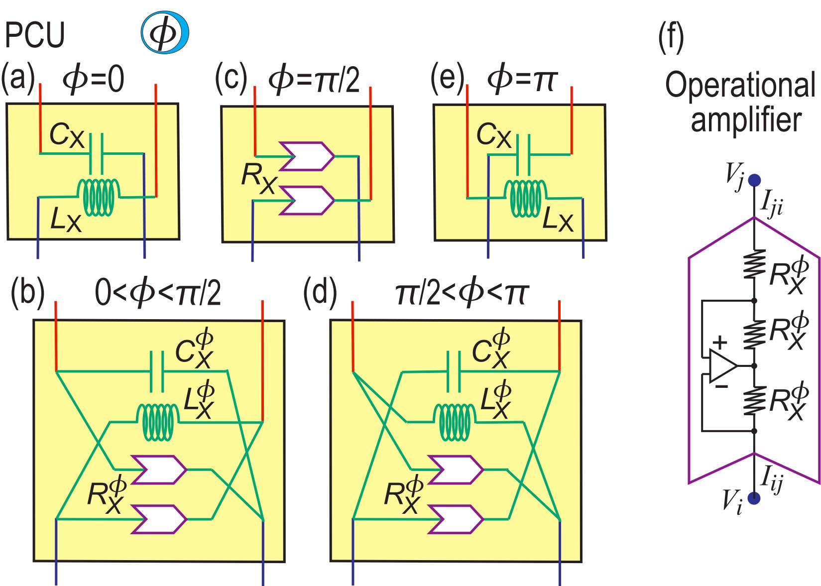
Figure 11: Illustrations of a PCU. (a)$\sim$(e) Structure of a PCU for various values of $\phi$. It consists of capacitance $C_{X}^{\phi}$, inductance $L_{X}^{\phi}$ and operational amplifiers $R_{X}^{\phi}$. Their values are given by Eq.(146) to produce the "superconducting" phase $\phi$. (f) Structure of operational amplifierHofmann .

VII.3 PCU (phase-control unit)

As we have stated, Fig.3(a) is for the Kitaev $H_{\text{K}}^{y}$ model (7) by setting $\phi=0$ in the Kitaev $H_{\text{K}}$ model (3). The phase choice $\phi=0$ is made by the setting of the pairing interactions between the two main channels shown in green in Fig.3(b). We have made this point explicit in Fig.3(c) and (e), which is equivalent to Fig.3(b), by introducing the symbol of PCU at $\phi=0$. It is composed of the capacitor $C_{X}$ and the inductor $L_{X}$.

It is necessary to include the phase degree of freedom associated with $\phi$ to make a braiding. We have considered the case with $\phi=\pi/2$ in a previous workEzawaMajo , where we have used operational amplifies $R_{X}$. An operational amplifier is illustrated in Fig.11(f), which acts as a negative impedance converter with current inversionHofmann . In the operational amplifier, the resistance depends on the current flowing direction; $R_{X}$ for the forward flow and $-R_{X}$ for the backward flow with the convention that $R_{X}>0$.

We illustrate PCU at $\phi=0$, $0<\phi<\pi/2$, $\pi/2$, $\pi/2<\phi<\pi$ and $\phi=\pi$ in Fig.11(a)$\sim$(e). We explain how the circuit Laplacian and the electric circuit are modified for each case. The structure of PCU is determined only by modifying the pairing interactions between the two main channels. Hence, the diagonal components $h_{1}$ and $h_{2}$ are not affected in the circuit Laplacian (131).

(i) At $\phi=\pi$, PCU is shown in Fig.11(a). The capacitors $C_{X}$ and the inductors $L_{X}$ are interchanged as compared with that at $\phi=0$. The circuit Laplacian is given by replacing Eqs.(133) with

$$g_{1} =(\omega_{0}^{2}L_{X})^{-1}e^{ik}-C_{X}e^{-ik},$$

$$g_{2} =-C_{X}e^{ik}+(\omega_{0}^{2}L_{X})^{-1}e^{-ik}.$$ (143)

(ii) At $\phi=\pi/2$, PCU is shown in Fig.11(c). The circuit is constructed with the use of operational amplifiers only, and the circuit Laplacian is given by

$$g_{1}=g_{2}=2(\omega_{0}R_{X})^{-1}\sin k.$$ (144)

(iii) For $0\leq\phi\leq\pi/2$, PCU is shown in Fig.11(b). It is necessary to use $C_{X}$, $L_{X}$ and $R_{X}$ as a function of $\phi$ to generate the Kitaev model with $\phi$. We study the case of the topological phase explicitly. The circuit Laplacian is given by replacing Eqs.(133) with

$$g_{1} =-C_{X}^{\phi}e^{ik}+(\omega_{0}^{2}L_{X}^{\phi})^{-1}e^{-ik}+2(\omega_{0}R_{X}^{\phi})^{-1}\sin k,$$

$$g_{2} =(\omega_{0}^{2}L_{X}^{\phi})^{-1}e^{ik}-C_{X}^{\phi}e^{-ik}+2(\omega_{0}R_{X}^{\phi})^{-1}\sin k.$$ (145)

By requiring Eqs.(134) and

$$C_{X}^{\phi}=C_{X}\left|\cos\phi\right|,\quad L_{X}^{\phi}=\frac{L_{X}}{\left|\cos\phi\right|},\quad R_{X}^{\phi}=\frac{R_{X}}{\left|\sin\phi\right|},$$ (146)

the circuit Laplacian is reduced to

$$J=\left[2C(1-\cos k)-C_{0}\right]\sigma_{z}+2\left(\frac{\sqrt{LC}}{R_{X}^{\phi}}\sigma_{x}+C_{X}^{\phi}\sigma_{y}\right)\sin k.$$ (147)

Formulas (146) are valid for arbitrary $\phi$. In particular, when we set $\phi\rightarrow 0$, all these equations are reduced to those in Sec.VII.2. On the other hand, when we set $\phi\rightarrow\pi/2$, Eqs.(145) are reduced to Eqs.(144). A similar analysis is made with respect to the trivial phase.

(iv) For $\pi/2\leq\phi\leq\pi$, PCU is shown in Fig.11(d). We study the topological phase explicitly. The circuit Laplacian is given by replacing Eqs.(133) with

$$g_{1} =(\omega_{0}^{2}L_{X}^{\phi})^{-1}e^{ik}-C_{X}^{\phi}e^{-ik}+2(\omega_{0}R_{X}^{\phi})^{-1}\sin k,$$

$$g_{2} =-C_{X}^{\phi}e^{ik}+(\omega_{0}^{2}L_{X}^{\phi})^{-1}e^{-ik}+2(\omega_{0}R_{X}^{\phi})^{-1}\sin k.$$ (148)

The circuit Laplacian is reduced to

$$J=\left[2C(1-\cos k)-C_{0}\right]\sigma_{z}+2\left(\frac{\sqrt{LC}}{R_{X}^{\phi}}\sigma_{x}-C_{X}^{\phi}\sigma_{y}\right)\sin k,$$ (149)

by requiring Eqs.(146). We note that, when we set $\phi\rightarrow\pi/2$, Eqs.(148) are reduced to Eqs.(144).

Consequently, when we use $C_{X}^{\phi}$, $L_{X}^{\phi}$ and $R_{X}^{\phi}$ defined by Eqs.(146) within PCU, the Kitaev model with arbitrary $\phi$ is realized in electric circuits.

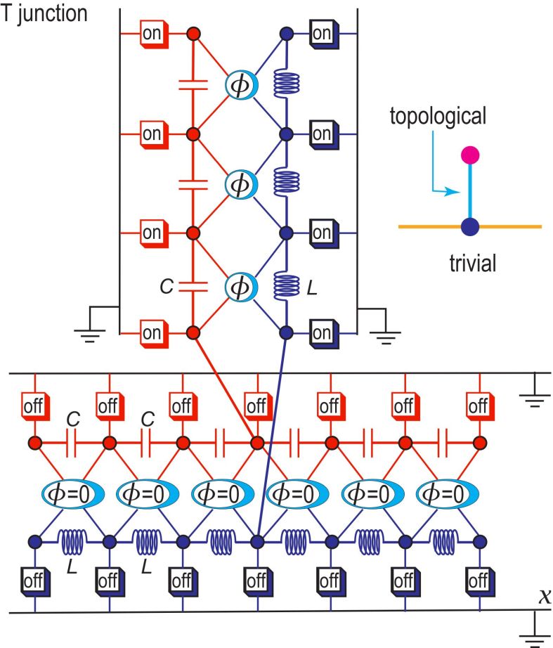
Figure 12: (a) Illustrations of an electric circuit for a T-junction in terms of TCUs and PCUs. The horizontal part is essentially the same as the one in Fig.3 except that it is entirely in the trivial phase. This circuit is for the configurations in Fig.7(d) and (e), where the horizontal leg-1 and leg-2 are trivial while the vertical leg-3 is topological.

VII.4 T-junction

A T-junction may be designed in electric circuits as in Fig.12. This circuit is for the configurations in Fig.7(d), where the horizontal leg-1 and leg-2 are trivial while the vertical leg-3 is topological. When all TCUs are set on, it is for the configurations in Fig.9(d), where all three legs are topological.

During a braiding process, it is necessary to control $\phi$ continuously from $\phi=0$ to $\phi=\pi$ to proceed from (d) to (e) in Fig.7 and Fig.9. A similar control is necessary from (h) to (i) in these figures. Such an operation is made possible by using a rotary switch tuning variable parameters $R^{\phi}$, $C_{X}^{\phi}$ and $L_{X}^{\phi}$ within a PCU according to the formula (146), as we discuss later.

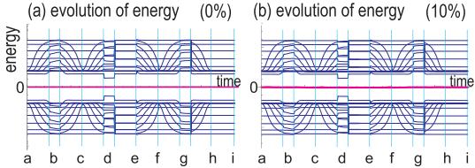
Figure 13: Evolution of the energy as a function of time, (a) without any randomness (0%), and (b) with 10% randomness on the on-site potential. Figure (a) is the same as Fig.8(b). The energy of the edge states (in red) are found to slightly deviate from zero by randomness in (b).

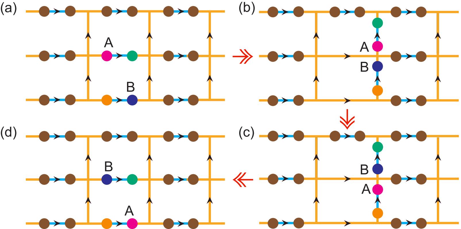
Figure 14: Non-Abelian braiding of Majorana states deposited on a square network. Topological segments (cyan) are created on horizontal parallel Kitaev chains, which are connected by vertical parallel Kitaev chains. A crossroads may be used as a T-junction for two edges to braid. In this example two edges A (in red) and B (in blue) on different parallel chains are braided by following the steps (a), (b), (c) and (d).

VIII Discussions

We have explored the physics associated with topological edge states in an electric circuit whose circuit Laplacian is equivalent to the Hamiltonian for the Kitaev $p$-wave superconductor. The circuit contains two main channels (capacitor channel and inductor channel) corresponding to the electron band and hole band. The position and the phase of an edge soliton are externally controlled by TCUs and PCUs, respectively, and observable by an impedance peak.

The braiding of edge states is performed with the aid of T-junction. In particular, we have derived the one-qubit (two-qubit) gate resulting from the braiding of two edge states across a topological (trivial) segment. The results agree precisely with those obtained based on Majorana fermions in superconducting systems. Consequently, quantum gates based on our electric circuits will be entirely equivalent to the standard quantum gates based on Majorana fermions. A merit of electric circuit realization is that we can exactly set the critical point $t=\Delta$, which is practically impossible in topological superconductors. Recall that the edge states are exactly localized when $t=\Delta$.

We have shown that quantum gates are constructed in electric circuits provided PHS is intact. In actual electric circuits, PHS will be broken weakly due to the randomness, which acts as the on-site potential randomness. We show the energy spectrum evolution in the presence of the 10% on-site potential randomness in Fig.13. Although the edge states acquire slight non-zero values, they are well separated from the bulk spectrum. They evolve smoothly as a function of time since the randomness is solely determined by sample elements which are fixed during time evolution. Furthermore, it is possible to make fine tuning of sample elements in the electric circuit for a practical degeneracy of edge states. We should mention that, once fine tuning is made, we can use it for good.

By generalizing a one-dimensional array of the T-junctions to the two dimensions, it becomes possible to braid edge states on a square lattice, which is illustrated in Fig.14. In the same way, we can generalize them to the three dimensions, where edge states are deposited on a cube.

Some ingenuity might be necessary in actual implementation of integrated circuits. Varactor (variable capacitance diode) will be useful to control the capacitanceGarcia . Inductors may be displaced by simulated inductorsSimL with the use of operational amplifiers.

We have pursued the parallel between the Kitaev superconductor model hosting Majorana fermions and the Kitaev electric-circuit chain governed by the Kirchhoff laws. As we have shown, it is possible to introduce Majorana operators in the electric circuit. However, this does not mean that it is possible to construct a whole quantum system. A quantum system has two main properties: (i) A linear algebra structure and (ii) the contraction of the wave function. The electric-circuit system has the property (i) but not the property (ii). Let us explain a bit more in details.

Electric circuits can simulate qubits, unitary transformation, superposition and entanglement, as we have shown. This is so because they require only a linear algebra structure, which exists also in the Kirchhoff laws. On the other hand, they cannot simulate the contraction of the wave function, because there is no probabilistic phenomena in electric circuits. Accordingly, we cannot simulate such quantum algorithms that use the contraction of the wave function. In addition, electric circuits cannot simulate quantum communications such as quantum teleportation by the same reason. However, it is not so serious as a topological quantum computer. Indeed, most quantum algorithms based on the braiding of Majorana fermions do not require the contraction of the wave function.

The author is thankful to E. Saito, Y. Mita and N. Nagaosa for helpful discussions on the subject. This work is supported by the Grants-in-Aid for Scientific Research from MEXT KAKENHI (Grants No. JP17K05490, No. JP15H05854 and No. JP18H03676). This work is also supported by CREST, JST (JPMJCR16F1 and JPMJCR1874).

References

- (1) G. Moore and N. Read, Nucl. Phys. B 360, 362 (1991).
- (2) S. Das Sarma, M. Freedman, and C. Nayak, Phys. Rev. Lett. 94, 166802 (2005).
- (3) A. Kitaev, Annals of Physics 321, 2 (2006).
- (4) C. Nayak, S. H. Simon, A. Stern, M. Freedman, and S. Das Sarma, Rev. Mod. Phys. 80, 1083 (2008).
- (5) A. Stern, Ann. Physics 323, 204 (2008).
- (6) A. Stern, Nature 464, 187 (2010).
- (7) S. Das Sarma, M. Freedman, C. Nayak, npj Quantum Information 1, 15001 (2015).
- (8) P. Bonderson, V. Gurarie and C. Nayak. Phys. Rev. B 83, 075303 (2011).
- (9) M. Cheng, V. Galitski and S. Das Sarma. Phys. Rev. B 84, 104529 (2011).
- (10) T. E. Pahomi, M. Sigrist, A. A. Soluyanov, arXiv:1904.07822.
- (11) J. Alicea, Y. Oreg, G. Refael, F. von Oppen and M.P.A. Fisher, Nat. Phys. 7, 412 (2011).
- (12) X.-L. Qi, S.-C. Zhang, Rev. Mod. Phys. 83, 1057 (2011).
- (13) J. Alicea, Rep. Prog. Phys. 75, 076501 (2012).
- (14) M. Leijnse and K. Flensberg, Semicond. Sci. Technol. 27, 124003 (2012).
- (15) C. W.J. Beenakker, Annu. Rev. Condens. Matter Phys. 4, 113 (2013).
- (16) T. D. Stanescu and S. Tewari, J. Phys. Condens. Matter 25, 233201 (2013).
- (17) S.R. Elliott and M. Franz, Rev. Mod. Phys. 87, 137 (2015).
- (18) M. Sato and Y. Ando, Rep. Prog. Phys. 80, 076501 (2017).
- (19) C. W. J. Beenakker, SciPost Phys. Lect. Notes 15 (2020)
- (20) D. Aasen, M. Hell, R. V. Mishmash, A. Higginbotham, J. Danon, M. Leijnse, T. S. Jespersen, J. A. Folk, C. M. Marcus, K. Flensberg, and J. Alicea, Phys. Rev. X 6, 031016 (2016).
- (21) C. V. Kraus, P. Zoller and M. A. Baranov, Phys. Rev. Lett. 111, 203001 (2013).
- (22) D. A. Ivanov Phys. Rev. Lett. 86, 268, (2001).
- (23) B. I. Halperin, Y. Oreg, A. Stern, G. Refael, J. Alicea and F. von Oppen, Phys. Rev. B 85, 144501 (2012).
- (24) K. Snizhko, R. Egger and Y. Gefen, Phys. Rev. Lett. 123, 060405 (2019).
- (25) M. Z. Hasan and C. L. Kane, Rev. Mod. Phys. 82, 3045 (2010).
- (26) Z. Yang, F. Gao, X. Shi, X. Lin, Z. Gao, Y. Chong and B. Zhang, Phys. Rev. Lett. 114, 114301 (2015).
- (27) P. Wang, L. Lu and K. Bertoldi, Phys. Rev. Lett. 115, 104302 (2015).
- (28) R. Ssstrunk and S. D. Huber, Proc. Natl. Acad. Sci. USA 113, E4767 (2016).
- (29) C. He, X. Ni, H. Ge, X.-C. Sun,Y.-B. Chen1 M.-H. Lu, X.-P. Liu, L. Feng and Y.-F. Chen, Nature Physics 12, 1124 (2016).
- (30) A. B. Khanikaev, S. H. Mousavi, W.-K. Tse, M. Kargarian, A. H. MacDonald, G. Shvets, Nature Materials 12, 233 (2013).
- (31) M. Hafezi, E. Demler, M. Lukin, J. Taylor, Nature Physics 7, 907 (2011).
- (32) M. Hafezi, S. Mittal, J. Fan, A. Migdall, J. Taylor, Nature Photonics 7, 1001 (2013).
- (33) L.H. Wu and X. Hu, Phys. Rev. Lett. 114, 223901 (2015).
- (34) L. Lu. J. D. Joannopoulos and M. Soljacic, Nature Photonics 8, 821 (2014).
- (35) T. Ozawa, H. M. Price, A. Amo, N. Goldman, M. Hafezi, L. Lu, M. C. Rechtsman, D. Schuster, J. Simon, O. Zilberberg and L. Carusotto, Rev. Mod. Phys. 91, 015006 (2019).
- (36) L. M. Nash, D. Kleckner, A. Read, V. Vitelli, A. M. Turner and W. T. M. Irvine, PNAS, 112, 14495 (2015).
- (37) S. D. Huber, Nature Physics 12, 621 (2016).
- (38) S. Imhof, C. Berger, F. Bayer, J. Brehm, L. Molenkamp, T. Kiessling, F. Schindler, C. H. Lee, M. Greiter, T. Neupert, R. Thomale, Nat. Phys. 14, 925 (2018).
- (39) C. H. Lee , S. Imhof, C. Berger, F. Bayer, J. Brehm, L. W. Molenkamp, T. Kiessling and R. Thomale, Communications Physics, 1, 39 (2018).
- (40) M. Ezawa, Phys. Rev. B 100, 045407 (2019).
- (41) N. Read and D. Green, Phys. Rev. B 61, 10267 (2000).
- (42) A. Kitaev, Phys. Usp. 44 (suppl.), 131 (2001).
- (43) T. Helbig, T. Hofmann, C. H. Lee, R. Thomale, S. Imhof, L. W. Molenkamp and T. Kiessling, Phys. Rev. B 99, 161114 (2019).
- (44) Y. Lu, N. Jia, L. Su, C. Owens, G. Juzeliunas, D. I. Schuster and J. Simon, Phys. Rev. B 99, 020302 (2019).
- (45) K. Luo, R. Yu and H. Weng, Research (2018), ID 6793752.
- (46) E. Zhao, Ann. Phys. 399, 289 (2018).
- (47) M. Ezawa, Phys. Rev. B 98, 201402(R) (2018).
- (48) M. Serra-Garcia, R. Susstrunk and S. D. Huber, Phys. Rev. B 99, 020304 (2019).
- (49) T. Hofmann, T. Helbig, C. H. Lee, M. Greiter, R. Thomale, Phys. Rev. Lett. 122, 247702 (2019).
- (50) M. Ezawa, Phys. Rev. B 99, 201411(R) (2019).
- (51) R. Haenel, T. Branch, M. Franz, Phys. Rev. B 99, 235110 (2019).
- (52) M. Ezawa, Phys. Rev. B 99, 121411(R) (2019).
- (53) X. X. Zhang and M. Franz, Phys. Rev. Lett. 124, 046401 (2020).
- (54) F. Wilczek and A. Zee, Phys. Rev. Lett. 52, 2111 (1984).
- (55) J. K. Pachos, Introductioni to topological quantum computation, Cambridge University Press, Cambridge (2012).
- (56) T. D. Stanescu, Introduction to topological quantum matter and quantum computation, CRC press, Boca Raton, Florida (2016).
- (57) D. Aasen, M. Hell, R. V. Mishmash, A. Higginbotham, J. Danon, M. Leijnse, T. S. Jespersen, J. A. Folk, C. M. Marcus, K. Flensberg, and J. Alicea, Phys. Rev. X, 6, 031016 (2016).
- (58) S. Coleman, Phys. Rev. D 11, 2088 (1975).
- (59) S. Mandelstam, Phys. Rev. D 11, 3026 (1975).
- (60) W. Thirring, Ann. Phys. 3, 91 (1958).
- (61) D.F. Berndt and S. C. Dutta Roy, IEEE Journal of Solid-State Circuits, SC-4: 161 (1969).