Abstract

In this paper the planar orbit and attitude dynamics of an uncontrolled spacecraft is studied, taking on-board a deorbiting device. Solar and drag sails with the same shape are considered and separately studied. In both cases, these devices are assumed to have a simplified pyramidal shape that endows the spacecraft with helio and drag stable properties. The translational dynamics is assumed to be planar and hence the rotational dynamics occurs only around one of the principal axes of the spacecraft. Stable or slowly-varying attitudes are studied, subject to disturbances due to the Earth oblateness effect and gravity gradient torques, and either solar radiation pressure or atmospheric drag torque and acceleration. The results are analysed with respect to the aperture of the sail and the center of mass - center of pressure offset.

Nomenclature

$\alpha$  =	aperture angle of the sail, deg or rad
$d$  =	center of mass - center of pressure offset, m
$h$  =	height of the panels, m
$w$  =	width of the panels, m
$A_{s}$  =	area of the panels, m2
$m_{s}/2$  =	mass of the panels, kg
$m_{b}$  =	mass of the bus, kg
$\mathcal{F}_{b}$  =	body frame
$\xi,\eta,\zeta$  =	coordinates of $\mathcal{F}_{b}$
${\bf i}_{\xi},{\bf i}_{\eta},{\bf i}_{\zeta}$  =	unit vectors of the basis of $\mathcal{F}_{b}$
$A,B,C$  =	inertia moments of the whole spacecraft, kg m2
$P$  =	panels / parametrization of the panels in $\mathcal{F}_{b}$
${\bf n}$  =	normal vectors to panels
$\mathcal{F}_{I}$  =	Earth centered inertial frame
$x,y,z$  =	coordinates of $\mathcal{F}_{I}$
${\bf i}_{x},{\bf i}_{y},{\bf i}_{z}$  =	unit vectors of the basis of $\mathcal{F}_{I}$
$\phi,\Phi$  =	Euler angle and angular velocity of the attitude, rad or deg, /s
$\lambda$  =	Angle between Sun position and ${\bf i}_{x}$, rad or deg
$p_{\rm SR}$  =	solar radiation pressure at 1 AU, N/m2
$\delta$  =	flight path angle, rad or deg
$\rho$  =	atmospheric density, kg/m3
$C_{D}$  =	drag coefficient
${\bf u}$  =	unit vector
${\bf r},r$  =	position vector and its magnitude, km
${\bf v},r$  =	velocity vector and its magnitude, km/s
${\bf M},M$  =	torque vector, component of torque vector, N m
${\bf F}$  =	force vector, N
$\sigma_{1,2,3}$  =	cosines of the Earth-Sun vector in $\mathcal{F}_{b}$
$\gamma_{1,2,3}$  =	cosines of the Earth-spacecraft vector in $\mathcal{F}_{b}$
$\nu_{1,2,3}$  =	cosines of the relative velocity vector in $\mathcal{F}_{b}$
$\Sigma$  =	Surface of section where Poincaré iterates are computed
$a$  =	semi-major axis of the spacecraft’s orbit
$e$  =	eccentricity of the spacecraft’s orbit
$\Omega$  =	Right ascension of the ascending node of the spacecraft’s orbit
$\omega$  =	argument of the perigee of the spacecraft’s orbit, measured from ascending node

Subscripts and upperscripts

$\pm$  =	that refers to panels $+$ or $-$
$S$  =	that refers to Earth-Sun
${\rm sc}$  =	that refers to spacecraft-Earth
${\rm rel}$  =	that refers to the relative velocity with respect to the atmosphere
$\xi,\eta,\zeta$  =	in the direction of, in $\mathcal{F}_{b}$
$x,y,z$  =	in the direction of, in $\mathcal{F}_{I}$

1 Introduction

Solar sails are a low-thrust propulsion that relies on the Solar Radiation Pressure (SRP). They have attracted much attention in the literature, since a spacecraft with a solar sail generated acceleration in a slow but continuous way allowing to reduce the cost of missions. This technology has been successfully demonstrated in various missions, see for instance JAXA’s IKAROS [18], the Planetary Society’s LightSail projects and NASA’s NanoSail-D project [10]. The latter demonstrated the feasibility of the deployment of a sail and its usage to deorbit a spacecraft exploiting the effect of atmospheric drag.

There is a vast literature on how to use the enhancements of the effects of SRP and drag for mission design. A common feature among these works is to assume that, along the trajectories, the attitude of the sail is fixed; hence the feasibility of these works rely on attitude control.

In this work and we build on studies whose objectives are end-of-life disposals employing sails as passive deorbiting devices. For deorbiting from an altitude where atmospheric drag is the dominant effect, the sail can be either controlled, to keep always its maximum cross area perpendicular to the incoming air flow, or uncontrolled and therefore tumbling. In this case the cross area exposed to aerodynamic drag will be varying in time [5]. For orbit altitude above 800 km, the effect of SRP can be exploited to achieve deorbiting. Deorbiting strategies making use of SRP can be splitted in two main attitude control strategies, active and passive, as defined in [3]. Active strategies allow deorbiting “inwards” on a spiraling path by decreasing the semi-major axis of the orbit. This is achieved by maximizing the SRP effect when approaching the Sun and minimizing it when moving away from the Sun [1], see the left panel in Figure 1. On the other hand, the passive approach requires a fixed attitude of the spacecraft with respect to the Sun, and it consists of the counter-intuitive idea of deorbiting “outwards” by increasing the eccentricity of the orbit, since this implies the decrease of the perigee [13, 14], see the right panel in Figure 1.

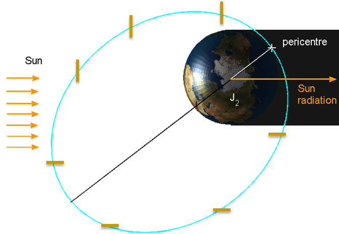
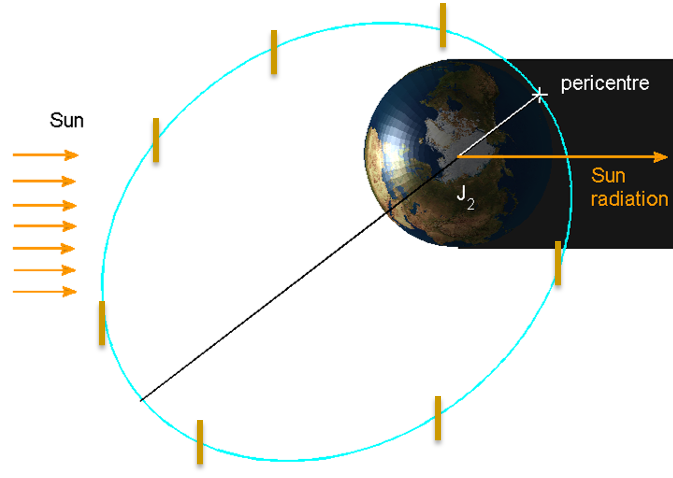
Figure 1: Sail orientation in the active (left) and the passive (right) deorbiting strategies [3].

Here the following natural question arises: can one find a sail with auto-stabilizing properties, so that the already cited strategies can apply minimizing the need for attitude control? The answer is affirmative from the point of view of SRP, and it is achieved by means of a Quasi-Rhombic Pyramid (QRP) shape, as suggested in [2]. The structure is formed by 4 reflective panels resembling the shape of the pyramid. If oriented towards the sunlight, such a structure is expected to compensate, on average, the components of the acceleration in any other direction. Namely, in [7] the authors provide a first-order (and hence local) argument for the stability of the sun-pointing attitude, and they later study the possible stability enhancements of assuming a moderate spin around this direction in [8].

Despite the authors of [2, 7, 8] obtain satisfactory results by considering such structure, there is, to the author’s knowledge, a lack of understanding on the stability from a more global point of view. That is, if there are also stable attitude dynamics close to the sun-pointing orientation, and, in affirmative case, if one can measure and describe the set of stable motion. This paper is a first step in this direction.

The goal of this paper is to give evidence of the possibilities of QRP as feasible auto-stabilized deorbiting devices both in SRP dominated regions and in atmospheric drag dominated regions, that are studied separately. The motion is assumed to be planar -the obliquity of the ecliptic is set to zero and the rotations occur around an axis perpendicular to the orbital plane- and the QRP is simplified so that out-of-plane motion is avoided. Also, the effect of eclipses is neglected. The attitude stability study takes into account two main parameters: aperture angle of the sail structure, $\alpha$ and the center of Mass - center of Pressure Offset (MPO), that is a signed real variable $d$.

The paper is structured as follows. First of all § 2 is devoted to the study of the geometry of the spacecraft under consideration and to provide their inertia moments taking into account the parameters $\alpha$ and $d$. This is used in § 3 to provide explicit expressions for the SRP, atmospheric drag and gravity gradient torques. This allows to set the equations of motion to be studied.

The next two sections are devoted to investigate attitude stability of the family of spacecraft under consideration in SRP dominated regions and in atmospheric drag dominated regions.

1. On the one hand, the hypotheses considered allow to start § 4 by approximating the dynamics as a one and a half degrees of freedom Hamiltonian system that allows to study separately SRP and gravity gradient torques as main effect and perturbation, respectively. This allows, in particular, to establish necessary physical relations between $\alpha$ and $d$ for helio-stability. The model is validated comparing the results with the integration of the full coupled orbit and attitude model in two test cases.

2. The analogous problem taking into account drag instead of SRP is considered in § 5. The differences and common features between both scenarios are first compared and a numerical study of the performance of the spacecraft under consideration as orbiting devices is performed.

This contribution ends in § 6 with a summary of the obtained results, conclusions and future lines of research that emerge from this paper.

2 Geometry of the sail

To avoid out-of-plane motion one is lead to consider a simplification of a QRP that consists of two panels of equal size; say of height $h$, width $w$, and area $A_{s}=hw$. Assume that the weight of each panel is $m_{s}/2$, so the mass of the whole sail structure is $m_{s}$. In the left panel of Fig. 2 a sketch of the sail structure is depicted. The right panel is a top view of the left sketch.

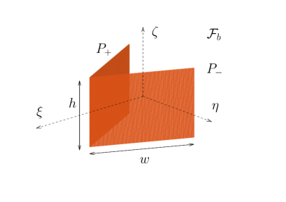
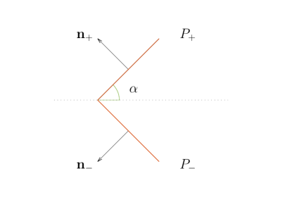
Figure 2: Sketch of the sail structure. Left: 3D view. Right: top view.

The parametrisation of the sail panels is written in a reference frame $\mathcal{F}_{b}$ attached to the spacecraft whose coordinates are $\xi,\eta$ and $\zeta$. Call ${\bf i}_{\xi,\eta,\zeta}$ the vectors of the basis. In the cylindrical coordinates $(r,\alpha,\zeta)$, $r=\xi^{2}+\eta^{2}$ and $\tan\alpha=\eta/\xi$, the panels of the sail are considered to be parametrized as

$$P_{+}\cup P_{-}, P_{\pm}=\left\{\left({\tt aux}-r\cos\alpha,\pm r\sin\alpha,\zeta\right)^{\top}:\;r\in[0,w],\;\zeta\in[-h/2,h/2]\right\},$$ (1)

where ${\tt aux}$ is a free parameter that will be chosen so that the center of mass of the whole spacecraft is at the origin of $\mathcal{F}_{b}$. The panels are attached to each other along an $h$-long side, that lies on a line parallel to the $\zeta$ axis, and they form an angle $\alpha$ with respect to the plane $\eta=0$. Assuming uniform density of the panels, the centre of mass of the structure is at

$${\bf r}_{s}=\left({\tt aux}-\frac{1}{2}w\cos\alpha,0,0\right)^{\top}.$$

Note that chosen this way, the principal axes of inertia of the sail are parallel to those of $\mathcal{F}_{b}$, and this remains true if the center of mass of the bus of the satellite lies on the $\xi$ axis. So, assume that the latter is located at the point ${\bf r}_{s}+(d,0,0)^{\top}$, $d\in\mathbb{R}$. The parameter $d$ accounts for the MPO, and its sign informs about the relative position of the payload with respect to the sail. The centre of mass of the whole spacecraft is the origin if

$${\tt aux} = \frac{1}{2}w\cos\alpha-d\frac{m_{b}}{m_{b}+m_{s}},$$ (2)

where $m_{b}$ is the mass of the bus of the spacecraft. Sketches of top views of spacecraft in $\mathcal{F}_{b}$ can be seen in Fig. 3, where the bus is depicted as a solid black dot. The left, center and right panels are sketches of spacecraft with $d<0$, $d=0$ and $d>0$, respectively. Note that, in particular, the bus is placed at the tip of the sail (where both panels are in contact) if we choose $d$ such that ${\tt aux}=0$ in Eq. 2, that is,

$$d = \frac{1}{2}w\cos(\alpha)\frac{m_{b}+m_{s}}{m_{b}}.$$ (3)

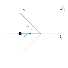
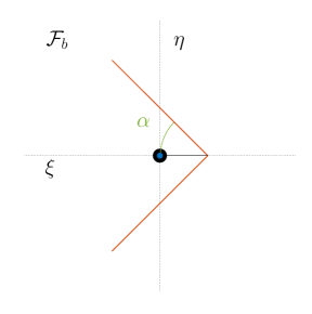
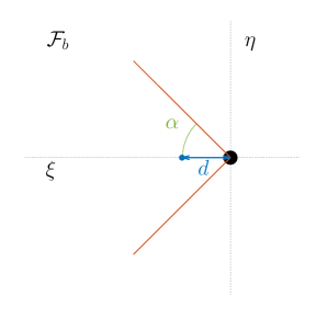
Figure 3: Sketch of the top view of the spacecraft in $\mathcal{F}_{b}$, where the bus is depicted as a solid circle. Left: $d<0$. Center: $d=0$. Right: $d>0$.

Assume that the principal axes of the payload are also parallel to the axes of $\mathcal{F}_{b}$, and denote $I_{\xi,b},I_{\eta,b}$ and $I_{\zeta,b}$ its moments of inertia if its centre of mass is at the origin. Using the parallel axes theorem see, e.g. [9], the moments of inertia along the $\xi$, $\eta$ and $\zeta$ axes of the whole spacecraft are, respectively,

$$A=I_{\xi,b}+\frac{h^{2}m_{s}}{6},\quad B=I_{\eta,b}+\frac{h^{2}m_{s}}{6}+D(\alpha,d),\quad C=I_{\zeta,b}+D(\alpha,d),$$ (4a)

$$D(\alpha,d)=\frac{1}{6}m_{s}w^{2}\cos^{2}\alpha+\frac{d^{2}m_{b}^{2}(m_{b}+2m_{s})}{(m_{b}+m_{s})^{2}}$$ (4b)

Finally, denote ${\bf n}_{\pm}=(\sin\alpha,\pm\cos\alpha,0)$ the normal vector of the panels $P_{\pm}$, see the right sketch in Fig. 2.

3 Model of planar orbit and attitude dynamics

The planar orbit and attitude dynamics considered here is a coupled system of differential equations in $(\mathbb{S}^{1}\times\mathbb{R})\times\mathbb{R}^{4}$, where $\mathbb{S}^{1}:=\mathbb{R}/(2\pi\mathbb{Z})$: orientation and angular velocity of the rotational dynamics in $\mathcal{F}_{b}$ and position and velocity of the spacecraft in an Earth centered inertial frame $\mathcal{F}_{I}$. Denote the coordinates of $\mathcal{F}_{I}$ $x,y$ and $z$, and the vectors of the orthonormal basis ${\bf i}_{x,y,z}$. The vector ${\bf i}_{x}$ points towards an arbitrarily chosen direction on the ecliptic (e.g. J2000), and since the dynamics in this paper is restricted to the plane, the vectors ${\bf i}_{z}$ and ${\bf i}_{\zeta}$ are parallel. The triad is completed by choosing ${\bf i}_{y}={\bf i}_{z}\times{\bf i}_{x}$.

This section deals with vectors in the two frames $\mathcal{F}_{I}$ and $\mathcal{F}_{b}$. To avoid confusion and unless a formula that applies in both frames is given, the subscript $I$ and $b$ refer to vectors in $\mathcal{F}_{I}$ and $\mathcal{F}_{b}$, respectively.

In the case planar motion, the rotation dynamics of the spacecraft is fully explained using a single Euler angle, $\varphi\in[0,2\pi)$. Assume the change of coordinates from $\mathcal{F}_{I}$ to $\mathcal{F}_{b}$ is done through $R_{3}(-\varphi)$, where

$$R_{3}(\psi)=\left(\begin{array}[]{rrc}\cos\psi&-\sin\psi&0\\ \sin\psi&\cos\psi&0\\ 0&0&1\end{array}\right).$$

The Euler equations in this situation reduce to

$$C\ddot{\varphi} = M_{\zeta}\qquad\mbox{ or }\qquad\left\{\begin{array}[]{rcl}\dot{\varphi}&=&\Phi\\ \dot{\Phi}&=&M_{\zeta}/C\end{array}\right.,$$ (7)

where $\Phi$ is the rotational angular velocity and $C$ is the third inertia moment, recall Eq. 4a, and $M_{\zeta}$ refers to the sum of the components along the $\zeta$ direction of the torques under consideration, that will be derived in § 3.1. The state vector of the complete problem is of the form

$$\left[\varphi,\;\Phi,\;x,\;y,\;v_{x},\;v_{y}\right]^{\top}.$$

3.1 Orbit and attitude perturbations

Assume that the apparent motion of the Sun around the Earth is circular with constant angular velocity $n_{\odot}$, and let $\lambda$ denote the angle of position of the Sun on the orbital plane with respect to ${\bf i}_{x}$. In the frames $\mathcal{F}_{I}$ and $\mathcal{F}_{b}$ the Earth-Sun vector reads

$${\bf u}_{S,I} = (\cos\lambda,\sin\lambda,0)^{\top}_{I},\quad{\bf r}_{S,I}=r_{S}{\bf u}_{S,I};\quad{\bf u}_{S,b}=R_{3}(-\varphi){\bf u}_{S,I},\quad{\bf r}_{S,b}=r_{S}{\bf u}_{S,b}.$$ (8)

On the other hand, the Earth-spacecraft vector in the $\mathcal{F}_{I}$ and $\mathcal{F}_{b}$ frames read

$${\bf u}_{{\rm sc},I} = (\cos\vartheta,\sin\vartheta,0)^{\top}_{I},\quad{\bf r}_{{\rm sc},I}=r_{\rm sc}{\bf u}_{{\rm sc},I};\quad{\bf u}_{{\rm sc},b}=R_{3}(-\varphi){\bf u}_{{\rm sc},I},\quad{\bf r}_{{\rm sc},b}=r_{\rm sc}{\bf u}_{{\rm sc},b},$$ (9)

where $r_{\rm sc}=\sqrt{x^{2}+y^{2}}$ and $\vartheta=\Omega+\omega+\theta$, being $\Omega$ the Right Ascension of the Ascending Node (RAAN), $\omega$ is the argument of the perigee and $\theta$ is the true anomaly of the osculating orbit.

Finally the relative velocity of the spacecraft with respect to the atmosphere reads, in the $\mathcal{F}_{I}$ and $\mathcal{F}_{b}$ frames

$${\bf u}_{{\rm rel},I}=(\cos\delta,\sin\delta,0)^{\top}_{I},\quad{\bf v}_{{\rm rel},I}=v_{\rm rel}{\bf u}_{{\rm rel},I};\quad{\bf u}_{{\rm rel},b}=R_{3}(-\varphi){\bf u}_{{\rm rel},I},\quad{\bf v}_{{\rm rel},b}=v_{\rm rel}{\bf u}_{{\rm rel},b},$$ (10)

where $\delta:=\arctan(v_{y}/v_{x})$ and $v_{\rm rel}=\sqrt{v_{x}^{2}+v_{y}^{2}}$. In Fig. 4 a sketch of the considered motion and the vectors ${\bf r}_{S},{\bf r}_{\rm sc}$ and ${\bf v}_{\rm rel}$ is shown.

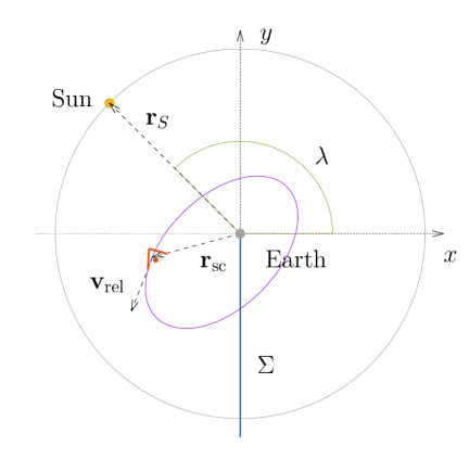
Figure 4: Sketch of the main elements that play a role in the dynamics of the studied family of spacecraft.

For convenience, let us denote

$${\bf u}_{S,b} := \sigma_{1}{\bf i}_{\xi}+\sigma_{2}{\bf i}_{\eta}+\sigma_{3}{\bf i}_{\zeta},$$ (11a)

$${\bf u}_{{\rm sc},b} := \gamma_{1}{\bf i}_{\xi}+\gamma_{2}{\bf i}_{\eta}+\gamma_{3}{\bf i}_{\zeta},$$ (11b)

$${\bf u}_{{\rm rel},b} := \nu_{1}{\bf i}_{\xi}+\nu_{2}{\bf i}_{\eta}+\nu_{3}{\bf i}_{\zeta},$$ (11c)

where

$$\sigma_{1}^{2}+\sigma_{2}^{2}+\sigma_{3}^{2}\;=\;\gamma_{1}^{2}+\gamma_{2}^{2}+\gamma_{3}^{2}\;=\;\nu_{1}^{2}+\nu_{2}^{2}+\nu_{3}^{2}\;=\;1$$

are direction cosines.

The shape of the sail structure in Fig. 2 makes the torques due to SRP and drag acceleration have a different representation depending on how the sail is oriented with respect to the sunlight or relative velocity vectors, respectively. Since the scope of this paper are stable motions close to either the sun-pointing or velocity-pointing directions, we are only lead to consider the following cases:

1. For SRP, denote $\phi=\varphi-\lambda$. If $\phi\in(-\alpha,\pi-\alpha)$, the panel $P_{-}$ produces acceleration and torque; and if $\phi\in(-\pi+\alpha,\alpha)$, the panel $P_{+}$ does; in particular, if $|\phi|<\alpha$, both panels face the sunlight.

2. For atmospheric drag, let $\hat{\phi}=\varphi-\delta$. Similarly, if $\hat{\phi}\in(-\alpha,\pi-\alpha)$, the panel $P_{-}$ produces acceleration and torque, if $\hat{\phi}\in(-\pi+\alpha,\alpha)$, the panel $P_{+}$ does, and for $|\hat{\phi}|<\alpha$ both do.

This is sketched in Fig. 5, where the three cases are exemplified: in the sketch $\lambda=180^{\circ}$ and if so, both $P_{\pm}$ produce torque in (1), and only $P_{+}$ in (3) and only $P_{-}$ in (2).

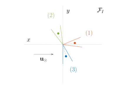
Figure 5: Sketch of different orientations of the Sail in the $\mathcal{F}_{I}$ frame in the case of SRP, where $\lambda$ is depicted as being $180^{\circ}$. If oriented as depicted, only $P_{+}$ (resp. $P_{-}$) produces torque for (2) (resp. (3)), while both panels do in (1).

3.1.1 Solar radiation pressure

The force due to SRP exerted in each panel of the sail is assumed to be partially specularly reflected and partially absorbed [15]

$${\bf F}_{\rm SRP}^{\pm} = -p_{\rm SR}A_{s}({\bf n}_{\pm}\cdot{\bf u}_{\rm S})\left(2\eta({\bf n}_{\pm}\cdot{\bf u}_{\rm S}){\bf n}_{\pm}+(1-\eta){\bf u}_{\rm S}\right),$$ (12)

where $\eta\in(0,1)$ is the (dimensionless) reflectance of the sail and $p_{\rm SR}=4.56\times 10^{-6}\;{\rm N}/{\rm m}^{2}$ is the solar pressure at 1 AU, that is considered to be constant.

On the one hand, transporting the normal vectors of the panels to $\mathcal{F}_{I}$, $R_{3}(\varphi){\bf n}_{\pm}$, one can see that the SRP acceleration due to the panel $P_{\pm}$ reads $(a_{x}^{\pm},a_{y}^{\pm},0)_{I}^{\top}$, where

$$a_{x}^{\pm} = \frac{A_{s}p_{\rm SR}}{m_{b}+m_{s}}\sin(\alpha\pm\lambda\mp\varphi)(\eta\cos(2\alpha\pm\lambda\mp 2\varphi)-\cos\lambda))$$ (13a)

$$a_{y}^{\pm} = \frac{A_{s}p_{\rm SR}}{m_{b}+m_{s}}\sin(\alpha\pm\lambda\mp\varphi)(\mp\eta\sin(2\alpha\pm\lambda\mp 2\varphi)-\sin\lambda)).$$ (13b)

Hence the acceleration due SRP can be written as

$$\frac{A_{s}p_{\rm SR}}{m_{b}+m_{s}}(a_{x},a_{y},0)_{I}^{\top},$$ (14)

where

$$(a_{x},a_{y},0)_{I}^{\top} \!\!=\!\! \frac{m_{b}+m_{s}}{A_{s}p_{\rm SR}}\left[(a_{x}^{+},a_{y}^{+},0)_{I}^{\top}\chi_{(-\alpha,\pi-\alpha)}(\varphi-\lambda)+(a_{x}^{-},a_{y}^{-},0)_{I}^{\top}\chi_{(-\pi+ \alpha,\alpha)}(\varphi-\lambda)\right].$$

Here

$$\chi_{I}:\mathbb{R}\to\{0,1\},\qquad\chi_{I}(\psi)=\left\{\begin{array}[]{rcl}1&\mbox{if}&\psi\in I\\ 0&\mbox{if}&\psi\notin I\\ \end{array}\right.$$

denotes the characteristic function of the interval $I$. This notation

Note that $a_{x}$ and $a_{y}$ just consist of the adimensional factors in Eq. 13. In the particular case that $\alpha=\pi/2$ and $\varphi=\lambda$, that is, when the sail is a rectangular flat panel with sides $2w$ and $w$, and the direction of the normal is parallel to the sun-spacecraft direction, then Eq. 14 reads

$$-2\frac{A_{s}p_{\rm SR}}{m_{b}+m_{s}}(1+\eta)(\cos\lambda,\sin\lambda,0)_{I}^{\top},$$

twice the acceleration of a flat square panel of size $w$ always oriented towards the Sun, see [3].

On the other hand, the torque due to SRP is ${\bf M}_{\rm SRP}={\bf M}_{\rm SRP}^{-}+{\bf M}_{\rm SRP}^{+},$ where ${\bf M}_{\rm SRP}^{\pm}={\bf r}_{\pm}\times{\bf F}_{\rm SRP}^{\pm}$, and ${\bf r}_{\pm}$ is the location of the center of mass of the sail panel $P_{\pm}$. Their third component $M_{\rm SRP,\zeta}^{\pm}$ reads

$$M_{\rm SRP,\zeta}^{\pm} = \frac{A_{s}}{m_{b}+m_{s}}\frac{p_{\rm SR}}{2}\left(k_{1,1}(\eta)\sigma_{1}\sigma_{2}\pm k_{2,0}(\eta)\sigma_{1}^{2}\pm k_{0,2}(\eta)\sigma_{2}^{2}\right),$$ (15)

where

$$k_{1,1}(\eta) = \sin\alpha\left[2dm_{b}(2\eta\cos(2\alpha)+\eta+1)+w(m_{b}+m_{s})(\cos\alpha-\eta\cos(3\alpha))\right],$$ (16a)

$$k_{2,0}(\eta) = \sin^{2}\alpha\left[4d\eta m_{b}\cos\alpha+w(m_{b}+m_{s})(1-\eta\cos(2\alpha))\right],\mbox{ and}$$ (16b)

$$k_{0,2}(\eta) = \cos\alpha\left[2dm_{b}(\eta\cos(2\alpha)+1)+\eta w(m_{b}+m_{s})\sin\alpha\sin(2\alpha)\right].$$ (16c)

Hence, using Eqs. 11 and 8 and assuming that $k_{1,1}(\eta)\neq 0$, the torque due to SRP can be written as follows: denoting

$$M_{0}^{\pm}(\psi,\eta)=-\frac{1}{2}\sin(2\psi)\pm\frac{k_{2,0}(\eta)}{k_{1,1}(\eta)}\cos^{2}\psi\pm\frac{k_{0,2}(\eta)}{k_{1,1}(\eta)}\sin^{2}\psi,$$ (17)

then

$$M_{\rm SRP} = \frac{A_{s}}{m_{b}+m_{s}}\frac{p_{\rm SR}k_{1,1}(\eta)}{2}M_{1}(\varphi-\lambda,\eta),\quad\mbox{ where}$$ (18a)

$$M_{1}(\psi,\eta) \!\!=\!\! M_{0}^{-}(\psi,\eta)\chi_{[-\alpha,\pi-\alpha]}(\psi)+M_{0}^{+}(\psi,\eta)\chi_{[-\pi+\alpha,\alpha]}(\psi)$$ (18b)

The functions $M_{0}^{\pm}$ has to be understood as the scaled torque due to $P_{\pm}$, and $M_{1}$ as the torque due to both panels at the same time, as it takes into account the orientation of the sunlight direction with respect to the panels.

The coefficients $k_{1,1},k_{2,0}$ and $k_{0,2}$ also depend on the masses $m_{b},m_{s}$, the parameters $\alpha,d$ and the width $w$, but only the dependence on $\eta$ is stressed for reasons that are clarified in § 3.1.2, that is devoted to the equations of the effects due to atmospheric drag.

3.1.2 Atmospheric drag

As for SRP the force due to atmospheric drag can be decomposed as the sum of the forces exerted to each of the two panels when experiencing air resistance. Due to the similarity with the procedure for SRP in § 3.1.1, some details of the derivation of the formulas are omitted.

The force due to drag of each panel can be written as [15]

$${\bf F}_{\rm drag}^{\pm} = -\frac{1}{2}\rho v_{\rm rel}^{2}C_{D}A_{s}({\bf n}_{\pm}\cdot{\bf u}_{\rm rel}){\bf u}_{\rm rel},$$ (19)

where $\rho$ is the atmospheric density and $C_{D}\in(1.5,2.5)$ is an empirically determined dimensionless drag coefficient.

On the one hand, the atmospheric drag acceleration due to $P_{\pm}$ reads $(b_{x}^{\pm},b_{y}^{\pm},0)_{I}^{\top}$, where

$$b_{x}^{\pm} = \frac{A_{s}\rho C_{D}}{m_{b}+m_{s}}v_{x}\left(-\sin(\alpha\mp\varphi)v_{x}\mp\cos(\alpha\mp\varphi)v_{y}\right)$$ (20a)

$$b_{y}^{\pm} = \frac{A_{s}\rho C_{D}}{m_{b}+m_{s}}v_{y}\left(-\sin(\alpha\mp\varphi)v_{x}\mp\cos(\alpha\mp\varphi)v_{y}\right)$$ (20b)

Hence the acceleration due SRP can be written as

$$\frac{A_{s}\rho C_{D}}{m_{b}+m_{s}}(b_{x},b_{y},0)_{I}^{\top},$$ (21)

where

$$(b_{x},b_{y},0)_{I}^{\top} \!\!=\!\! \frac{m_{b}+m_{s}}{A_{s}\rho C_{D}}\left[(b_{x}^{+},b_{y}^{+},0)_{I}^{\top}\chi_{[-\alpha,\pi-\alpha]}(\varphi-\delta)+(b_{x}^{-},b_{y}^{-},0)_{I}^{\top}\chi_{[-\pi+ \alpha,\alpha]}(\varphi-\delta)\right].$$

Note that in the particular case $\varphi=\delta$ and $\alpha=\pi/2$, that is, when the two panels form a single rectangular panel of sides $2w$ and $w$ that is always perpendicular to the relative velocity vector, one recovers the known formula for the drag acceleration

$$-2\frac{A_{s}\rho C_{D}}{m_{b}+m_{s}}v_{\rm rel}^{2}(\cos\delta,\sin\delta,0)_{I}^{\top}.$$

On the other hand, the torque due to this force is, ${\bf M}_{\rm drag}={\bf r}_{-}\times{\bf F}_{\rm drag}^{-}+{\bf r}_{+}\times{\bf F}_{\rm drag}^{+},$ whose third component reads

$$M_{\rm drag,\zeta}^{\pm} = \frac{A_{s}}{m_{b}+m_{s}}\frac{\rho v_{\rm rel}^{2}C_{D}}{4}\left(k_{1,1}^{\prime}\nu_{1}\nu_{2}\pm k_{2,0}^{\prime}\nu_{1}^{2}\pm k_{0,2}^{\prime}\nu_{2}^{2}\right),$$ (22)

where

$$k_{1,1}^{\prime} = \sin\alpha\left[2dm_{b}+wm_{b}\cos\alpha\right],$$ (23a)

$$k_{2,0}^{\prime} = \sin^{2}\alpha\left[w(m_{b}+m_{s})\right],\mbox{ and}$$ (23b)

$$k_{0,2}^{\prime} = \cos\alpha\left[2dm_{b}\right].$$ (23c)

Note that Eqs. 23 and Eqs. 16 are related as follows: $k_{1,1}^{\prime}=k_{1,1}(0)$, $k_{2,0}^{\prime}=k_{2,0}(0)$ and $k_{0,2}^{\prime}=k_{0,2}(0)$. Taking this into account, the torque due to atmospheric drag can be written as

$$M_{\rm drag} = \frac{A_{s}}{m_{b}+m_{s}}\frac{\rho v_{\rm rel}^{2}C_{D}k_{1,1}(0)}{2}M_{1}(\varphi-\delta,0),$$ (24)

recall Eq. 18.

3.1.3 Gravity gradient

The rotation of asymmetrical bodies are affected by a torque due to gravity gradient that can be written as [15]

$${\bf M}_{\rm GG}=\frac{3\mu}{r_{\rm E}^{3}}{\bf u}_{\rm E}\times{\bf I}_{\rm sc}{\bf u}_{\rm E},$$

where $\mu=GM_{\rm E}=3.986\times 10^{14}\;{\rm m}^{3}/{\rm s}^{2}$ is the gravitational parameter of the Earth and ${\bf I}_{\rm sc}={\rm diag}(A,B,C)$ is the inertia tensor of the spacecraft. Its component in the $\zeta$ direction is

$$M_{\rm GG} = \frac{3\mu}{r_{\rm sc}^{3}}(B-A)\gamma_{1}\gamma_{2}=\frac{3\mu}{r_{\rm sc}^{3}}\left(I_{y,b}-I_{x,b}-D(\alpha,d)\right)\gamma_{1}\gamma_{2},$$ (25)

In practice we assume a symmetric bus, so the factor in the parenthesis of the right hand side in Eq. 25 reduces to $-D(\alpha,d)$.

3.2 Orbit dynamics

As previous contributions related to the usage of the SRP perturbation for the design of end-of-life disposals do, see [13, 4, 14, 3], the $J_{2}$ perturbed Kepler problem is considered here as orbit dynamics. This problem is integrated in Cartesian coordinates, and the equations read

$$\ddot{x} = -\frac{\mu x}{r^{3}}-\frac{3R^{2}\mu J_{2}}{2}\frac{x}{r^{5}}+{\rm Acc}_{x}$$ (26a)

$$\ddot{y} = -\frac{\mu y}{r^{3}}-\frac{3R^{2}\mu J_{2}}{2}\frac{y}{r^{5}}+{\rm Acc}_{y}$$ (26b)

where $J_{2}=1.082\times 10^{-3}$ is the adimensional $J_{2}$ coefficient and the vector $({\rm Acc}_{x},{\rm Acc}_{y},0)_{I}^{\top}$ refers to the disturbing acceleration under consideration, that is, either that of SRP in Eq. 14 or that of atmospheric drag in Eq. 21.

3.3 Attitude dynamics

The attitude equations are those in Eq. 7, where $M_{\zeta}$ is considered to be either $M_{\rm SRP}+M_{\rm GG}$ or $M_{\rm drag}+M_{\rm GG}$, see Eqs. 18a, 24 and 25. It can be written as

$$\ddot{\varphi} = M_{\star}+\displaystyle\frac{3\mu}{r_{\rm sc}^{3}}\frac{D(\alpha,d)}{C}\sin\left(2(\arctan(y/x)-\varphi)\right),$$ (27)

where $\star$ is either SRP or drag.

3.4 Case studies of the simulations

There are some aspects of the dynamics that can be studied analytically and some features can be explained via arguments of the theory of dynamical systems. The complete system depends on many independent parameters that account for the size, shape, mass distribution etc. of the spacecraft. Some of these free independent parameters can be related to each other if we impose that the spacecraft under study is feasible according to current technological constraints. In [6] the authors provide a way to check if, given $m_{b}$ and an area-to-mass ratio, it is feasible to construct a solar sail with these requirements, and they provide a way to obtain the side-length of such a (square) sail, and which should be its mass.

To exemplify the results of this work, two spacecraft whose sails consist of two equal square panels as in the sketch in Fig. 2 are considered, with reflectance $\eta=0.8$, and we have obtained its measurements by assuming the conservative values $m_{b}=100\;{\rm kg}$, $w=h=9.20\;{\rm m}$ and $m_{s}=3.60\;{\rm kg}$, that give rise to an area-to-mass ratio $A_{s}/(m_{b}+m_{s})\approx 0.82\;{\rm m^{2}}/{\rm kg}$.

Since the results depend strongly on the physical parameters $\alpha$ and $d$, the dynamics of 2 structures: ${\tt SC}_{1}$, with $\alpha=30^{\circ}$ and $d=0$ m, and ${\tt SC}_{2}$, with $\alpha=45^{\circ}$ and $d=3.37$ m have been studied. In the left and center panels of Fig. 3 sketches of top views of ${\tt SC}_{1}$ and ${\tt SC}_{2}$ are shown, respectively. These spacecraft are characterized by the fact that in ${\tt SC}_{1}$ the centres of mass of the bus and the sail structure are at the origin, and in ${\tt SC}_{2}$ the bus is at the tip of the sail, recall Eq. 3, as the example suggested in [2]. In Tab. 3 the most relevant physical parameters of the two sails are provided, obtained by assuming a symmetric cubic bus of side-length $1$ m.

		${\tt SC}_{1}$: $\alpha=30^{\circ}$, $d=0$ m	${\tt SC}_{2}$: $\alpha=45^{\circ}$, $d=3.37$ m
$A$	[kg km$\!{}^{2}$]	$6.74506667\times 10^{-5}$	$6.74506667\times 10^{-5}$
$B$	[kg km$\!{}^{2}$]	$1.05538667\times 10^{-4}$	$1.22701867\times 10^{-3}$
$C$	[kg km$\!{}^{2}$]	$5.47546667\times 10^{-5}$	$1.17623466\times 10^{-3}$
$k_{1,1}(0.8)$	[kg km]	$4.12713066\times 10^{-1}$	$1.71561600\times 10^{0}$
$k_{2,0}(0.8)$	[kg km]	$1.42968000\times 10^{-1}$	$8.57808000\times 10^{-1}$
$k_{0,2}(0.8)$	[kg km]	$2.85936000\times 10^{-1}$	$8.57808000\times 10^{-1}$
$k_{1,1}(0)$	[kg km]	$4.12713066\times 10^{-1}$	$9.53120000\times 10^{-1}$
$k_{2,0}(0)$	[kg km]	$2.38279999\times 10^{-1}$	$4.76560000\times 10^{-1}$
$k_{0,2}(0)$	[kg km]	$0.00000000\times 10^{0}$	$4.76560000\times 10^{-1}$

Table 3: Physical parameters of the two structures ${\tt SC}_{1}$ and ${\tt SC}_{2}$.

4 Helio-stability in SRP-dominated regions

This section is devoted to analyze and study the helio-stability properties of a solar sail as sketched in Fig. 2. A qualitative description of the coupled orbit and attitude dynamics is done in § 4.1 by studying a simplified version of the full 6D system of differential equations Eq. 26 and Eq. 27. The numerical results of the simplified and full systems are compared in § 4.2.

It is important to highlight that, as stated in § 3.1.1, the solar pressure is assumed to be constant in a vicinity of the Earth, that is, the sunlight direction is assumed to be the Sun-Earth vector (-${\bf u}_{S,I}$, recall Eq. 8) and the spacecraft-Sun distance is assumed to be constant 1 AU. This implies that the solar radiation pressure depends on the position of the Sun (and hence on time) but not on the position of the spacecraft. The advantage of this assumption is that in some cases the SRP acceleration can be included in the Hamiltonian formulation of the orbit dynamics; and the attitude dynamics can be formulated, in some limit cases, also as a Hamiltonian system [12, 16].

4.1 A simplified deterministic model

The full problem is a continuous 6D system, so to be able to understand the role and effect of the attitude it is convenient to study first the latter as if it was completely uncoupled from the orbit dynamics. Rotation is known to occur in a faster time scale than translation; namely in the present case it can be explicitly quantified via the physical parameters of the system, see [16]. In this last reference the authors provide numerical evidence of the fact that, allowing the attitude to evolve freely, the semi-major axis and eccentricity of the osculating orbit remain constant in average, provided the initial attitude is close to the sun-pointing direction.

This suggests to consider a simplified model that is obtained by considering that the attitude does not affect the orbit dynamics, that occurs on a fixed Keplerian orbit. Assume such orbit to have fixed semi-major axis $a$, eccentricity $e$ and argument of the perigee $\omega$. Denote the true anomaly as $\theta$. The equations of this problem are obtained by taking Eq. 27 for SRP, written in Keplerian elements instead of in Cartesian coordinates, that reads

$$\dot{\lambda} = n_{\odot},$$ (28a)

$$\dot{M} = n,$$ (28b)

$$\dot{\varphi} = \Phi,$$ (28c)

$$\dot{\Phi} = \frac{A_{s}}{m_{b}+m_{s}}\frac{p_{\rm SR}k_{1,1}(\eta)}{2C}M_{1}(\varphi-\lambda,\eta)-\frac{3\mu}{r_{\rm sc}^{3}}\frac{D(\alpha,d)}{C}\sin\left(2(\theta+\omega-\varphi)\right),$$ (28d)

where $M$ is the mean anomaly and $n=\sqrt{\mu/a^{3}}$ is the mean motion.

The shape of the sail structure is chosen to “follow” the Sun along its apparent orbit, and this fact suggests to change variables as follows:

$$\tilde{\lambda}=\lambda,\quad\tilde{M}=M,\quad\tilde{\varphi}=\varphi-\lambda\quad\mbox{ and }\quad\tilde{\Phi}=\Phi-n_{\odot}.$$

To obtain a set of equations with which one can have a unified understanding of the dynamics it is convenient to adimensionalise time by choosing

$$t=t_{\star}\;s,\qquad t_{\star}^{2}=\frac{m_{b}+m_{s}}{A_{s}}\frac{2C}{k_{1,1}(\eta)p_{\rm SR}}.$$ (29)

Note that the time scale $s$ is faster than the original $t$, and hence $t_{\star}$ can be understood as a measure of the difference between the different characteristic time scales of the attitude and the orbit. As already assumed when defining Eq. 17 in § 3.1.1, the time scaling makes sense only if $k_{1,1}(\eta)\neq 0$, and this coefficient vanishes only at

$$d=\frac{w(m_{b}+m_{s})}{2m_{b}}K(\alpha,\eta),\quad\mbox{where}\quad K(\alpha,\eta)=\frac{\eta\cos(3\alpha)-\cos\alpha}{2\eta\cos(2\alpha)+\eta+1}.$$ (30)

Moreover, since $\eta\in(0,1)$ and $\alpha\in(0,\pi/2)$, $K(\alpha,\eta)<0$.

Note that $t_{\star}^{2}$ is the inverse of the prefactor of $M_{1}$ in Eq. 28d, and this scaling depends solely on physical parameters of the system, namely on the size and mass distribution. A final change of variables that separates slow and fast components

$$\hat{\lambda}=\tilde{\lambda},\quad\hat{M}=\tilde{M},\quad\hat{\varphi}=\tilde{\varphi}\quad\mbox{ and }\quad\hat{\Phi}=t_{\star}\tilde{\Phi},$$

puts the equations in the final form in which they will be dealt with. Let $\hat{\lambda}_{0}$ denote an initial value of $\hat{\lambda}$. The equations read

$$\hat{\lambda} = t_{\star}n_{\odot}$$ (31a)

$$\hat{M}^{\prime} = t_{\star}n,$$ (31b)

$$\hat{\varphi}^{\prime} = \hat{\Phi},$$ (31c)

$$\hat{\Phi}^{\prime} = M_{1}(\hat{\varphi},\eta)+t_{\star}^{2}\frac{3\mu}{r_{\rm sc}^{3}}\frac{D(\alpha,d)}{C}\sin\left(2(\theta+(\omega-\hat{\lambda})-\hat{\varphi})\right),$$ (31d)

where the derivative with respect to $s$ is indicated with $(\;^{\prime})={\rm d}/{\rm d}s$. Written like this, formally, Eq. 31b is slow and Eqs. 31c and 31d are fast.

The vector field Eq. 31 is continuous but not differentiable at $\hat{\varphi}=\pm\alpha$ because $M_{1}$ is piecewise defined, recall Eq. 18b; yet it is Lipschitz continuous, so the theorem of existence and uniqueness of solutions of Ordinary Differential Equations (ODE) applies.

Still after reducing the orbit dynamics to occur on a fixed Keplerian ellipse the problem is far from being trivial. Notice that Eq. 31d has two summands, and the second has $t_{\star}^{2}$ as prefactor; which has, in turn, the inverse of the area-to-mass ratio of the spacecraft as factor, see Eq. 29. This suggests to interpret Eq. 31 as a perturbation problem, where the gravity gradient torque is a perturbing effect.

4.1.1 Dynamics neglecting gravity gradient perturbation

Consider Eq. 31 by setting $t_{\star}=0$, that is, without the gravity gradient effect. This situation can be physically interpreted as having an arbitrarily large area-to-mass ratio. Since $M_{1}$ does not depend neither on $\theta$ nor on $\lambda$, the problem reduces to

$$\dot{\hat{\varphi}}=\hat{\Phi},\quad\dot{\hat{\Phi}}=M_{1}(\hat{\varphi},\eta).$$

This system was studied in [16], where it was found to have Hamiltonian structure. Namely, if one defines

$$\begin{array}[]{rcl}\displaystyle\mathcal{K}(\hat{\varphi},\hat{\Phi},\eta)=\frac{\hat{\Phi}^{2}}{2}&+&K_{1}(\hat{\varphi},\eta)\chi_{[-\alpha,\pi-\alpha]}(\hat{\phi})+K_{1}(-\hat{\varphi},\eta)\chi_{[-\pi+\alpha,\alpha]}(\hat{\phi})\\ &+&K_{1}(\pi-\alpha,\eta)\chi_{[-\pi,-\pi+\alpha)\cup(\pi-\alpha,\pi]}(\hat{\varphi}),\end{array}$$ (34)

where

$$K_{0}(\psi,\eta) = -\left[\frac{1}{4}\cos(2\psi)+\frac{1}{4k_{1,1}(\eta)}\left((k_{2,0}(\eta)-k_{0,2}(\eta))\sin(2\psi)+2(k_{2,0}(\eta)+k_{0,2}(\eta))\psi\right)\right],$$

$$K_{1}(\psi,\eta) = K_{0}(\psi,\eta)-K_{0}(-\alpha,\eta),$$

one can see, using trigonometric formulas for double angles, that

$$\dot{\hat{\varphi}}=\frac{\partial}{\partial\hat{\Phi}}\mathcal{K}(\hat{\varphi},\hat{\Phi},\eta),\quad\dot{\hat{\Phi}}=-\frac{\partial}{\partial\hat{\varphi}}\mathcal{K}(\hat{\varphi},\hat{\Phi},\eta).$$ (35)

The system Eq. 35 is $2\pi$-periodic with respect to $\hat{\phi}$ and symmetric with respect to $\hat{\phi}=0$. The equilibria consist of a continuum

$$\mathcal{E}=\left\{(\hat{\phi},0);\;\hat{\phi}\in I_{-}\cup\{0\}\cup I_{+},\mbox{ where }I_{-}=[-\pi,-\pi+\alpha]\mbox{ and }I_{+}=[\pi-\alpha,\pi)\right\},$$

plus $E=(0,0)$ that is stable provided the coefficient $k_{1,1}>0$, and $H_{\pm}=(\pm\pi \mp\alpha,0)$, that are saddles whose invariant manifolds coincide, $W^{u}(H_{+})=W^{s}(H_{-})$ and $W^{u}(H_{-})=W^{s}(H_{+})$. Note that all equilibria in $\mathcal{E}$ do not exist when the gravity gradient torque is added. The phase space is depicted in the left panel of Fig. 6, where the equilibria and switching manifolds (where a panel ceases or starts producing torque and, hence, differentiability is lost) are indicated, and in the right panel the equilibria $E,H_{\pm}$ are sketched.

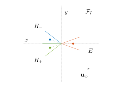
Figure 6: Relevant orbits of Eq. 35. Left: Phase space, switching manifolds (vertical dashed lines) and equilibria. Right: Sketch of equilibrium orientations of the sail.

In Fig. 6 we can see that the dynamics resembles that of a pendulum, where orbits librate around the sun-pointing orientation $E$. Concerning the stability of the equilibria, $H_{\pm}$ are unstable regardless of the values of the parameter. On the other hand, the the sun-pointing attitude $E$ is stable only if

$$k_{1,1}(\eta)>0\quad\Leftrightarrow\quad d> d_{\rm min}:=\frac{w(m_{b}+m_{s})}{2m_{b}}K(\alpha,\eta),$$ (36)

see Eq. 30. This has to be understood as a necessary condition for the stability of the sun-pointing attitude. Hence, we have justified the following result.

Proposition 1.

For each aperture angle $\alpha\in(0,\pi/2)$ and $\eta\in(0,1)$, if $d>d_{\rm min}$ as defined in Eq. 36 the sun-pointing direction $E$ is a locally stable equilibrium point of Eq. 35.

Note that as $K(\alpha,\eta)<0$, $d_{\rm min}<0$ and the attitude $E$ is stable, in particular, for all values $d>0$ and hence for all positions of the bus in front of the sail (e.g. all three sketches in Fig. 3), even beyond the tip of the sail. The value of $d_{\rm min}$ for $\alpha\in(0,\pi/2)$ is depicted in Fig. 7.

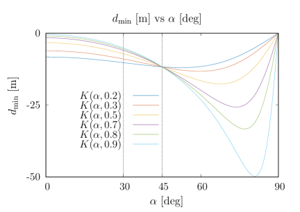
Figure 7: Depiction of the necessary condition for the stability of the sun-pointing attitude.

The motion restricted to $|\hat{\varphi}|<\alpha$, that physically corresponds to the case where both panels face sunlight (see Fig. 6 left, between the vertical dotted lines), is that of a mathematical pendulum. Even though Eq. 35 is only continuous, restricted to $|\hat{\varphi}|<\alpha$ the vector field is analytic. Thanks to this property one expects oscillations in this regime to persist for stronger gravity gradient effects, that is, for orbits that get closer to Earth surface, as classical averaging results apply in this region of the phase space, see LABEL:MC16.

4.1.2 Perturbation by gravity gradient

Here Eq. 31 without any assumption on $t_{\star}$ is considered. Recall that this consists of adding at the same time

1. The effect of the asymmetry of the body, that is a periodic behaviour whose period is that of the motion around the Earth, and

2. The period of rotation of the apparent motion of the Sun around the Earth.

In this situation, the invariant objects (equilibria, periodic orbits) of the system studied above in § 4.1.1 have their dynamically equivalent analogue in the 4D phase space of Eq. 31 under the conditions of smallness of $t_{\star}$, non-degeneracy and non-resonant conditions. These invariant objects have to be understood as if they“gained” the non-resonant frequencies of the perturbation [11]: e.g. under these hypotheses, the fixed point $E$ can have up to a 2-torus as dynamical substitute, and libration curve in Fig. 6 can have a 3-torus as dynamical substitute. But in this setting the existence of these objects can only be theoretically approached in $|\hat{\varphi}|<\alpha$ where the sail is equivalent to a pendulum and hence the vector field is analytic.

The relevance of these 3-tori is that as the phase space is 4D, these objects separate space and hence in case they exist they define a region where oscillations are perpetually bounded, and this orbits are strong candidates for practically bounded orbits in the complete system.

It is important to note that some of this structure is also expected to be destroyed due to the gravity gradient, that is, initial conditions in librational motion in the problem without gravity gradient can become eventually rotational once this effect is added. If the sail that is initially in $|\hat{\varphi}|<\pi-\alpha$ reaches $|\hat{\varphi}|>\pi-\alpha$ with nonzero angular velocity, this rotational state will never be lost. These kind of orbits are referred to as eventually tumbling. From a practical point of view, this defines an escaping criterion for simulations: the trajectory of an initial condition is discarded as tumbling if it reaches a state $|\hat{\varphi}|>\pi-\alpha$ with nonzero angular velocity before some prescribed integration time.

The smallness of the perturbation is key to be able to ensure the persistence of tori and hence the existence of stable attitude dynamics. Since we are assuming fixed Keplerian motion, we can write

$$r_{\rm sc}=\frac{a\sqrt{1-e^{2}}}{1+e\cos\theta},$$

Using this relation, the rightmost summand in Eq. 31d in Keplerian elements reads

$$P(\alpha,d)\frac{1}{a^{3}\sqrt{(1-e^{2})^{3}}}\gamma_{1}\gamma_{2}(1+e\cos\theta)^{3},\quad\mbox{where}\quad P(\alpha,d)=3\mu t_{\star}^{2}\frac{D(\alpha,d)}{C}.$$ (37)

How small the perturbation is depends on the values of $\alpha$ and $d$ via the factor $P(\alpha,d)$ in Eq. 37. The full dependence on these parameters is contained in the quotient $D(\alpha,d)/k_{1,1}(\eta)$, and it is easy to see that, for the values where $k_{1,1}(\eta)>0$, that is, when the orientation of the spacecraft towards the Sun is stable, for a fixed value of $\alpha$, as a function of $d$, the quotient (and hence $P(\alpha,d)$) is strictly convex and has an absolute minimum. In Fig. 8, left, we display some examples of $P(\alpha,d)$ for fixed values of $\alpha$.

Figure 8: Left: Size of the perturbation, $P(\alpha,d)$, see Eq. 37. Here we display curves for fixed $\alpha=10,20,30,40$ and $50$ deg. In the bottom left corner we indicate the corresponding value of our test example. Right: $P(30,0)/(R_{E}+a^{\prime})^{3}$, where $a^{\prime}$ is the altitude of the orbit.

In the right panel of Fig. 8 we display how does the perturbation size depend on the altitude of the orbit for ${\tt SC}_{1}$ and ${\tt SC}_{2}$. The vertical dashed lines indicate the separations from Low Earth Orbits (LEO) and Medium Earth Orbits (MEO) at $a^{\prime}=5000$ km, and between MEO and the geostationary region (GEO) at $a^{\prime}=35000$ km.

This shows that one has control on the size of the perturbation relying only on the physical parameters of the system, namely on the aperture angle $\alpha$ and the MPO $d$.

4.2 Bounded attitude motion: simplified versus complete model

Consider first the simplified model in Eq. 31. Under the presence of the gravity gradient torque, the dynamical objects of our interest are ideally replaced by tori of dimension and 3. These orbits appear, in a $\hat{\varphi}-\hat{\Phi}$ plot, as invariant curves around $E$. If such an orbit is detected, all initial conditions inside are attitude bounded. If instead one considers the attitude to affect the orbit, that is, to consider Eq. 26 instead of the simplification $\hat{M}^{\prime}=t_{\star}n$ (Eq. 31b) the formulation does not even provide a guess whether there would be or not any dynamical substitute, and in case there are, what is their dimension in the 6D phase space.

The purpose of this section is to provide numerical evidence of the existence of initial conditions that do not tumble before some large amount of time in the simplified model Eq. 31, and that some of this structure is actually seen in the full integration of Eq. 26.

4.2.1 Numerical experiment

Since the orbit dynamics is always transversal to the $x$ and $y$ axes, to detect such non-tumbling motion it is convenient to consider the hence well defined Poincaré section of Eq. 31 in

$$\Sigma=\{x=0,\;y<0\},$$ (38)

that is, in the negative $y$ axis, recall the sketch in Fig. 4. This reduces the problem to discrete and the dimension of the phase space by 1.

As the scope of this paper is the study of practically stable attitude dynamics, two orbit initial conditions are chosen: initially, ${\tt SC}_{1,2}$ are on an orbit with altitude $h_{0}=5000$ km, $\omega_{0}=0^{\circ}$ and $e=0.001$ or $0.1$. These are chosen to test the effect of stronger gravity gradient effects on the same spacecraft. An equispaced grid of 40 initial attitudes is chosen as follows

• For ${\tt SC}_{1}$, $\Phi_{0}=n_{\odot}$ rad/s and $\varphi_{0}=\lambda_{0}+0.9\times(180^{\circ}-30^{\circ})^{\circ}\times j/40$, $j=0,\ldots,39$,

• For ${\tt SC}_{2}$, $\Phi_{0}=n_{\odot}+2\times 0.9\times j/40$ rad/s, $j=0,\ldots,39$, $\varphi_{0}=\lambda_{0}$.

This segments have been chosen so that the most relevant parts of the phase space were visible in the $\hat{\varphi}-\hat{\Phi}$ plot. All initial conditions have been integrated for at most 1 year, and the integration was stopped before only in case along the orbit $|\hat{\varphi}|>\pi-\alpha$, that is, if the spacecraft started tumbling.

4.2.2 Numerical results

The $(\hat{\varphi},\hat{\Phi})$ components of the iterates of the Poincaré section to $\Sigma$ can be seen in Fig. 9 for ${\tt SC}_{1}$ and in Fig. 10 for ${\tt SC}_{2}$. In both figures, the left (resp. right) column show results for $e=0.001$ (resp. $e=0.1$). The top (resp. bottom) row shows results for the integration of the simplified (resp. complete) model. In all panels isolated dots are iterates of the Poincaré map that started tumbling before 1 year of integration.

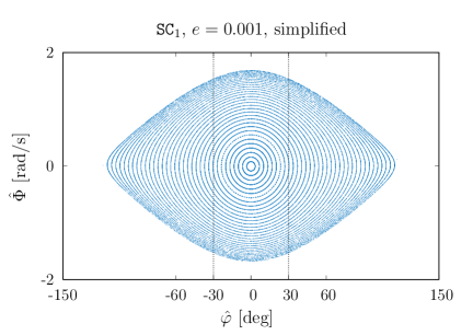
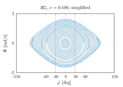
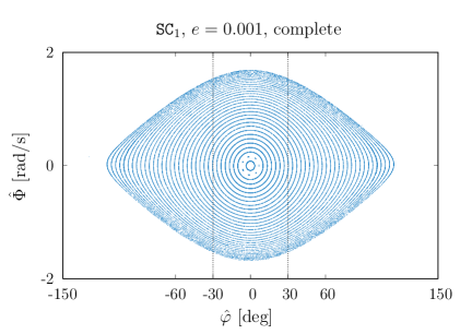
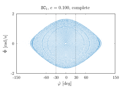
Figure 9: Iterates of the Poincaré map on $\Sigma$ of the initial condition described in § 4.2.1 for ${\tt SC}_{1}$. Top: simplified model. Bottom: complete model. Left: $e=0.001$. Right: $e=0.100$.

Concerning the results for ${\tt SC}_{1}$ in Fig. 9, the is a clear similarity between the attitude phase space of the simplified and complete model for both values of the initial eccentricity. This due to the fact that $d=0$ m for this spacecraft, and this is the most symmetric case possible for the class of spacecraft taken into account. But note that there are objects that appear in the phase space of the simplified model that are no longer there in the complete model and vice-versa. Compare the left panels, where orbits whose section seem to be periodic orbits close to the origin (sun-pointing attitude) both on top and in the bottom, but in different positions and with different periods. This can also be noticed in the right panels. Another feature that can be seen in the right panels is that while in the top figure there are what look like invariant curves, below it seems that orbits fill some are in the phase space. This is more prevalent in curves that are outside the $|\hat{\varphi}|<\alpha$ region, where oscillations are wider. There are many possible explanations of this observation. One possibility is that this is due to the chosen section, but it can also be caused either for the loss of differentiability of the vector field at $|\hat{\varphi}|=\alpha$, because these iterates belong to a bounded chaotic region, or even that these initial conditions diffuse to tumbling state, but for larger time scales.

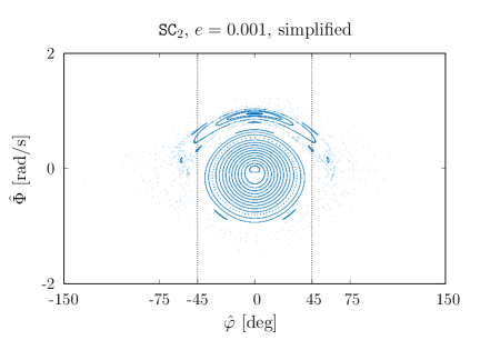
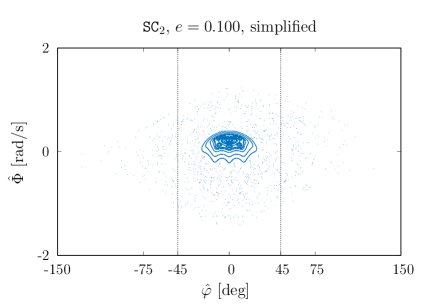
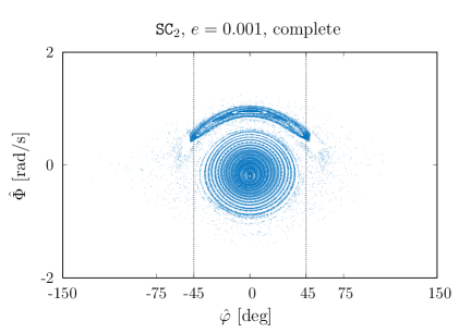
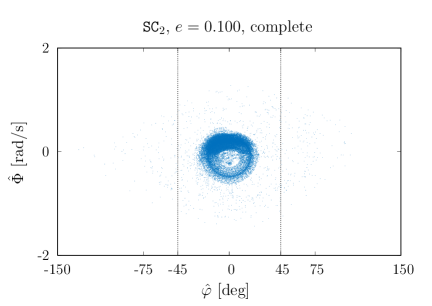
Figure 10: Iterates of the Poincaré map on $\Sigma$ of the initial condition described in § 4.2.1 for ${\tt SC}_{2}$. Top: simplified model. Bottom: complete model. Left: $e=0.001$. Right: $e=0.100$.

On the other hand, the results of the structure ${\tt SC}_{2}$ in Fig. 10 show that the displacement of the centre of mass has a huge impact on the region of stable oscillations. Most of these are confined in $|\hat{\varphi}|<\alpha$, where the vector field is analytic. On the left we see that the effect of the gravity gradient generated another equilibrium on top of the central region of oscillations, and some remnant of it is still visible in the iterates of the complete problem. In the right panels we see that for $e=0.100$ the region where there are stable oscillations is significatively reduced, and in fact for the complete problem only the initial conditions closest to the sun-pointing attitude reach 1 year without starting tumbling.

5 Attitude stability in a drag-dominated region

The torque and acceleration due to SRP and drag for the class of spacecraft under consideration are similar effects in the sense that the representations found in § 3.1.1 and § 3.1.2 are the same but the role played by the relative velocity vector in atmospheric drag is done by sunlight direction in SRP.

Despite this similarity, the two effects are different in nature as no reasonable simplifying assumptions - such as the apparent motion of the Sun being perfectly circular or $p_{\rm SR}$ being constant along the motion - can be done when studying atmospheric drag to get rid of the dependence on the position on the orbit the spacecraft is on. Namely, atmospheric drag depends explicitly on the orbit and on its position on it via the density $\rho$ and the modulus of the relative velocity $v_{\rm rel}$.

5.1 Some heuristic considerations

A simplified deterministic model as that provided in § 4.1 can not be given in this case, yet the whole coupled attitude and orbit model has to be tackled directly. Despite this, in light of the analysis performed in § 4.1, some heuristic considerations can be translated in this case to be able to draw a global description of the dynamics, qualitatively.

On the one hand, the expected rotation dynamics of the drag sail is expected to be oscillatory around the relative velocity vector, that now evolves as fast as the spacecraft orbits around the Earth. For attitude initial conditions sufficiently close to the orientation of the relative velocity vector, one expects that if a similar exploration as that in § 4.2.1 is performed, one could obtain an attitude phase space that is qualitatively similar to that in Fig. 6. In numerical simulations, one should plot $\hat{\phi}=\varphi-\delta=\varphi-\arctan(v_{y}/v_{x})$ as abscissa and $\Phi-{\rm d}\delta/{\rm d}t$ as ordinate. Note that we can provide an explicit expression for the latter, as

$$\frac{{\rm d}\delta}{{\rm d}t} = \frac{1}{v_{\rm rel}^{2}}\left(\frac{{\rm d}v_{y}}{{\rm d}t}v_{x}-\frac{{\rm d}v_{x}}{{\rm d}t}v_{y}\right),$$ (39)

where the derivatives of the components of the velocity are obtained by evaluating the orbit vector field.

On the other hand, concerning the position and stability of the attitude equilibria, one expects the relative velocity-pointing direction to be stable, generically, and that there is an analogous necessary stability condition related to that for SRP that reads as Eq. 36, but setting $\eta=0$. More concretely, the condition $k^{\prime}_{1,1}=k_{1,1}(0)>0$ is equivalent to

$$d> d_{\rm min}=\frac{w(m_{b}+m_{s})}{2m_{b}}K(\alpha,0).$$ (40)

The right hand side of Eq. 40 is depicted in Fig. 11, compare with Fig. 7.

Figure 11: Necessary conditions for the stability of the velocity-pointing orientation of the sail in drag-dominated regions.

Unlike in the SRP case, where the unstable $H_{\pm}$ were located at $\hat{\varphi}=\pm(\pi-\alpha$); if the sail is used as a drag sail, despite analogous orbits like $H_{\pm}$ exist, in the $(\varphi-\delta)-(\Phi-{\rm d}\delta/{\rm d}t)$ plane, their position depend on $\alpha$ and $d$. In particular, in case $d=0$ m, $k^{\prime}_{0,2}=k_{0,2}(0)=0$, see Eq. 23c and in that case $M_{0}(\pm\pi/2,0)=0$, recall Eq. 17. In this case $H_{\pm}$ are expected to be close to $(\pm\pi/2,0)$. In practice, this reduces the maximal range of oscillations that can be considered for each spacecraft, and has to be taken into account in simulations.

5.2 Bounded attitude motion

In this subsection the performance of the sails as depicted in Fig. 2 used as drag sails is tested. Unlike in the study of these structures as solar sails in § 4, where the goal was to find attitude initial conditions that remained close to the initial state for long periods of time, so that the average dynamics was as if the sail was flat and always pointing to the sunlight, in this case the problem has obvious boundaries and the performance can be measured in a well defined metric: if the motion starts at an initial altitude $h_{0}$, and one considers deorbiting as reaching a minimum value of the altitude $h_{\rm min}$, the best structure is the one that minimizes the time of flight.

5.2.1 Numerical experiment

As previously done in § 4.2.1, since the orbit is transversal to the axes of $\mathcal{F}_{I}$, the Poincaré section to $\Sigma$ (recall Eq. 38 and the sketch in Fig. 4) is considered.

To test and compare different structures in the same scenario a single orbit initial condition is considered: in all simulations the motion starts at the point $x=R+h_{0}$, $y=0$, where $R$ is the Earth’s radius and $h_{0}=600$ km is the initial altitude of the orbit. The orbit is assumed to be initially circular, so initially $\delta_{0}=\pi$ rad.

For this orbit initial condition, two illustrative numerical experiments have been performed: First, to look for stable attitude motion, an equispaced grid of 40 attitudes has chosen:

• For ${\tt SC}_{1}$, $\Phi_{0}={\rm d}\delta_{0}/{\rm d}t$ rad/s and $\varphi_{0}=\delta_{0}+0.5\times 90^{\circ}\times j/40$, $j=0,\ldots,39$,

• For ${\tt SC}_{2}$, $\Phi_{0}={\rm d}\delta_{0}/{\rm d}t$ rad/s and $\varphi_{0}=\delta_{0}+0.5\times 135^{\circ}\times j/40$, $j=0,\ldots,39$.

This is intended to study the performance as a function of the initial attitude condition.

The second experiment consists of a study of the performance of the structure as a function of the parameters $\alpha$ and $d$ of the structures. For each of the values of $\alpha=30^{\circ},40^{\circ},45^{\circ},50^{\circ},60^{\circ},70^{\circ}$ and $80^{\circ}$, two spacecraft have been considered: one with $d=0$, and another one assuming that the bus is at the tip of the sail, that is, for $d$ as given in Eq. 3. For each of these spacecraft, starting at the same orbit initial condition as in the first experiment, we have considered 40 attitude initial conditions, similarly chosen as

• For spacecraft with $d=0$ m, $\Phi={\rm d}\delta_{0}/{\rm d}t$ rad/s and $\varphi_{0}=\delta_{0}+0.5\times 90^{\circ}\times j/40$, $j=0,\ldots,39$,

• For spacecraft with the bus at the tip of the sail, $\Phi={\rm d}\delta_{0}/{\rm d}t$ rad/s and $\varphi_{0}=\delta_{0}+0.5\times(180^{\circ}-\alpha)\times j/40$, $j=0,\ldots,39$,

In all cases, ${\rm d}\delta_{0}/{\rm d}t$ is evaluated as in Eq. 39 and $h_{\rm min}=120$ km is considered.

The index $j$ of the attitude initial conditions is going to be used as label to identify them and to be able to compare results.

5.2.2 Numerical results

The results of the first experiment are summarized in Fig. 12. The left panels show the attitude iterates on $\Sigma$ of five initial conditions, those for $j=0,10,20,30$ and $39$. Only five initial conditions are displayed to be able to distinguish them easily. On the right, the evolution of the altitude from $h_{0}$ to $h_{\rm min}=120$ km for all the 40 initial conditions considered is displayed.

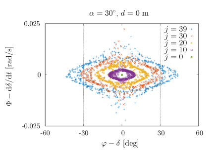
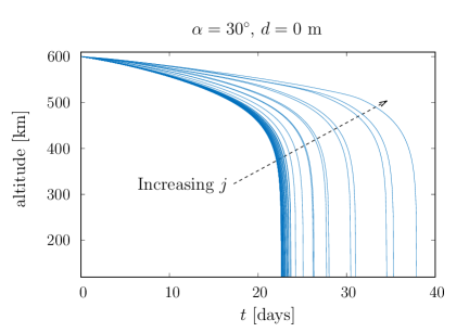
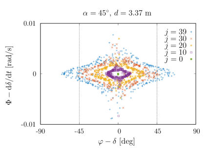
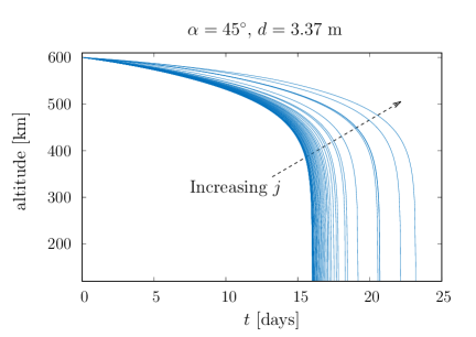
Figure 12: Left: Phase space of the Poincaré map on the section $\Sigma$ in the drag-dominated region. Right: Variation of the altitude of the orbit. Top: results for ${\tt SC}_{1}$. Bottom: results for ${\tt SC}_{2}$.

Concerning the attitude phase space in the left panels of Fig. 12, it is remarkable how, for both spacecraft, the initial condition $j=0$, that starts exactly at the relative velocity-pointing direction maintains this attitude with almost negligible variations at the displayed scale. The rest of initial conditions seem to fill an increasing area as time increases, in a tendency that seems to indicate slow diffusion towards a tumbling state. In both cases, the most robust initial conditions, meaning those whose range of $\varphi-\delta$ diffuses slowlier are those where the attitude is initially in an orientation in which both panels produce torque, that is, where $|\varphi-\delta|<\alpha$.

Concerning the deorbiting time, the displayed tendency shows that milder oscillations lead to faster deorbiting. Comparing the right column of Fig. 12 one sees that ${\tt SC}_{2}$ leads to faster deorbiting than ${\tt SC}_{1}$. The natural question whether this is due to the difference in parameter $\alpha$ or $d$ is answered with the second experiment.

In Fig. 13 the results of the preliminary sensitivity analysis are shown. On the left the results of spacecraft with $d=0$ m are shown, while on the right the bus is assumed to be at the tip of the spacecraft. In both cases one observes that, on the one hand, the larger $\alpha$ is (meaning closer to $90^{\circ}$), the faster the deorbiting is. In all cases, the larger $j$ (that is, the further one starts from the relative velocity-pointing attitude) the longer it takes to deorbit.

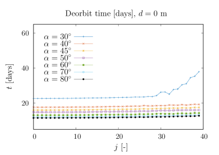
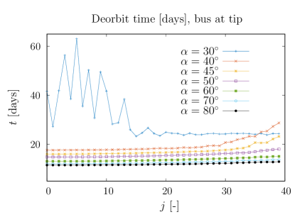
Figure 13: Deorbit time as a function of the initial condition (distance to velocity-pointing attitude) for different values of aperture angle $\alpha$. Left: $d=0$ m. Right: $d$ chosen to be in the tip of the sail, see Eq. 3.

Also, note that smaller values of $\alpha$ give worse performance as the amplitude of oscillations they can perform without starting tumbling is narrower. Finally, it is important to remark that for wider aperture angles $\alpha$ the value of $d$ does not seem to play a leading role as the deorbiting times are comparable. For instance, for $\alpha=80^{\circ}$, the deorbiting times almost coincide for small values of $j\leq 5$, with differences below 1 min, and for larger values of $j$ in the worst case the difference in performance for the two values of $d$ is of the order of 15 min.

6 Summary and conclusions

In this work a planar reduction of the coupled orbit and attitude dynamics of a solar/drag sail has been studied. The structures considered have a shape that endow them with auto-stabilizing properties: the sail structure consists of equal square panels in a way that form an angle $2\alpha$. Moreover, the position of the payload, and hence the mass distribution of the spacecraft, is put as a parameter, that measures the center of mass - center of pressure offset, and this is referred to as $d$.

One the one hand, helio-stability has been studied. The obtained results can be summarized as follows.

1. The stability of the sun-pointing attitude has been explicitly established as an analytic expression that involves the main parameters of the system: $\alpha$ and $d$. This can be used in practice as guideline for the construction of such spacecraft.

2. A further simplification of the problem allows to provide a model of the attitude motion that has Hamiltonian structure. In this model the dynamics has been shown to be pendulum-like close to the Sun-pointing direction and allows to measure explicitly regions of stability around this direction. These are, in fact, candidate attitude states to oscillate around the sunlight direction for large amounts of time in a complete problem taking into account more effects.

3. The numerical results of the simplified attitude model have been compared with numerical results of a coupled attitude and orbit system that takes into account the $J_{2}$ effect and the SRP acceleration of the oscillating sail. The better performance has been demonstrated to be for spacecraft with smaller $d$, that is, for cases in which the gravity gradient torque is smaller.

On the other hand, when dealing with the sail as a drag sail, there are no reasonable simplifying assumptions that allow to uncouple orbit and attitude dynamics. Hence the stability analysis performed in the SRP case cannot be directly translated into the drag case, yet some heuristic considerations can be done in light of the previous results. Namely, a similar guideline for how to choose $\alpha$ and $d$ so that the relative velocity-pointing direction is stable can be established.

This case has the advantage that the main interest is to deorbit rather than to maintain a concrete attitude, and the performance of the sails can be assessed by studying deorbiting times. The results in this case can be summarized as:

1. The stability of the relative velocity-pointing attitude has been numerically demonstrated. Here in all cases the best performance is in oscillatory motions where both panels produce torque (and hence acceleration) through the whole motion. Moreover, the smaller the amplitude of the oscillations, the faster deorbiting is.

2. The dependence of the deorbiting time on the parameters $\alpha$ and $d$ has been studied. The main conclusion has been that the closest $\alpha$ is to $\pi/2$ rad, the better, regardless of $d$ (prescribed it is chosen so that the velocity pointing attitude is stable).

The presented results provide evidence of the possibilities of considering non conventional sails such as the quasi-rhombic pyramid, as these lead to attitude oscillating stable dynamics if treated either a solar or a drag sail. The ranges of oscillation and the long term behaviour can be first approximated using simplified and easily treatable models. Concerning SRP, a long-term oscillating behaviour can be averaged out as done in [16], where this averaged dynamics was proven to be equivalent to considering a flat sail with fixed attitude towards the Sun. When drag is the main disturbance, if the initial state is sufficiently close to the relative velocity vector, the deorbiting time and trajectory can be well monitored as the attitude remains close to fixed. Similar results as those in [16] are expected to be obtained in light of the results exposed in this contribution, and will appear elsewhere.

There are a number of future lines of research that emerge from this work. The first and more natural one is to study the combined SRP and drag effects to deorbit satellites [17], but exploiting the auto-stabilizing properties of the family of sails under consideration to reduce as much as possible the need for attitude control. And of course the study of the dynamics and the performance of a 3D QRP as suggested in [2, 8], taking into account the effect of eclipses.

7 Acknowledgements

The research leading to these results has received funding from the Horizon 2020 Program of the European Union’s Framework Programme for Research and Innovation (H2020-PROTEC-2015) under REA grant agreement number 687500 – ReDSHIFT. The authors also acknowledge the ERC project COMPASS (Grant agreement No 679086), the use of the Milkyway High Performance Computing Facility and the associated support services at the Politecnico di Milano and the use of the computing facilities of the Dynamical Systems Group of Universiat de Barcelona. The datasets generated for this study can be found in the repository at the link www.compass.polimi.it/publications. The authors also thank fruitful conversations and support of J. Gimeno and M. Jorba-Cuscó.

References

- [1] J. A. Borja and D. Tun. Deorbit Process Using Solar Radiation Force. Journal of Spacecraft and Rockets, 43(3):685–687, 2006.
- [2] M. Ceriotti, P. Harkness, and M. McRobb. Variable-geometry solar sailing: the possibilities of quasi-rhombic pyramid. In M. McDonald, editor, Advances in Solar Sailing. Springer, 2013.
- [3] C. Colombo and T. de Bras de Fer. Assessment of passive and active solar sailing strategies for end of life re-entry. In International Astronautical Congress, number IAC-16-A6.4.4, 2016.
- [4] C. Colombo, C. Lücking, and C. R. McInnes. Orbital dynamics of high area-to-mass ratio spacecraft with and solar radiation pressure for novel earth observation and communication services. Acta Astronautica, 81:137–150, 2012.
- [5] C. Colombo, A. Rossi, F. Dalla Vedova, V. Braun, B. Bastida-Virgili, and H. Krag. Drag and Solar Sail deorbiting: re-entry time versus cumulative collision probability. In International Astronautical Congress, number IAC-17-A6.2.8, 2017.
- [6] F. Dalla Vedova, P. Morin, T. Roux, R. Brombin, A. Piccinini, and N. Ramsden. Interfacing Sail Modules for Use with “ Space Tugs ”. Aerospace, 5(48), 2018.
- [7] L. Felicetti, M. Ceriotti, and P. Harkness. Attitude Stability and Altitude Control of a Variable-Geometry Earth-Orbiting Solar Sail. Journal of Guidance, Control, and Dynamics, 39(9):2112 – 2126, 2016.
- [8] L. Felicetti, P. Harkness, and M. Ceriotti. Attitude and orbital dynamics of a variable-geometry, spinning solar sail in Earth orbit. In The Fourth International Symposium on Solar Sailing 2017 17th - 20th January, 2017, Kyoto, Japan, pages 1–10, 2017.
- [9] H. Goldstein and C.P. Poole. Classical Mechanics. Addison-Wesley series in Physics. Addison-Wesley Publishing Company, 1980.
- [10] L. Johnson, M. Whorton, A. Heaton, R. Pinson, G. Laue, and C. Adams. Nanosail-D: A solar sail demonstration mission. Acta Astronautica, 68(5):571 – 575, 2011. Special Issue: Aosta 2009 Symposium.
- [11] À. Jorba and J. Villanueva. On the persistence of lower dimensional invariant tori under quasi-periodic perturbations. Journal of Nonlinear Science, 7, 10 1997.
- [12] M. Jorba-Cuscó, A. Farrés, and À. Jorba. Periodic and quasi-periodic motions for a solar sail in the Earth-Moon system. Proceedings of the International Astronautical Congress, IAC, pages 1–11, 2016.
- [13] C. Lücking, C. Colombo, and C. R. McInnes. A passive satellite deorbiting strategy for MEO using solar radiation pressure and the effect. Acta Astronautica, 77:197–206, 2012.
- [14] C. Lücking, C. Colombo, and C. R. McInnes. Solar radiation pressure-augmented deorbiting: Passive end-of-life disposal from high-altitude orbits. Journal of Spacecraft and Rockets, 50, 11 2013.
- [15] F.L. Markley and J.L. Crassidis. Fundamentals of Spacecraft Attitude Determination and Control. Space Technology Library. Springer New York, 2014.
- [16] N. Miguel and C. Colombo. Attitude and orbit coupling of planar helio-stable solar sails. arXiv e-prints, page arXiv:1904.00436, Mar 2019.
- [17] V. Stolbunov, M. Ceriotti, C. Colombo, and C. R. McInnes. Optimal Law for Inclination Change in an Atmosphere Through Solar Sailing. Journal of Guidance, Control, and Dynamics, 36(5):1310 – 1323, 2013.
- [18] Y. Tsuda, O. Mori, R. Funase, H. Sawada, T. Yamamoto, T. Saiki, T. Endo, and J. Kawaguchi. Flight status of IKAROS deep space solar sail demonstrator. Acta Astronautica, 69(9):833 – 840, 2011.