Resonance–Assisted Tunneling in Deformed Optical Microdisks
with a Mixed Phase Space

Abstract

The life times of optical modes in whispering-gallery cavities crucially depend on the underlying classical ray dynamics and may be spoiled by the presence of classical nonlinear resonances due to resonance–assisted tunneling. Here we present an intuitive semiclassical picture which allows for an accurate prediction of decay rates of optical modes in systems with a mixed phase space. We also extend the perturbative description from near-integrable systems to systems with a mixed phase space and find equally good agreement. Both approaches are based on the approximation of the actual ray dynamics by an integrable Hamiltonian, which enables us to perform a semiclassical quantization of the system and to introduce a ray-based description of the decay of optical modes. The coupling between them is determined either perturbatively or semiclassically in terms of complex paths.

I Introduction

Optical microcavities allow for a wide range of applications Vah2004 ; CaoWie2015 in, for instance, sensors ForSwaVol2015 and lasing devices HeOezYan2013 . Optical modes with long life times and directional emission properties are desired. Long life times, and thus also large quality factors, are realized by whispering–gallery cavities in which light is confined by almost total internal reflection. This is achieved by a circular or spherical cavity design for which the classical ray dynamics is integrable. In contrast, directional emission is achieved by deforming the cavities boundary from the perfectly circular or spherical shape and thus rendering the classical ray dynamics nonintegrable NoeStoCheGroCha1996 ; WieHen2008 . In quasi two-dimensional cavities classical whispering–gallery trajectories persist under sufficiently small and smooth deformations. This, in general, gives rise to the coexistence of regular and chaotic ray dynamics in a mixed phase-space Laz1973a . While the associated whispering–gallery modes are still present in the deformed cavity, their quality factors get spoiled, i.e., their life times decrease.

One major mechanism causing this enhanced decay is the wave effect of dynamical tunneling which was first observed and extensively studied in quantum systems DavHel1981 ; KesSch2011 . More recently it has been studied both theoretically and experimentally in microwave resonators DemGraHeiHofRehRic2000 ; BaeKetLoeRobVidHoeKuhSto2008 ; DieGuhGutMisRic2014 ; GehLoeShiBaeKetKuhSto2015 and optical microcavities HacNoe1997 ; PodNar2005 ; BaeKetLoeWieHen2009 ; ShiHarFukHenSasNar2010 ; ShiHarFukHenSunNar2011 ; YanLeeMooLeeKimDaoLeeAn2010 ; KwaShiMooLeeYanAn2015 ; YiYuLeeKim2015 ; YiYuKim2016 ; ShiSchHenWie2016 ; KulWie2016b ; YiKulKimWie2017 . Dynamical tunneling allows for coupling of optical modes associated with dynamically separated classical phase-space regions. Specifically, long living whispering–gallery modes may couple to faster decaying modes via dynamical tunneling. In particular, classical nonlinear resonances in the ray dynamics may drastically enhance tunneling effects by the mechanism of resonance–assisted tunneling BroSchUll2002 . Again the majority of theoretical understanding has been obtained in quantum systems, e.g., quantum maps BroSchUll2001 ; BroSchUll2002 ; EltSch2005 ; LoeBaeKetSch2010 ; SchMouUll2011 . Recent experiments, however, have impressively demonstrated the effect also in microwave resonators GehLoeShiBaeKetKuhSto2015 and in two-dimensional optical microcavities KwaShiMooLeeYanAn2015 . While the latter qualitatively follows the theoretical description of resonance–assisted tunneling obtained in quantum maps a quantitative description of resonance assisted tunneling in optical microcavities has been given only recently for systems with near-integrable ray dynamics KulWie2016b ; YiKulKimWie2017 . For this, the classical ray dynamics has been approximated by a pendulum-like Hamiltonian, which subsequently allows for the perturbative expansion of optical modes and their quality factors as predicted by resonance–assisted tunneling. Moreover, this description has been shown to capture the enhanced decay of optical modes correctly in situations when the perturbative scheme developed in Ref. DubBogDjeLebSch2008 fails. Nevertheless, the prediction based on resonance–assisted tunneling has two major limitations. On the one hand it depends on the circular cavity yielding a good approximation of the actual ray dynamics in order to construct the approximating pendulum Hamiltonian. This will not be accurate for larger deformations of the cavitiy boundary. On the other hand for larger deformations also the optical modes of the circular cavity will no longer provide a suitable unperturbed basis for the perturbative treatment.

In this paper we extend the perturbative description of resonance–assisted tunneling in optical microcavities to systems with a mixed phase space. In addition, we apply the semiclassical description of resonance–assisted tunneling which leads to a simple and intuitive picture. To this end, based on an idea presented in Ref. RobBer1985 , we introduce a suitable coordinate system and subsequently construct the approximating pendulum Hamiltonian. These coordinates further allow for semiclassical Einstein–Brillouin–Keller (EBK) quantization of the system KelRub1960 ; NoeSto1997 ; Noe1997 . This enables us to compute wave numbers as well as their associated classical phase-space structures. Moreover, this provides the unperturbed basis necessary for the perturbative treatment and thus allows for the construction of couplings between modes due to resonance–assisted tunneling. We further use both the approximating pendulum Hamiltonian and the semiclassical EBK quantization scheme to obtain a semiclassical description of these couplings. Combining the coupling of different modes with a ray-based model for their decay finally allows to accurately describe the complex wave numbers and thus the decay of optical modes in the presence of resonance–assisted tunneling. Both the semiclassical and perturbative description agree well with numerical solutions of the mode equation.

This paper is organized as follows: In Sec. II we introduce deformed optical microdisks. We study their classical ray dynamics in Sec. II.1 and introduce the full wave picture in terms of the mode equation in Sec. II.2. In Sec. II.3 we discuss numerical solutions to the mode equations and briefly review a perturbative approach and its applicability to resonance–assisted tunneling in Sec. II.4. Sec. III introduces the basic concepts of our description. This includes the introduction of adiabatic action angle coordinates in Sec. III.1 and the subsequent construction of an approximating pendulum Hamiltonian in Sec. III.2. The semiclassical quantization scheme is discussed in Sec. III.3 and a ray-based model for the decay of optical modes is introduced in Sec. III.4. Finally, Sec. III.5 contains the perturbative description of resonance–assisted tunneling while the semiclassical picture is presented in Sec. III.6. A summary and outlook are given in Sec. IV.

II Deformed Optical Microdisks

In this section we introduce deformed optical microdisks and present the model systems studied in this paper. We discuss their classical ray dynamics as well as solving Maxwells equations to obtain the optical modes and their decay rates.

II.1 Ray Dynamics

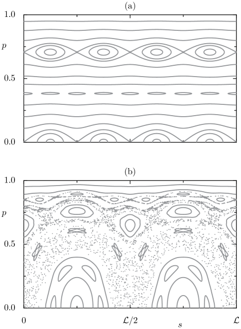
Figure 1: (a) Phase space of the near-integrable system and (b) phase space of the mixed system with parameters given in the text. Regular tori are depicted by lines, while dots correspond to chaotic orbits.

The classical ray dynamics of a cavity is given by light rays traveling on straight lines inside the cavity and specular reflections at the boundary. Thus the dynamics is completely determined by the positions of the bounces on the boundary and the angle $\chi$ of the reflected ray with the inwards normal vector of the boundary. Therefore the dynamics can be completely described in Birkhoff coordinates $(s,p)$, where $s$ denotes the arc length along the boundary ranging from $0$ to the full boundary length $\mathcal{L}$ and $p=\sin(\chi)$ is the canonically conjugate momentum. In Birkhoff coordinates, the dynamics is conveniently represented in the phase space $(s,p)\in\left[0,\mathcal{L}\right]\times\left[-1,1\right]$ by a symplectic map $(s,p)\mapsto(s^{\prime},p^{\prime})$ given by successive bounces and the corresponding momenta.

Typically, the dynamics generated by this map will be nonintegrable, as the full system has two degrees of freedom while there is no second conserved quantity besides energy. In fact, there are only a few cavities with integrable ray dynamics and smooth boundary. Among them, the circular cavity is the most simple case. However, a generic deformation of a circular boundary will render the ray dynamics nonintegrable. Typically, with growing deformation the dynamics will change from near integrable for small deformations towards a mixed phase space for larger deformations. For even larger deformations the dynamics can become fully chaotic. An important exception is the elliptic cavity, in which the eccentricity can be seen as deformation parameter. There, the ray dynamics remains integrable independent of the eccentricity and thus even for large deformations. The boundary of a deformed circular cavity can be described by its radial coordinate $r$ as a function of the polar angle $\varphi$. For cavities with reflection symmetry with respect to an axis and with smooth boundaries this function can be written as a Fourier series, $r(\varphi)=R\left(1+\sum_{j\geq 1}d_{j}\cos(j\varphi)\right)$, with mean radius $R$. As concrete examples we will consider cases where only one of the coefficients $d_{N}:=\epsilon$ is nonzero, i.e.,

$$r(\varphi)=R\left(1+\epsilon\cos(N\varphi)\right).$$ (1)

In particular we choose $R=1$, $\epsilon=0.0025$ and $N=4$ as an example of a weakly deformed cavity with near-integrable ray dynamics which was also considered in Ref. KulWie2016b . Its phase space, shown in Fig. 1(a), is predominantly foliated by invariant tori. At $p=0$ there are two stable and two unstable period-two orbits, which correspond to trajectories along the diameter of the cavity. In phase space this periodic motion leads to orbits consisting of only two points each. It can be characterized by a frequency $\omega=\mathcal{L}/2$, by which the arc-length coordinate advances in between successive bounces. The periodicity of these orbits is reflected by the fact that this frequency fulfills a resonance condition, i.e., it is a rational multiple of $\mathcal{L}$. Therefore one has

$$\omega=\omega_{a:b}=b\mathcal{L}/a$$ (2)

for integers $a$ and $b$. The period of the orbits is given by the numerator of $a/b$ after fully reducing this fraction. In phase space this gives rise to a chain of $a$ eye-like structures, called a nonlinear resonance. The frequency $\omega_{a:b}$ is such, that the central periodic orbits within these resonance eyes advance by $b$ eyes in between successive bounces. Thus, for the two pairs of stable and unstable period-two orbits, a $a:b=4:2$ resonance chain arises in phase space. It is bounded by a very thin chaotic layer, which can not be distinguished from regular tori at the shown scale. In addition a large $4:1$ resonance occurs around $p_{4:1}=\cos(\pi/4)=1/\sqrt{2}$. For larger momenta $p\to 1$ again motion along regular tori dominates the phase-space portrait. In configuration space the corresponding trajectories closely follow the boundary of the cavity and are therefore called whispering–gallery trajectories. Their existence is guaranteed by a theorem of Lazutkin Laz1973a if the curvature of a smooth boundary is bounded from below and above by some positive constants. As the deformation parameter $\epsilon$ is small the shape of the boundary does not deviate much from the circular cavity. Thus the regular dynamics of the circular cavity approximates the motion along regular tori of the weakly deformed system well.

Another example we consider is given by $R=1$, $\epsilon=0.08$ and $N=2$. This deformation is called quadrupol deformation and, although the deformation parameter $\epsilon$ is again small compared to unity, it gives rise to a mixed phase space as it is shown in Fig. 1(b). Hence, in the following we will use the shorthand notion of a mixed system for this example. For small momenta the phase space is governed by the regular islands around the stable period-two orbit and the chaotic regions around the unstable period two-orbit at $p=0$. For large momenta, $|p|$ close to $1$, again Lazutkins theorem implies the existence of regular motion along invariant tori which correspond to whispering–gallery trajectories in configuration space. Below the last invariant torus a large $4:1$ resonance occurs around $p_{4:1}=1/\sqrt{2}$. More precisely, the unstable period-four orbit has constant momentum $p_{4:1}$, while its stable counterpart oscillates around this value. This $4:1$ nonlinear resonance chain is surrounded by a partial barrier as manifested by different densities of points in the chaotic region in Fig. 1(b). Inside the chaotic regions smaller nonlinear resonances of order proportional to $N=2$ can be found.

The quadrupol deformation agrees in lowest order of the deformation parameter with the elliptical cavity. That is, the boundary of the elliptic cavity with eccentricity $\epsilon_{\mathrm{ecc}}$ in polar coordinates can be written as

$$r(\varphi)=\frac{R\sqrt[4]{1-\epsilon_{\mathrm{ecc}}^{2}}}{\sqrt{1-\epsilon_{\mathrm{ecc}}^{2}\cos^{2}(\varphi)}},$$ (3)

which for small $\epsilon_{\mathrm{ecc}}$ can be expanded as YiKulKimWie2017

$$r(\varphi)\approx R\left(1+\epsilon\cos(2\varphi)\right).$$ (4)

Here $\epsilon$ and the eccentricity $\epsilon_{\mathrm{ecc}}$ are related via

$$\epsilon_{\mathrm{ecc}}=\sqrt{1-(1-\epsilon)^{4}}.$$ (5)

Thus the motion along regular tori corresponding to whispering-gallery trajectories in the mixed system can be approximated by the regular dynamics of the elliptic cavity with eccentricity given by Eq. (5).

As the billiard-like dynamics inside a cavity corresponds to the classical ray picture of optics it is expected to be valid only in the limit of vanishing wave length or equivalently large wave numbers $k$. For smaller wave numbers semiclassical corrections to the classical ray picture may become relevant. Most famous among these corrections is the so-called Goos–Hänchen shift GooHae1947 ; Art1948 . It describes the deplacement between the center of an incoming light beam and the center of the reflected beam. In particular, this causes the position of periodic orbits and the associated nonlinear resonance chain to undergo a shift in momentum UntWie2010 . This periodic-orbit shift is given by UntWie2010 ; KulWie2016b

$$\Delta p_{\mathrm{POS}}(k)=\frac{p_{a:b}}{R_{\mathrm{c}}\mathrm{Re\,}k\sqrt{n^{2}p_{a:b}^{2}-1}},$$ (6)

where $p_{a:b}=\cos(b\pi/a)$ for an $a:b$ resonance. Here, $n$ denotes the refractive index inside the cavity and $R_{\mathrm{c}}$ is the average of the radii of curvature of the boundary taken over all points of the stable and unstable periodic orbit. Equation (6) will be used in the following, when comparing classical phase-space structures with solutions of Maxwells equations.

II.2 Mode Equation

While the classical dynamics inside the cavity is governed by light rays traveling along straight lines and undergoing specular reflections at the boundary, the electro–magnetic field is described by Maxwells equations in full space. Solutions to Maxwells equations with harmonic time dependence $\propto e^{\mathrm{i}\omega t}$ in a quasi two-dimensional cavity fulfill the mode equation

$$\Delta\psi(\mathbf{r})+n({\mathbf{r}})^{2}k^{2}\psi({\mathbf{r}})=0$$ (7)

in combination with appropriate boundary conditions. Here, $k=\omega/c$ denotes the wave number while $c$ is the speed of light in vacuum. The effective refractive index $n({\mathbf{r}})$ in Eq. (7) is considered to be constant, $n({\mathbf{r}})=n$, inside the cavity and is set to unity on the outside in the following. For numerical calculations we use $n=2$. Depending on the polarization the optical mode $\psi(\mathbf{r})$ corresponds to either the component perpendicular to the cavity plane of the electric field, which is called transversal magnetic (TM) polarization, or of the magnetic field, called transversal electric (TE) polarization. For TM polarization $\psi$ and its normal derivatives are continuous at the cavities boundary. While we will focus on TM polarized light, we expect the results of this paper to be applicable also in the TE case when the appropriate boundary conditions are applied. Requiring also outgoing wave boundary conditions at infinity, i.e., an asymptotic behavior $\text{e}^{\mathrm{i}kr}/\sqrt{r}$ for large $r$, Eq. (7) has solutions only for discrete complex wave numbers with negative imaginary part. If the boundary of the cavity exhibits reflection symmetry along an axis, the optical modes reflect that symmetry, i.e., they fulfill either Dirichlet or Neumann boundary conditions on that symmetry axis. Thus in the cavities under consideration, which are symmetric with respect to both horizontal and vertical axis, the optical modes are grouped into four symmetry classes.

By means of semiclassical quantization in classically integrable or mixed systems at least some of the possible modes and their mode numbers $k=k_{ml}$ are labeled by an angular mode number $m$ and a radial mode number $l$. In particular modes with small radial mode number $l$ are associated with whispering–gallery trajectories and thus are called whispering–gallery modes. As the wave numbers are complex the intensity of optical mode inside the cavity decays as $\text{e}^{-\Gamma_{m,l}t}$ with a decay rate $\Gamma_{m,l}=-2c\,\mathrm{Im}\,k_{m,l}$, which is exponentially small for whispering–gallery modes and thus corresponds to large life times $\tau_{m,l}=1/\Gamma_{m,l}$. This is often also quantified by the quality factor $Q_{m,l}=-\mathrm{Re}\,k_{m,l}/(2\mathrm{Im}\,k_{m,l})$. As for both decay rates and for quality factors it is sufficient to determine the wave numbers $k_{m,l}$ we will focus on these in the following. In particular, we study whispering–gallery modes with fixed radial quantum number $l=0$.

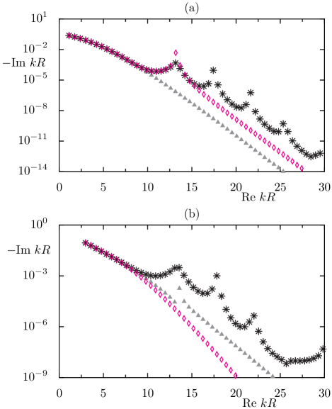
Figure 2: Wave numbers for whispering–gallery modes with $l=0$ (a) for the near-integrable system starting from $m=1$ and (b) for the mixed system starting from $m=4$ as black stars. The wave numbers of the integrable counterpart, i.e., (a) the circular cavity and (b) the elliptic cavity are shown as gray triangles. The perturbative prediction, Eq. (9), is depicted by open magenta diamonds.

II.3 Numerical Results

An analytical solution to Eq. (7) and for the wave numbers $k_{m,l}$ is only known for the circular cavity. Therefore in general numerical or approximate schemes have to be used. A standard numerical approach both for closed billiards and cavities is the boundary element method (BEM) Bae2003 ; Wie2003 , which we combine with the ideas of Ref. Kre1991 to gain the required accuracy for the exponentially small imaginary wave numbers. We use this approach to determine the dimensionless wave numbers $Rk_{m,l}$ for whispering gallery modes with mode numbers $(m,l=0)$ in the near-integrable system and the mixed system. They are shown as black stars in Fig. 2 for the (a) near-integrable and (b) mixed system. There, $-\mathrm{Im}\,k_{m,l}R$ is depicted semilogarithmically as a function of $\mathrm{Re}\,k_{m,l}R$. This representation is usually employed for decay rates in quantum maps plotted against the inverse semiclassical parameter, whose role is played by $\mathrm{Re}\,k_{m,l}R$ in our case, and is well suited to study resonance–assisted tunneling. We focus on modes which fulfill Dirichlet boundary conditions on the horizontal symmetry axis. Modes with even angular mode number $m$ additionally fulfill Dirichlet boundary conditions along the vertical symmetry axis, while for odd $m$ they fulfill Neumann boundary conditions. The wave numbers of modes belonging to other symmetry classes show qualitatively the same behavior and cannot be distinguished from the depicted data on the shown scale. For small $\mathrm{Re}\,k_{m,l}R$ the imaginary parts follow an exponential decay, which is equal to the wave numbers of its integrable counterpart, i.e., the circular and elliptic cavity, respectively. Their wave numbers are shown as gray triangles and are computed analytically for the circular cavity and numerically using the BEM for the elliptic cavity. Note, that for the elliptic cavity the imaginary parts of the wave numbers do not show a pure exponential decay as there are deviations around $\mathrm{Re}\,k_{m,l}R=13$. This is expected to be due to the open boundary condition of optical cavities YiKulKimWie2017 . However, for both the near-integrable and the mixed system, at some point the imaginary parts of the wave numbers deviate from the integrable case due to resonance–assisted tunneling induced by the $4:1$ resonance. There is still an overall exponential decay which is similar to the exponential decay observed in the integrable case. This overall decay is accompanied by peaks, at which the negative imaginary part of the wave number is enhanced by roughly two orders of magnitude. While showing qualitatively similar behavior, the overall exponential decay is slower in the case of the mixed system. In the mixed system the overall exponential decay and the peak structure are present only up to wave numbers with $\mathrm{Re}\,k_{m,l}R=25$. For larger real parts of the wave numbers their imaginary parts start to form a plateau and even increase towards $\mathrm{Re}\,k_{m,l}R=30$. Similar effects have been observed in the studies on resonance–assisted tunneling in quantum maps if additional smaller resonances become important LoeBaeKetSch2010 . In the near-integrable system this plateau formation is not observed in the investigated regime of wave numbers.

A qualitative idea of the mechanism causing the peaks for specific values of $\mathrm{Re}\,k_{m,l}R$ can be obtained from the intensity $|\psi(\mathbf{r})|^{2}$ of the optical modes shown in Fig. 3. Here the intensity is shown for the mode with $m=27$ for the near-integrable system in Fig. 3(a) and with $m=28$ for the mixed system in (b) which corresponds to modes in between the first two peaks. In both cases the region of largest intensity basically follows the boundary of the cavity resembling classical whispering–gallery trajectories. Closer inspection reveals that the shape of the rectangular stable period-four orbit also influences the morphology of the intensity patterns. In contrast, the modes corresponding to the first peak are shown in Fig. 3(c) for the near-integrable system with $m=22$ and in (d) for the mixed system with $m=23$. Both appear as a superposition of modes with different radial mode numbers. In the near-integrable system the admixture of modes with larger radial mode number $l>0$ is well seen in the regions where the stable period four orbit hits the boundary. In the mixed system a similar pattern emerges where the unstable period-four orbit hits the boundary.

The above observations are also reflected in the phase-space representation of the modes. To this end we also show the incident Husimi function HenSchSch2003 on the inside of the boundary in Fig. 3 superimposed on the classical phase space. The Husimi functions are obtained from the overlap of $\psi$ and its normal derivative with Gaussian coherent states defined on the boundary. We choose the ratio of their uncertainties in $s$ and $p$ to be equal to the boundary length $\mathcal{L}$ in order to increase the resolution in $p$ direction and to take the extent of phase space in both $s$ and $p$ into account. Doing so we find the mode with $m=27$ in the near-integrable system to localize well above the $4:1$ resonance and to match the shape of the regular tori as shown in Fig. 4(a). Similarly, in the mixed system the mode with $m=28$ shown in (b) localizes above the $4:1$ resonance where it follows the shape of adiabatically invariant curves, see Fig. 5(a).

The localization properties of the modes with $m=22$ in the near-integrable system and with $m=23$ in the mixed system shown in Fig. 4(c) and (d), respectively, exhibit a different morphology. They predominantly localize on the $s$-coordinates of either the stable period four orbit in the near-integrable system or of the unstable period-four orbit in the mixed system. However, in $p$ direction the modes are shifted upwards compared to the $p$ coordinates of the respective period-four orbits. This is due to the periodic-orbit shift, Eq. (6). Incorporating this shift would lead to the modes localizing predominantly on the stable periodic orbit in the near-integrable system and on the unstable periodic orbit in the mixed system, respectively (not shown). Besides the regions of maximal intensity along the periodic orbits there are additional phase-space regions with significant intensity. This is most clearly seen in Fig. 4(c) for the near-integrable system. In this case these regions correspond to two regular tori located above and below the, according to Eq. (6) appropriately shifted, $4:1$ resonance. Taking again the periodic-orbit shift into account would result in those tori being located symmetrical with respect to the resonance. Thus the mode with $m=23$ may be interpreted as a superposition of modes localizing on these two different classical tori. In the mixed system the regions with additional intensity are located on either side of the $4:1$ resonance as well. Above the resonance chain this contribution shows a similar morphology as the mode with mode number $m=28$. In contrast, the contribution below the resonance chain resembles the shape of the partial barrier associated to the $4:1$ resonance. Note, that this contribution looks quite regular despite the absence of regular tori in this phase space region.

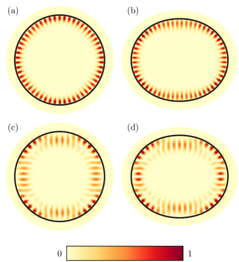
Figure 3: The intensity patterns with the respective maximum intensity normalized to unity for the modes with (a) $m=27$ and (c) $m=22$ for the near-integrable systems and (b) $m=28$ and (d) $m=23$ for the mixed system are shown. The black line represents the boundary of the respective cavity.

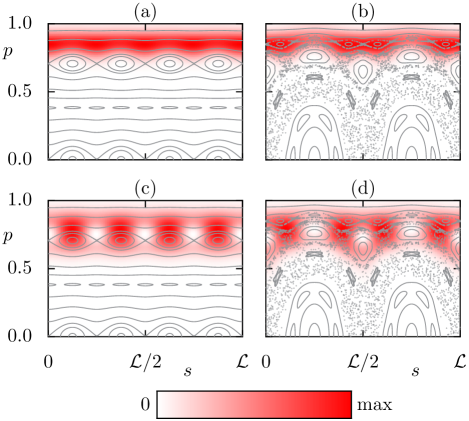
Figure 4: The incident Husimi representation of the modes with (a) $m=27$ and (c) $m=22$ for the near-integrable systems and (b) $m=28$ and (d) $m=23$ for the mixed system are superimposed on the classical phase space shown in gray.

II.4 Perturbation Theory

In addition to the numerical solutions of the mode equation (7) also approximate solutions can be obtained. In particular the perturbative expansion of optical modes and wave numbers $k_{m,l}$ in the deformation parameter $\epsilon$ has proven to yield good agreement with numerical results for sufficiently small deformation DubBogDjeLebSch2008 . For this approach the modes and wave numbers $\tilde{k}_{m,l}$ of the circular cavity provide the unperturbed basis. For TM polarized light and angular mode number $m$ the latter are computed as the roots of DubBogDjeLebSch2008

$$S_{m}(\tilde{k}R)=n\frac{J^{\prime}_{m}(n\tilde{k}R)}{J_{m}(n\tilde{k}R)}\ -\frac{H^{\prime}_{m}(\tilde{k}R)}{H_{m}(\tilde{k}R)}.$$ (8)

Here, $J_{m}$ and $J^{\prime}_{m}$ as well as $H_{m}$ and $H^{\prime}_{m}$ denote Bessel and Hankel functions of the first kind and of order $m$ and their derivative, respectively. The radial mode number $l$ corresponds to the $l$-th root of $S_{m}$ when ordered by ascending real part. The wave numbers in second order perturbation theory for deformations of the type of Eq. (1) are given by DubBogDjeLebSch2008 ; KulWie2016b

$$k_{m,l}= \tilde{k}_{m,l}-\frac{\epsilon^{2}}{4}\tilde{k}_{m,l}\left(1+2\tilde{k}_{m,l}\frac{H^{\prime}_{m}}{H_{m}}\right)$$

$$-\frac{\epsilon^{2}}{4}(n^{2}-1)\tilde{k}_{m,l}^{2}\left(\frac{1}{S_{m+N}}+\frac{1}{S_{m-N}}\right),$$ (9)

if $m>N$. Here, $S_{m\pm N}$, $H_{m}$ and $H_{m}^{\prime}$ are evaluated at $\tilde{k}_{m,l}R$. Only the last term contains the coupling of modes with different angular mode numbers differing from $m$ by $\pm N$. The contribution to the imaginary part $\mathrm{Im\,}\delta k_{m,l}^{(\pm N)}$ caused by these mode couplings is given by DubBogDjeLebSch2008

$$\mathrm{Im\,}\delta k_{m,l}^{(\pm N)}=-\epsilon^{2}\frac{(n^{2}-1)\mathrm{Re\,}\tilde{k}_{m,l}}{2\pi|S_{m\pm N}H_{m\pm N}|^{2}}.$$ (10)

Therefore, in the perturbative framework enhancement of the negative imaginary part may occur if $S_{m\pm N}(\tilde{k}_{m,l}R)$ becomes small. This, however, corresponds to $\tilde{k}_{m,l}$ being almost degenerate with a mode of angular quantum number $m\pm N$. As we study modes with $l=0$ and $\mathrm{Re\,}k_{m,0}<\mathrm{Re\,}k_{m+N,0}$ holds, this degeneracy is only possible between modes with mode numbers $(m,0)$ and $(m-N,\tilde{l})$ for some $\tilde{l}>0$. Thus $\mathrm{Im\,}\delta k_{m,l}^{(-N)}$ may cause the peaks seen in Fig. 2 in the numerically obtained wave numbers. There the perturbatively obtained wave numbers for both the near-integrable and the mixed system are shown as open magenta diamonds in Fig. 2(a) and (b), respectively. In both cases they give rise to the correct initial exponential decay of $\mathrm{Im}\,k_{m,l}R$. In the near-integrable system perturbation theory accurately predicts the first peak but fails to describe the second peak. In contrast for the mixed system the perturbative description fails to describe even the first peak. This failure can be traced back to coupling between modes whose angular mode numbers differ by $\pm N$. In the following sections we will argue that the relevant couplings occur between modes whose angular mode numbers differ by multiples of the order $a=4$ of the relevant $4:1$ resonance. In the near-integrable system we have $a=N$ and thus second order perturbation theory resolves the first peak. In contrast in the mixed system we have $a=2N$ and thus second order perturbation theory fails to explain the first peak. Additional couplings appear in higher orders of perturbation theory only. Whether or not they give rise to additional peaks is so far an open question, which will not be discussed here.

III Ressonance–Assisted Tunneling

In the following we derive the framework which allows for a perturbative as well as a semiclassical description of complex wave numbers in optical microcavities. To this end we construct a canonical transformation from Birkhoff coordinates $(s,p)$ to adiabatic action–angle coordinates $(S,P)$. In these coordinates the dynamics in the vicinity of the relevant nonlinear resonance can be approximated by an integrable pendulum-like Hamiltonian. In addition the adiabatic action coordinates allow for EBK quantization of the full system, which establishes a connection between wave numbers $k_{m,l}$ and quantizing adiabatic actions $P_{m,l}$. This correspondence enables us to use quantum perturbation theory and to give an accurate description of decay rates under the influence of resonance–assisted tunneling, which extends the results from Ref. KulWie2016b to systems with a mixed phase space. However this approach is limited to cases where the cavity under consideration can be approximated by a classical integrable cavity. Using a ray-based description of the decay of optical modes we also overcome this limitation making the perturbation theory applicable for arbitrary smooth deformations. Furthermore, we apply semiclassical methods developed for quantum maps to compute the coupling between whispering–gallery modes and faster decaying modes mediated by the nonlinear resonance. Using the ray-based model of decay for both contributing modes allows for an intuitive description of complex wave numbers of optical modes based on classical properties.

III.1 Adiabatic Action–Angle Coordinates

The basis of our construction are adiabatically invariant curves RobBer1985 ; NoeStoCheGroCha1996

$$p(s,P)=\sqrt{1-\left(1-P^{2}\right)\left[R\kappa(s)\right]^{2/3}}$$ (11)

derived in the limit of whispering gallery trajectories, i.e., $p\to 1$, and parameterized by $P\in\left[0,1\right]$, where $\kappa(s)$ denotes the curvature of the boundary. Here, we restrict the discussion to positive momenta. The term adiabatically invariant is justified as the dynamics along the curve is much faster than in the perpendicular direction. The parameter $P$ describes the average momentum around which $p(s,P)$ oscillates. For boundaries described by Eq. (1) the adiabatically invariant curves Eq. (11) can be expanded in $\epsilon$ to first order if the polar angle $\phi$ is approximated by $2\pi Rs/\mathcal{L}$. This yields

$$p(s,P)=P-\epsilon\frac{1-P^{2}}{3P}\left(N^{2}-1\right)\cos\left(\frac{2\pi N}{\mathcal{L}}s\right).$$ (12)

For several values of $P$ these adiabatic curves are superimposed on the original phase space for the mixed system in Fig. 5(a). Note that on the one hand the adiabatically invariant curves smoothly interpolate through nonlinear resonances. On the other hand they provide a good approximation for whispering–gallery trajectories associated to the modes of interest in this paper. Thus we wish to describe the dynamics in terms of $P$. To this end we interpret Eq. (11) as derivative of a type two generating function $F_{2}(s,P)$ with respect to the arc–length coordinate $s$. We obtain this generating function by integrating

$$F_{2}(s,P) =\int_{0}^{s}p(s^{\prime},P)\mathrm{d}s^{\prime}$$ (13)

$$=sP-\epsilon\frac{1-P^{2}}{3P}\frac{\mathcal{L}\left(N^{2}-1\right)}{2\pi N}\sin\left(\frac{2\pi N}{\mathcal{L}}s\right)$$ (14)

and setting the undetermined $P$-dependent constant of integration zero. The associated canonical transformation is then implicitly given by Eq. (11) or (12) and

$$S(s,P) =\frac{\partial F_{2}(s,P)}{\partial P}$$ (15)

$$=s+\epsilon\frac{1+P^{2}}{3P^{2}}\frac{\mathcal{L}\left(N^{2}-1\right)}{2\pi N}\sin\left(\frac{2\pi N}{\mathcal{L}}s\right),$$ (16)

which has to be solved for $(s,p)\in\left[0,\mathcal{L}\right)\times\left[0,1\right]$ given $(S,P)\in\left[0,\mathcal{L}\right)\times\left[0,1\right]$ and vice versa. Note, that the transformation is not global, as there is a minimal $P$ for which the adiabatically invariant curve Eq. (11) is real-valued for all $s$. The phase space of the mixed system in adiabatic action–angle coordinates is depicted in Fig. 5(b) as dots superimposed by the adiabatic curves $P=\mathrm{constant}$. Geometrically, the canonical transformation straightens the overall curvature of phase-space structures caused by the dynamics in the vicinity of the minimal length periodic orbits at $p=0$.

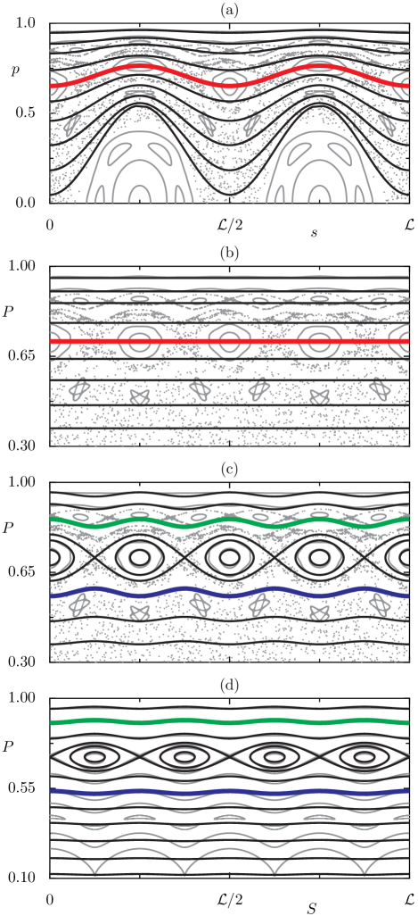
Figure 5: In (a) the phase space of the mixed system (gray dots and lines) is superimposed by the adiabatically invariant curves in black in Birkhoff coordinates. The thick red line corresponds to the adiabatically invariant action $P_{a:b}$. In (b) the same orbits and adiabatically invariant curves are shown in adiabatic action–angle coordinates. The phase space of the pendulum Hamiltonian is shown by black lines in (c) on top of the actual ray dynamics depicted in gray. The same scenario for the near-integrable system is shown in (d). In (c) and (d) an example of the torus $\tilde{P}_{m,l}$ (thick green line) and its symmetric counterpart $\tilde{P}_{\mathrm{rat}}$ (thick blue line) is shown.

III.2 Pendulum Hamiltonian

We continue with the construction of a pendulum Hamiltonian using the adiabatic action–angle coordinates introduced above. Such a Hamiltonian is known to describe the dynamics in the vicinity of a nonlinear resonance and to capture the essential features of resonance–assisted tunneling BroSchUll2002 . In the case of optical microcavities or billiards the Hamiltonian is given by Ozo1984 ; BroSchUll2002

$$H_{a:b}(S,P)=H_{0}(P)+2V_{a:b}\cos\left(\frac{2\pi}{\mathcal{L}}aS+\phi_{a:b}\right),$$ (17)

where $H_{0}(P)$ as well as the parameters $V_{a:b}$, and $\phi_{a:b}$ have to be determined by the dynamics of the original system.

In particular $H_{0}(P)$ encodes the frequencies $\omega(P)$ of motion along adiabatically invariant curves given by $P$. Neglecting the effects of the boundary deformation these frequencies are given by the frequencies of a circular cavity,

$$\omega(P)=\frac{\mathcal{L}}{\pi}\arccos(P).$$ (18)

A more rigorous argument leading to this equation can be made using averaging DulMei2012 for the effective map derived in Refs. RobBer1985 ; Noe1997 . In particular Eq. (18) guarantees the correct limit of whispering-gallery trajectories almost tangential to the boundary, i.e., $P=1$ corresponds to a line of fixed points as $\omega(1)=0$. On the other hand, as $\omega(0)=\mathcal{L}/2$, for the trajectory bouncing along the symmetry line of the billiard the arc-length coordinate $s$ advances by $\mathcal{L}/2$ between successive bounces. In between these extreme cases Eq. (18) follows the frequencies of the circular cavity up to rescaling by $\mathcal{L}/(2\pi R)$.

Given the frequency relation Eq. (18), an $a:b$ resonance occurs for $\omega_{a:b}=b\mathcal{L}/a$, i.e., for

$$P_{a:b}=\cos\left(\pi\frac{b}{a}\right).$$ (19)

This momentum $P_{a:b}$ corresponds to the adiabatically invariant curve which interpolates through the nonlinear resonance, i.e., on which the periodic orbits are located. For the relevant $a:b=4:1$ resonance the adiabatic curve corresponding to $P_{a:b}$ is shown as thick red line in Fig. 5(a) and (b).

In order to obtain the same frequencies as Eq. (18) relative to the resonant frequency we require $H_{0}^{\prime}(P)=\omega(P)-\omega_{a:b}$, which yields KulWie2016b

$$H_{0}(P)= \frac{\mathcal{L}}{\pi}\left(P\arccos(P)-\sqrt{1-P^{2}}+\sqrt{1-P_{a:b}^{2}}\right)$$

$$-\omega_{a:b}P.$$ (20)

The quadratic expansion of Eq. (20) around $P_{a:b}$ then leads to

$$H_{0}(P)=\frac{1}{2M_{a:b}}\left(P-P_{a:b}\right)^{2}$$ (21)

with

$$M_{a:b}=-\left(\frac{2\pi}{\mathcal{L}}\right)\frac{1}{2}\sqrt{1-P_{a:b}^{2}}.$$ (22)

Having fixed $M_{a:b}$ the parameter $V_{a:b}$ controls the width of the nonlinear resonance in phase space. For near-integrabe systems it is related to the area $\mathcal{A}_{a:b}$ enclosed by the separatrix of the unstable periodic points by EltSch2005

$$V_{a:b}=\left(\frac{2\pi}{\mathcal{L}}\right)^{2}\frac{\mathcal{A}_{a:b}^{2}}{512M_{a:b}}.$$ (23)

Further away from integrability, e.g. for the considered mixed system, this naturally generalizes to the area enclosed by the invariant manifolds of the unstable periodic points up to their first heteroclinic intersection. In contrast, for the near-integrable case $V_{a:b}$ is determined by the linearized dynamics around the stable periodic orbit in terms of its monodromy matrix $\mathcal{M}_{a:b}$, which is known analytically for billiard systems DulRicWit1996 . This yields

$$V_{a:b}=\left(\frac{\mathcal{L}}{2\pi}\right)^{2}\frac{M_{a:b}}{2a^{4}}\left[\arccos\left(\frac{\mathrm{Tr}\mathcal{M}_{a:b}}{2}\right)\right]^{2}$$ (24)

and is used for the near-integrable system investigated in this paper.

Finally, $\phi_{a:b}$ is fixed by matching the $S$-coordinate of the equilibria of the resonance in the Hamiltonian (17) with the periodic orbits of equal stability. The phase space of the resulting Hamiltonian for the mixed system and for the near-integrable system is shown in Fig. 5(c) and (d), respectively. Note, that in the near-integrable system good agreement between ray dynamics and pendulum Hamiltonian is already achieved, if all $\epsilon$ dependent corrections are neglected. However, we keep this corrections to study both the near-integrable and mixed system within the same framework.

III.3 EBK Quantization of Adiabatic Actions

As both the perturbative and the semiclassical description of resonance–assisted tunneling crucially depend on the pendulum Hamiltonian (17) defined on the boundary a connection between actual modes of the cavity and adiabatic invariants has to be established. In integrable systems this correspondence is given by means of EBK quantization of invariant tori of the full ray dynamics. In systems with two degrees of freedom the existence of such invariant tori implies the existence of a second conserved quantity besides energy. For the integrable elliptic cavity, which includes circular cavities as special case, this quantity is given by the adiabatic invariant $P$, i.e., $P$ is an actual invariant of the dynamics for all times. In contrast, for generic systems $P$ changes adiabatically. However, if this change is slow enough, the corresponding adiabatically invariant, two-dimensional tori may still be used for EBK quantization. However, good agreement with numerically determined wave numbers can only be expected, if the actual ray dynamics follows the adiabatic invariant curves for a sufficiently long time. This assumption is expected to be fulfilled when these curves are located in the regular part of phase space. In particular this is the case for whispering-gallery trajectories.

Following Refs. KelRub1960 ; NoeSto1997 ; Noe1997 the real part of the wave number associated with a quantizing, adiabatic invariant $P_{m,l}$ corresponding to a whispering–gallery mode with angular mode number $m$ and radial mode number $l$ is given by

$$\mathrm{Re}\,k_{m,l}=\frac{2\pi m}{n}\left(\int_{0}^{\mathcal{L}}p\left(s,P_{m,l}\right)\mathrm{d}s\right)^{-1}.$$ (25)

Here, the adiabatic invariant $P_{m,l}$ is required to fulfill the quantization condition Noe1997

$$m\left(L(0,s^{*})-\int_{0}^{s^{*}}p\left(s,P_{m,l}\right)\mathrm{d}s\right)$$

$$=\left(l+\alpha\right)\int_{0}^{\mathcal{L}}p\left(s,P_{m,l}\right)\mathrm{d}s,$$ (26)

where, $s^{*}$ denotes the arc–length coordinate of the first collision of a ray started with initial conditions $(0,p(0,P_{m,l}))$ on the boundary and $L(0,s^{*})$ denotes the geometric length of the ray segment in between the boundary points labeled by $s=0$ and $s=s^{*}$, respectively. The parameter $\alpha$ represents the phase shift that an incoming wave undergoes when it is reflected at the cavity boundary. Thus $\alpha$ takes the openness of the system and the corresponding boundary conditions into account. As there is no analytical result for $\alpha$ in the case of open cavities we fix its value at zero deformation where the wave numbers $k_{m,l}$ are known. Specifically, in the circular case Eq. (25) reduces to $p(s,P_{m,l})=P_{m,l}=m/(n\mathrm{Re\,}k_{m,l})$, which allows to fix $\alpha$ in Eq. (26). We further assume, that $\alpha$ remains constant under deformation of the boundary. This allows us to solve Eq. (26) numerically for $P_{m,l}$. For this purpose we use the exact expression (11) for $p(s,P_{m,l})$. Note, that Eq. (26) does not necessarily permit a solution for arbitrary $m$ and $l$. For instance in case of the mixed system studied in this paper we obtain $2l+1<m$ as a necessary condition for the existence of solutions.

The accuracy of this approach has been demonstrated in Ref. NoeSto1997 . When applied to the near-integrable and the mixed system the quantization scheme presented above yields good agreement with numerically computed wave numbers, as Fig. 6 shows. There, the normalized error

$$\Delta\mathrm{Re}\,k_{m,l}=\frac{|\mathrm{Re}\,k_{m,l}^{\mathrm{(EBK)}}-\mathrm{Re}\,k_{m,l}^{\mathrm{(BEM)}}|}{\mathrm{Re}\,k_{m,l}^{\mathrm{(BEM)}}}$$ (27)

between numerical (BEM) and semiclassical (EBK) obtained wave numbers is depicted as a function of the real part of the wave number. For both near-integrable system and mixed system, represented by the orange triangles and blue diamonds, respectively, the error becomes smaller with increasing real part of the wave number. In both cases larger deviations occur around the wave number with $m=23$, where the peak in the negative imaginary parts was observed. This can be traced back to the fact that the EBK quantization scheme neglects the coupling of modes associated with different quantizing adiabatic invariants while such mode coupling may cause a shift in the real part of the wave number. Overall, the relative error made by EBK quantization is slightly smaller in the near-integrable system.

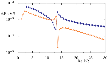
Figure 6: Relative errors of EBK wave numbers given by Eq. (27) for the near-integrable system (orange triangles) and for the mixed system (blue diamonds). The lines connecting the symbols are a guide to the eye.

III.4 Ray-Based Decay

While EBK quantization yields accurate real parts of the wave numbers, a ray-based quantitative description of their imaginary parts is available only for fully chaotic systems or the special case of the integrable circular cavity. However, in the following we present a ray-based model of decay rates, which yields good agreement with the numerically obtained imaginary parts of wave numbers.

To this end, we assign an effective reflectivity $R(P)$ for a light ray moving on an adiabatically invariant curve given by $P$. This is accomplished by averaging the reflectivity $R(p)$ of a circular cavity obtained in Ref. HenSch2002 along the adiabatically invariant curve defined by $P$ and Eq. (12). That is, we set

$$R(P)=\frac{1}{\mathcal{L}}\int_{0}^{\mathcal{L}}R(p(s,P))\frac{\partial S(s,P)}{\partial s}\mathrm{d}s$$ (28)

where a uniform density along the adiabatic curve in the adiabatic action–angle coordinates is assumed. The corresponding density $\partial S/\partial s$ in Birkhoff coordinates is obtained by differentiating Eq. (16) with respect to the arc-length coordinate. Equating the exponential decay in the wave and in the ray picture gives the decay rate HenSch2002

$$\Gamma=-2c\frac{\ln(R(P))}{4nR\sqrt{1-P^{2}}}$$ (29)

of a mode associated with $P$. Note that $P$ is not required to fulfill a quantization condition. Thus it is applicable for arbitrary $P$. In contrast, for quantizing $P=P_{m,l}$ we have

$$\mathrm{Im}\,k_{m,l}=-\frac{\Gamma_{m,l}}{2c}.$$ (30)

Strictly speaking this is only true for integrable systems, where the actual modes are associated with a single classical torus defined by $P_{m,l}$. We call $\Gamma_{m,l}$ the direct decay rate of this mode. For nonintegrable systems dynamical tunneling between quantizing adiabatically invariant tori will cause the decay rates and therefore also the imaginary parts of wave numbers to deviate from the direct decay given by Eq. (29).

III.5 Perturbation Theory of Resonance–Assisted Tunneling

While the ray-based model of decay describes the direct decay of an optical mode associated with the quantizing adiabatic invariant, resonance–assisted tunneling causes couplings to faster decaying modes. As these couplings are small, the real part of the wave numbers is expected to be not influenced by resonance–assisted tunneling, while the overall decay will increase. This enhancement is well described by quantum perturbation theory within the Hamiltonian (17). Based on this, we construct a perturbative expansion of the imaginary parts of the wave numbers $k_{m,l}$ for whispering–gallery modes with $l=0$. For quantum perturbation theory an unperturbed basis in terms of optical modes and wave numbers is required. As mentioned above, this is accomplished either by the circular cavity, which approximates the near-integrable system and the elliptic cavity approximating the mixed system, respectively. This allows for a perturbative treatment of resonance–assisted tunneling in both systems. Moreover, we will demonstrate that using the EBK quantization scheme and the ray-based model for the imaginary parts of wave numbers an actual approximating cavity is not necessary. More specifically, we construct the perturbative expansion solely from the EBK wave numbers, quantizing adiabatic invariants and the decay rates introduced in Sec. III.4.

In order to obtain a perturbative description we follow Refs. LoeBaeKetSch2010 ; SchMouUll2011 and apply the perturbation theory of resonance–assisted tunneling in quantum systems to optical microcavities. To this end let us denote the wave numbers of the approximating cavity by $\tilde{k}$ and expand the imaginary part of $k_{m,l}$ as LoeBaeKetSch2010 ; KulWie2016b

$$\mathrm{Im}\,k_{m,l}=\mathcal{N}^{-2}\sum_{v\geq 0}|c_{v}|^{2}\mathrm{Im}\tilde{k}_{m-va,l+vb}.$$ (31)

Here, $\mathcal{N}^{2}=\sum_{v\geq 0}|c_{v}|^{2}$ accounts for proper normalization and the sum is restricted by the requirement that all angular mode numbers $m-va$ have to be non-negative. Further note, that only wave numbers of modes within the same symmetry class contribute to the sum. The coefficients $c_{v}$ follow from the perturbative scheme developed in Ref. Loe1951 applied to the pendulum Hamiltonian (17) and adapted to optical systems LoeBaeKetSch2010 ; YiKulKimWie2017 . They are determined by the wave numbers of the approximating cavity and the corresponding quantizing adiabatic invariants. In order to compute the coefficients $c_{v}$ we make the following observations. Given an approximating cavity its adiabatically invariant curves, Eq. (11), should coincide with the adiabatically invariant curves of the original system. Therefore, by means of EBK quantization, the quantizing adiabatic invariants $P_{m-va,l+vb}$ coincide as well, if we further assume the length $L(0,s^{*})$ of the ray segment appearing in Eq. (26) to be approximately the same. Additionally this implies that also the real parts of the wave numbers in both systems agree, i.e., $\mathrm{Re\,}\tilde{k}_{m-va,l+vb}=\mathrm{Re\,}k_{m-va,l+vb}$. The coefficients $c_{v}$ can be computed by assigning an energy

$$E_{m-va,l+vb}=H_{0}(P_{m-va,l+vb}-\Delta p_{\mathrm{POS}}(k_{m-va,l+vb}))$$ (32)

in the Hamiltonian $H_{0}(P)$ given by Eq. (20) to each of the quantizing adiabatic invariants. Note, that here we take the periodic-orbit shift into account, which we assume to be the same in both coordinate systems as they are transformed into each other by a near identity transformation. This adjusts the effective position of the nonlinear resonance at $P_{a:b}+\Delta p_{\mathrm{POS}}(k_{m-va,l+vb})$ relative to $P_{m-va,l+vb}$. However, shifting the quantizing adiabatic invariants rather than $P_{a:b}$ allows to use the same Hamiltonian for all wave numbers. The coefficients in the perturbative expansion (31) then can be written as YiKulKimWie2017

$$c_{v}=\prod_{u\leq v}\frac{V_{a:b}(\mathrm{Re}\,k_{m,l})^{2}\text{e}^{\mathrm{i}\phi_{a:b}}}{E_{m,l}(\mathrm{Re}\,k_{m,l})^{2}-E_{m-ua,l+ub}(\mathrm{Re}\,k_{m-ua,l+ub})^{2}},$$ (33)

where in the product $u$ is restricted to those values for which the quantization condition Eq. (26) permits a solution. As the nonlinear resonance only couples modes whose wave numbers are similar, i.e., $\mathrm{Re}\,k_{m,l}\approx\mathrm{Re}\,k_{m-va,l+vb}$, the wave numbers in Eq. (35) cancel (up to small corrections) and $\Delta p_{\mathrm{POS}}(k)$ can be assumed to be constant for fixed $\mathrm{Re}\,k_{m,l}$. This additional approximation does not alter the end result significantly and thus we use

$$E_{m-va,l+vb}=H_{0}(P_{m-va,l+vb}-\Delta P_{\mathrm{POS}}(k_{m,l}))$$ (34)

as well as KulWie2016b

$$c_{v}=\prod_{u\leq v}\frac{V_{a:b}\text{e}^{\mathrm{i}\phi_{a:b}}}{E_{m,l}-E_{m-ua,l+ub}}$$ (35)

in the following. Further note, that so far for the evaluation of Eq. (35) only properties of the original system are required. In particular, it is not required that an approximating cavity exists.

Using the coefficients Eq. (35) and the imaginary parts of wave numbers in the circular and elliptic cavity we find overall good qualitative agreement with numerical obtained mode numbers in the near-integrable and the mixed system. This is shown in Fig. 7(a) and (b) where the numerically obtained wave numbers (black stars) are compared with Eq. (31) (red crosses). For the near-integrable system the wave numbers of the circular cavity can be obtained analytically. For the mixed system the eccentricity of the elliptic cavity is chosen according to Eq. (5) and the wave numbers are computed numerically. Thus for the mixed system the method provides no numerical advantage compared to the direct numerical computation of wave numbers. However it demonstrates the validity of the approach. In both systems we truncate the perturbative expansion, Eq. (31), at $v\leq 5$. In the near-integrable system the exponential decay of the negative imaginary part of the wave numbers match with the numerically obtained wave numbers. In contrast, in the mixed system the overall exponential decay matches up to the second peak only, but is slower than in the numerical data for larger real parts. We assume this to be caused by the Goos–Hänchen shift rendering the modified ray-dynamics of the elliptic cavity nonintegrable and the corresponding enhancement of the decay of its optical modes, which are used as an unperturbed basis. In both systems the first numerically obtained peak is described well. The subsequent peaks are predicted systematically for slightly smaller real parts of the wave numbers compared to the numerical data. The strong enhancement of the negative imaginary part of the wave number can be traced back to the coefficients Eq. (35) which diverge whenever a quantizing adiabatic invariant $P_{m-va,l+vb}$ is energetically degenerate with $P_{m,l}$ with respect to $H_{0}$ when the periodic-orbit shift is taken into account. Within the quadratic approximation of $H_{0}$ by Eq. (21) this corresponds to $P_{m+va,l-vb}$ and $P_{m,l}$ being located symmetrically around $P_{a:b}+\Delta p_{\mathrm{POS}}(k_{m,l})$. Deviations of the actual frequencies of motion along adiabatically invariant curves from those predicted by $H_{0}$ may shift the wave numbers for which this degeneracy occurs in the perturbative description. Further, this degeneracy may be spoiled by deviations of the periodic orbit shift from Eq. (6). In the mixed system the perturbative description fails when $\mathrm{Re}\,k_{m,l}R>25$ as it does not include additional resonances which may cause the formation of the observed plateau.

While the perturbative expansion gives rise to qualitatively, and for the near-integrable system also quantitatively, good agreement with numerical data, Eq. (31) still requires the knowledge of the imaginary parts of the wave numbers of the approximating integrable cavity. Replacing them by Eq. (30) and Eq. (29) evaluated at $P_{m-va,l+vb}$ allows for a prediction of wave numbers without making reference to an actual approximating cavity. The resulting wave numbers are shown as blue circles in Fig. 7. For the near-integrable system they perfectly match the prediction obtained above. In the case of the mixed system they underestimate the initial exponential decay by up to one order of magnitude. For larger real parts of the wave numbers they agree slightly better with the numerical data compared to the prediction using the wave numbers of the elliptic cavity up to the wave numbers where additional resonances may become important.

Using this ray-based model of decay allows for an application of perturbation theory when there is no actual approximating cavity. The remaining inaccuracy of the ray-based model can be associated with the approximate nature of both the adiabatically invariant curves and the associated effective reflectivity, Eq. (28). Moreover some of these adiabatically invariant curves are located partially in the chaotic region of the actual ray dynamics. Thus classical chaotic transport phenomena as well as chaos–assisted tunneling may influence the decay. These phenomena are not taken into account here.

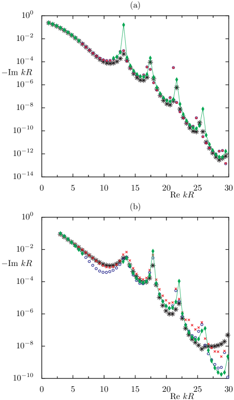
Figure 7: Wave numbers for the near-integrable systems are shown in (a) starting from $m=1$ and in (b) for mixed system starting from $m=4$. Numerical obtained wave numbers are depicted as black stars. The perturbative description using the imaginary parts of wave numbers in the circular and elliptic cavity is shown as red crosses while blue circles denote the perturbative description combined with the ray-based decay rates. The semiclassical description is represented by green diamonds. The lines connecting the data points are a guide to the eye.

III.6 Semiclassical description

While the perturbative description of resonance–assisted tunneling decomposes the imaginary part of the whispering gallery modes wave numbers into several contributions from different modes, in a semiclassical description there are only two contributions. In particular there is a direct contribution to the decay denoted as $\Gamma_{m,l}$ which resembles the decay of an optical mode associated with the quantizing adiabatic invariant $P_{m,l}$. Therefore, the direct contribution describes the decay of the mode that would be present even if the system was integrable, i.e., in the absence of nonlinear resonances and resonance–assisted tunneling. The contribution resulting from resonance–assisted tunneling is denoted by $\Gamma_{\mathrm{rat}}$ and is associated with an adiabatic invariant $P_{\mathrm{rat}}$ located symmetrically on the opposite side of the nonlinear resonance with respect to $P_{m,l}$. In general $P_{\mathrm{rat}}$ does not fulfill a quantization condition and thus is not associated with an actual mode of the system or of an approximating integrable cavity. To be more precise, an optical mode associated with $P_{m,l}$ obtained by EBK quantization will also localize on $P_{\mathrm{rat}}$. However, the amplitude on $P_{\mathrm{rat}}$ is suppressed by a factor $\mathcal{A}_{T}$ called the tunneling amplitude. Taken this into account the imaginary parts of the wave numbers can be decomposed as FriBaeKetMer2017

$$\mathrm{Im\,}k_{m,l}=-\frac{1}{2c}\Gamma_{m,l}-\frac{\mathcal{A}_{T}^{2}}{2c}\Gamma_{\mathrm{rat}}.$$ (36)

Here, $\Gamma_{m,l}$ is given by Eqs. (29) and (30) for $P=P_{m,l}$ and $\Gamma_{\mathrm{rat}}$ for $P=P_{\mathrm{rat}}$, respectively.

Thus it remains to compute $P_{\mathrm{rat}}$ and $\mathcal{A}_{T}$ in the following, which is done by means of WKB theory within the pendulum Hamiltonian (17) with quadratic $H_{0}(P)$, Eq. (21). Due to the periodic-orbit shift we consider $\tilde{P}_{m,l}=P_{m,l}-\Delta p_{\mathrm{POS}}(k_{m,l})$ for the semiclassic construction of $P_{\mathrm{rat}}$ and $\mathcal{A}_{T}$. The equally shifted $\tilde{P}_{\mathrm{rat}}=P_{\mathrm{rat}}-\Delta p_{\mathrm{POS}}(k_{m,l})$ is defined as the torus on the opposite side of the resonance with respect to $\tilde{P}_{m,l}$ but with the same energy $E_{m,l}=H_{0}(\tilde{P}_{m,l})$. It is given by $\tilde{P}_{\mathrm{rat}}=2P_{a:b}-\tilde{P}_{m,l}$. Both $\tilde{P}_{m,l}$ and $\tilde{P}_{\mathrm{rat}}$ are shown schematically in Fig. 5(c) and (d) for the mixed and the near integrable system as thick green and blue lines, respectively. In order to compute the tunneling amplitude we identify $1/(n\mathrm{Re}\,k_{m,l}R)$ as the semiclassical parameter which plays the role of the reduced Planck constant. Using this identification gives

$$\mathcal{A}_{T}=\left|2\sin\left(\frac{n}{2a}\mathrm{Re}\,k_{m,l}R\,\mathcal{A}_{\mathrm{rat}}\right)\right|^{-1}\exp{\left(-n\mathrm{Re}\,k_{m,l}R\,\sigma\right)}$$ (37)

for optical microcavities. Here,

$$\mathcal{A}_{\mathrm{rat}}=\mathcal{L}(P_{m,l}-P_{\mathrm{rat}})$$ (38)

is the phase-space area bounded by the adiabatic invariants $P_{m,l}$ and $P_{\mathrm{rat}}$ and $\sigma$ is determined by the imaginary action of complex classical paths which bridge the nonlinear resonance and connect $\tilde{P}_{m,l}$ with $\tilde{P}_{\mathrm{rat}}$. In particular, for the action of these complex paths we have

$$\sigma=\frac{\mathcal{A}_{\mathrm{rat}}}{2\pi a}\ln\left(\left|\frac{4E_{m,l}}{\text{e}^{2}V_{a:b}}\right|\right)$$ (39)

in analogy to Ref. BroSchUll2002 . In Fig. 7 we compare the wave numbers obtained by the semiclassical formula Eq. (36) with the numerical data. Note, that the semiclassical description is only valid if the quantizing adiabatic invariant is located outside of the $4:1$ resonance. Hence the initial exponential decay in both the near-integrable and the mixed system is due to the direct contribution in Eq. (36) as $\tilde{P}_{m,l}$ is located below the resonance while $\tilde{P}_{\mathrm{rat}}$ is located above. Therefore the direct contribution is dominant and the resonance–assisted contribution can safely be neglected. Similar to the perturbative description the initial decay is underestimated in the mixed system as Eq. (29) underestimates the actual decay within this regime. In between the initial decay and the first peak the quantizing adiabatic invariant $\tilde{P}_{m,l}$ is located inside the $4:1$ resonance and thus no meaningful semiclassical prediction based on Eq. (36) is possible. Once $\tilde{P}_{m,l}$ is located above the nonlinear resonance for larger real parts of wave numbers the semiclassical description is again applicable and leads to good agreement with the numerically obtained wave numbers. In particular, in this regime the resonance–assisted contribution dominates and the direct contribution can be neglected. In both systems the overall exponential decay is in good agreement with the numerical obtained wave numbers. Moreover, the position of the peaks is resolved correctly in both systems except for the peak around $\mathrm{Re}\,k_{m,l}R=25$ in the near-integrable system. The peaks occur whenever the prefactor that enters in Eq. (37) diverges, which occurs if $n\mathrm{Re}\,k_{m,l}R\,\mathcal{A}_{\mathrm{rat}}$ is an integer multiple of $2\pi a$. If this condition is fulfilled exactly, Eq. (37) is ill-defined, which causes the semiclassical prediction to overestimate the numerical obtained negative imaginary parts. At these wave numbers $P_{\mathrm{rat}}$ satisfies a quantization condition as well. That is $P_{\mathrm{rat}}=P_{m-va,l+vb}$ for some integer $v$. As, by definition, $P_{m,l}$ and $P_{\mathrm{rat}}$ are energetically degenerate this is the same condition obtained from the perturbative treatment of resonance–assisted tunneling. Again, for the mixed system, the semiclassical prediction does not capture the plateau formation for wave numbers $\mathrm{Re}\,k_{m,l}R>25$, which we expect to be due to additional resonances.

Although being at least equally accurate as the perturbative description the semiclassical picture is also subject to the same errors induced by the ray-based model of decay as discussed in the previous section.

IV summary and outlook

In this paper we demonstrate how resonance–assisted tunneling gives rise to enhanced decay of optical modes in deformed microdisks with near-integrable or mixed phase space. While the near-integrable case was treated before we extend the existing perturbative description to systems far from integrabillity and presented also a semiclassical description. We apply both the perturbative and the semiclassical description to systems with either near-integrable or mixed classical ray dynamics and find good agreement with numerically obtained data for whispering–gallery modes. In particular our description correctly captures the overall exponential decay of the imaginary parts of wave numbers towards larger wave numbers and predicts the wave numbers of modes with significantly enhanced decay. In the latter case the semiclassical description gives rise to better agreement with the numerical obtained positions of these peaks compared to perturbation theory. Moreover, we show that the theory of resonance–assisted tunneling predicts the enhancement of decay in cases where the second order perturbative expansion in the deformation parameter does not apply.

Our approach is based on the construction of adiabatically invariant action–angle coordinates and the approximation of the relevant nonlinear resonance by a suitable pendulum Hamiltonian. We further use EBK quantization of adiabatic invariants and a ray-based model for the decay of optical modes to compute wave numbers in the absence of dynamical tunneling. The obtained imaginary parts of the wave numbers can be interpreted as the direct decay of the associated modes. Subsequently, the pendulum Hamiltonian allows for the inclusion of resonance–assisted tunneling by either quantum perturbation theory or a semiclassical description. Both descriptions confirm that the underlying mechanism of enhancement coincides with what is known for two-dimensional quantum maps. That is, the enhancement is due to the coupling of optical modes associated with quantizing adiabatic invariants which are located symmetrical with respect to the relevant nonlinear resonance. This allows whispering gallery modes with slow decay to couple to faster decaying modes, which can be seen also in their Husimi representation. While the coupling between modes is well described within the pendulum Hamiltonian the main error of the presented approach is introduced by describing the direct decay based on a simple ray picture.

In the regime of large wave numbers we expect also smaller resonances to become important for tunneling as the numerical obtained wave numbers in the mixed system suggest. These multi-resonance effects could be incorporated in the perturbative description, as it was done for quantum maps. However, a semiclassical picture thereof does not exist so far.

Furthermore, an obvious generalization of the deformed microdisks are three-dimensional deformed spherical cavities, which are expected to exhibit resonance–assisted tunneling as well. As such cavities are frequently used in experiments an equally good description as in the two-dimensional case is of great interest. However, with more degrees of freedom resonances of higher rank may arise which give rise to a much more complex way of resonance–assisted coupling between optical modes. This was recently demonstrated for a normal–form Hamiltonian FirFriKetBae2019 . On an even more fundamental level the interplay of tunneling and classical transport mechanisms, e.g., the famous Arnold diffusion, could become important in three-dimensional cavities. This is, however, even an open problem for much simpler systems like four-dimensional symplectic maps.

- (1) K. Vahala (editor) Optical Microcavities, volume 5 of Advanced Series in Applied Physics, World Scientific, Singapore (2004).
- (2) H. Cao and J. Wiersig, Dielectric microcavities: Model systems for wave chaos and non-Hermitian physics, Rev. Mod. Phys. 87, 61 (2015).
- (3) M. R. Foreman, J. D. Swaim, and F. Vollmer, Whispering gallery mode sensors, Advances in Optics and Photonics 7, 168 (2015).
- (4) L. He, Ş. K. Özdemir, and L. Yang, Whispering gallery microcavity lasers, Laser Photonics Rev. 7, 60 (2013).
- (5) J. U. Nöckel, A. D. Stone, G. Chen, H. L. Grossman, and R. K. Chang, Directional emission from asymmetric resonant cavities, Optics Letters 21, 1609 (1996).
- (6) J. Wiersig and M. Hentschel, Combining directional light output and ultralow loss in deformed microdisks, Phys. Rev. Lett. 100, 033901 (2008).
- (7) V. F. Lazutkin, The existence of caustics for a billiard problem in a convex domain, Math. USSR Izv. 7, 185 (1973).
- (8) M. J. Davis and E. J. Heller, Quantum dynamical tunneling in bound states, J. Chem. Phys. 75, 246 (1981).
- (9) S. Keshavamurthy and P. Schlagheck, Dynamical Tunneling: Theory and Experiment, Taylor & Francis, Boca Raton (2011).
- (10) C. Dembowski, H.-D. Gräf, A. Heine, R. Hofferbert, H. Rehfeld, and A. Richter, First experimental evidence for chaos-assisted tunneling in a microwave annular billiard, Phys. Rev. Lett. 84, 867 (2000).
- (11) A. Bäcker, R. Ketzmerick, S. Löck, M. Robnik, G. Vidmar, R. Höhmann, U. Kuhl, and H.-J. Stöckmann, Dynamical tunneling in mushroom billiards, Phys. Rev. Lett. 100, 174103 (2008).
- (12) B. Dietz, T. Guhr, B. Gutkin, M. Miski-Oglu, and A. Richter, Spectral properties and dynamical tunneling in constant-width billiards, Phys. Rev. E 90, 022903 (2014).
- (13) S. Gehler, S. Löck, S. Shinohara, A. Bäcker, R. Ketzmerick, U. Kuhl, and H.-J. Stöckmann, Experimental observation of resonance-assisted tunneling, Phys. Rev. Lett. 115, 104101 (2015).
- (14) G. Hackenbroich and J. U. Nöckel, Dynamical tunneling in optical cavities, Europhys. Lett. 39, 371 (1997).
- (15) V. A. Podolskiy and E. E. Narimanov, Chaos-assisted tunneling in dielectric microcavities, Opt. Lett. 30, 474 (2005).
- (16) A. Bäcker, R. Ketzmerick, S. Löck, J. Wiersig, and M. Hentschel, Quality factors and dynamical tunneling in annular microcavities, Phys. Rev. A 79, 063804 (2009).
- (17) S. Shinohara, T. Harayama, T. Fukushima, M. Hentschel, T. Sasaki, and E. E. Narimanov, Chaos-assisted directional light emission from microcavity lasers, Phys. Rev. Lett. 104, 163902 (2010).
- (18) S. Shinohara, T. Harayama, T. Fukushima, M. Hentschel, S. Sunada, and E. E. Narimanov, Chaos-assisted emission from asymmetric resonant cavity microlasers, Phys. Rev. A 83, 053837 (2011).
- (19) J. Yang, S.-B. Lee, S. Moon, S.-Y. Lee, S. W. Kim, T. T. A. Dao, J.-H. Lee, and K. An, Pump-induced dynamical tunneling in a deformed microcavity laser, Phys. Rev. Lett. 104, 243601 (2010).
- (20) H. Kwak, Y. Shin, S. Moon, S.-B. Lee, J. Yang, and K. An, Nonlinear resonance-assisted tunneling induced by microcavity deformation, Sci. Rep. 5, 9010 (2015).
- (21) C.-H. Yi, H.-H. Yu, J.-W. Lee, and C.-M. Kim, Fermi resonance in optical microcavities, Phys. Rev. E 91, 042903 (2015).
- (22) C.-H. Yi, H.-H. Yu, and C.-M. Kim, Resonant torus-assisted tunneling, Phys. Rev. E 93, 012201 (2016).
- (23) J.-B. Shim, P. Schlagheck, M. Hentschel, and J. Wiersig, Nonlinear dynamical tunneling of optical whispering gallery modes in the presence of a Kerr nonlinearity, Phys. Rev. A 94, 053849 (2016).
- (24) J. Kullig and J. Wiersig, spoiling in deformed optical microdisks due to resonance-assisted tunneling, Phys. Rev. E 94, 022202 (2016).
- (25) C.-H. Yi, J. Kullig, C.-M. Kim, and J. Wiersig, Frequency splittings in deformed optical microdisk cavities, Phys. Rev. A 96, 023848 (2017).
- (26) O. Brodier, P. Schlagheck, and D. Ullmo, Resonance-assisted tunneling, Ann. Phys. (N.Y.) 300, 88 (2002).
- (27) O. Brodier, P. Schlagheck, and D. Ullmo, Resonance-assisted tunneling in near-integrable systems, Phys. Rev. Lett. 87, 064101 (2001).
- (28) C. Eltschka and P. Schlagheck, Resonance- and chaos-assisted tunneling in mixed regular-chaotic systems, Phys. Rev. Lett. 94, 014101 (2005).
- (29) S. Löck, A. Bäcker, R. Ketzmerick, and P. Schlagheck, Regular-to-chaotic tunneling rates: From the quantum to the semiclassical regime, Phys. Rev. Lett. 104, 114101 (2010).
- (30) P. Schlagheck, A. Mouchet, and D. Ullmo, Resonance-assisted tunneling in mixed regular-chaotic systems, in “Dynamical Tunneling: Theory and Experiment”, KesSch2011 , chapter 8, 177.
- (31) R. Dubertrand, E. Bogomolny, N. Djellali, M. Lebental, and C. Schmit, Circular dielectric cavity and its deformations, Phys. Rev. A 77, 013804 (2008).
- (32) M. Robnik and M. V. Berry, Classical billiards in magnetic fields, J. Phys. A 18, 1361 (1985).
- (33) J. B. Keller and S. I. Rubinow, Asymptotic solution of eigenvalue problems, Ann. Phys. (N.Y.) 9, 24 (1960), erratum, ibid, 10 (1960) 303–305.
- (34) J. U. Nöckel and A. D. Stone, Ray and wave chaos in asymmetric resonant optical cavities, Nature 385, 45 (1997).
- (35) J. U. Nöckel, Resonances in Nonintegrable Open Systems, Ph.D. thesis, Yale University (1997).
- (36) F. Goos and H. Hänchen, Ein neuer und fundamentaler Versuch zur Totalreflexion, Ann. Phys. 436, 333 (1947).
- (37) K. Artmann, Berechnung der Seitenversetzung des totalreflektierten Strahles, Ann. Phys. 437, 87 (1948).
- (38) J. Unterhinninghofen and J. Wiersig, Interplay of Goos-Hänchen shift and boundary curvature in deformed microdisks, Phys. Rev. E 82, 026202 (2010).
- (39) A. Bäcker, Numerical aspects of eigenvalues and eigenfunctions of chaotic quantum systems, in M. Degli Esposti and S. Graffi (editors) “The Mathematical Aspects of Quantum Maps”, volume 618 of Lect. Notes Phys., 91, Springer-Verlag, Berlin (2003).
- (40) J. Wiersig, Boundary element method for resonances in dielectric microcavities, J. Opt. A: Pure Appl. Opt. 5, 53 (2003).
- (41) R. Kress, Boundary integral equations in time-harmonic acoustic scattering, Mathl. Comput. Modelling 15, 229 (1991).
- (42) M. Hentschel, H. Schomerus, and R. Schubert, Husimi functions at dielectric interfaces: Inside-outside duality for optical systems and beyond, Europhys. Lett. 62, 636 (2003).
- (43) A. M. Ozorio de Almeida, Tunneling and the semiclassical spectrum for an isolated classical resonance, J. Phys. Chem. 88, 6139 (1984).
- (44) H. R. Dullin and J. D. Meiss, Resonances and twist in volume-preserving mappings, SIAM J. Appl. Dyn. Syst. 11, 319 (2012).
- (45) H. R. Dullin, P. H. Richter, and A. Wittek, A two‐parameter study of the extent of chaos in a billiard system, Chaos 6, 43 (1996).
- (46) M. Hentschel and H. Schomerus, Fresnel laws at curved dielectric interfaces of microresonators, Phys. Rev. E 65, 045603(R) (2002).
- (47) P.-O. Löwdin, A note on the quantum-mechanical perturbation theory, J. Chem. Phys. 19, 1396 (1951).
- (48) F. Fritzsch, A. Bäcker, R. Ketzmerick, and N. Mertig, Complex-path prediction of resonance-assisted tunneling in mixed systems, Phys. Rev. E 95, 020202(R) (2017).
- (49) M. Firmbach, F. Fritzsch, R. Ketzmerick, and A. Bäcker, Resonance-assisted tunneling in four-dimensional normal-form Hamiltonians, Phys. Rev. E 99, 042213 (2019).