Electron collimation at van der Waals domain walls in bilayer graphene

Abstract

We show that a domain wall separating single layer graphene (SLG) and AA-stacked bilayer graphene (AA-BLG) can be used to generate highly collimated electron beams which can be steered by a magnetic field. Two distinct configurations are studied, namely, locally delaminated AA-BLG and terminated AA-BLG whose terminal edge-type are assumed to be either zigzag or armchair. We investigate the electron scattering using semi-classical dynamics and verify the results independently with wave-packed dynamics simulations. We find that the proposed system supports two distinct types of collimated beams that correspond to the lower and upper cones in AA-BLG. Our computational results also reveal that collimation is robust against the number of layers connected to AA-BLG and terminal edges.

I Introduction

In the absence of scattering, the wave nature of electrons results in the analogy between optical and electronic transportCheianov2007 ; Banszerus2016 ; Wang2018a . This analogy has provided many novel phenomena in solid-state two-dimensional electron systems such as lensesSivan1990 , beam splittersOliver1999 , and wave guidesHartmann2010 ; Williams2011 . In conventional np junctions, optic-like manipulation of electron beams is hindered by the poor electron transmitters. However, in graphene Novoselov_2004 ; Geim_2007 electron transmission is enhanced due to Klein tunnelingBeenakker2008 ; Klein_1929 ; Stander2009 ; Katsnelson2006 ; Gutierrez2016 ; Abdullah2018a . Moreover, its energy spectrum resembles that of photons which allows experimentalists to use graphene as a test bed for optic-like electron behaviors. For example, two experiments were conducted recently where a negative refraction was observed for Dirac fermions in grapheneLee2015 and the angle-dependent transmission coefficient was simultaneously measuredChen2016 . The negative refraction index in graphene was predicted earlierCheianov2007 where it was found that electrons passing through np junction at specific energy converge on the other side at the focal point. This behavior is the analog of a Veselago lensVeselago1968 that was realized earlier in photonic crystalsParimi2004 ; Cubukcu2003 and metamaterialsSong2018 ; Houck2003 ; Grbic2004 . These findings led to profound theoretical investigations of electron focusing in SLGAidala2007 ; LaGasse2017 ; Zhang2018 as well as in AA-Sanderson_2013 and AB-BLGPeterfalvi2012 where a valley selective electronic Veselago lens was proposed.

Another analogue to light rays across an optical boundary is the collimation of electrons across np junction. This analog becomes perfect in the absence of scattering; however, the disorder-induced scattering has precluded the implementation of such an idea. Different proposals have been introduced to maintain collimation of an electron beam such as using graphene superlattices with periodicPark2008 or disorderedChoi2014 potentials. Another route was also established by introducing a mechanical deformation to form a parabolic pn junctionLiu2017a or carving pinhole slits in hexagonal Boron Nitride (hBN) encapsulated grapheneBarnard2017 as well as creating zigzag side contacts Bhandari2018 .

Motivated by the recent experiments where a point source of current in single layer graphene Handschin2015 ; Kinikar2017 and bilayerOverweg2017 were achieved, we propose a new system to obtain a highly collimated electron beam which can be used, for example, in Dirac fermion microscopeBoggild2017 . We consider a junction composed of single layer graphene and AA-BLG. Such system can exist in two configurations where delaminated bilayer graphene or single layer graphene are connected into AA-BLG as shown in Figs. 1(e) and (f), respectively. Recently, it was shown that such systems exhibit distinct electronic propertiesAbdullah2017 ; Abdullah2018 ; Abdullah2018b ; Abdullah_2016 ; Lane2018 ; Mirzakhani2016 . In the low-energy regime, the Fermi circle in delaminated region is much smaller than its counterpart in the AA-BLG. This results in a small refraction index forcing the transmitted electrons to nearly move in the same direction.

In this Article we calculate and compare the collimation of divergent electron beams using two distinct formalisms. In the first approach, we combine in a semi-classical (SC)Reijnders2013 ; Milovanovic2015 ; Peterfalvi2012 ; Reijnders2017 ; Milovanovic2014 way quantum mechanical calculation of the transmission probabilities at a domain wall with a wave propagation described as an optical analog. In the second approach we calculate the wave-packet dynamics (WD)Choi2014 ; Park2008 ; Maksimova2008 ; Chaves2010 ; Krueckl2009 of electrons incident on a domain wall to obtain the carriers trajectories. To control the direction of the collimated beam, we used a magnetic field to steer the electron beam. In the first configuration, we assume that a point source is located in the delaminated bilayer graphene and electrons are emitted and transmitting into AA-BLG. We find that electrons belonging to the lower and upper cones, within a specific energy range, are bent in diametrically opposite directions. This is a manifestation of the fact that the lower cone corresponds to electron-like particles while the upper cone acts as a dispersion of hole-like particles.

We also show the collimation in the second configuration where single layer graphene is connected to AA-BLG with zigzag or armchair edges as depicted in Fig. 1(f). Armchair and zigzag are the two types of edges which are most frequently considered in the study of graphene and BLG samples, although other types of terminations exist due to edge reconstruction. We found that the collimation is robust against the edge shape and the number of layers connected to AA-BLG and we found that the same collimation effects persist.

This paper is organized as follows. In Sec. II we describe the proposed system and present the model. Sec. III is devoted to numerical results and discussions of collimation and comparison of the two approaches SC and WD. Finally, we conclude by stressing our main findings in Sec. IV.

II Model

II.1 Atomic structures and boundary conditions

The crystalline structures of single layer graphene and AA-BLG are illustrated in Figs. 1(a, b) with the corresponding energy spectrum in Figs. 1(c, d), respectively. SLG has a hexagonal crystal structure comprising two atoms $A$ and $B$ in its unit cell with interatomic distance $a=0.142$ nm and intra-layer coupling $\gamma_{0}=3$ eVZhang_2011 . In the AA-BLG the two SLG are placed exactly on top of each other with a direct inter-layer coupling $\gamma_{1}\approx 0.2\$eV Li2009 ; Xu_2010 ; Lobato_2011 , see dashed-green vertical lines in Fig. 1(d). Pristine AA-BLG has a linear energy spectrum that consists of two Dirac cones (lower and upper cones) shifted by $2\gamma_{1}$, see blue and red cones in Fig. 1(d). These two cones are completely decoupledSanderson_2013 such that electron- and hole-like carriers are associated with each cone.

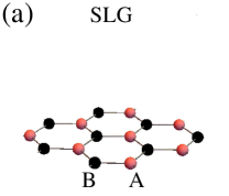
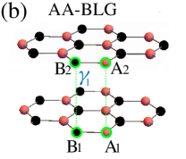
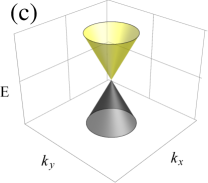
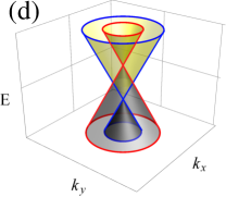
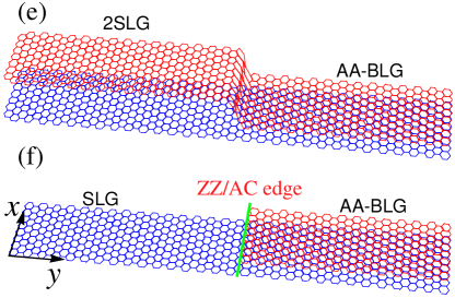
Figure 1: (Color online) Lattice structure with their corresponding energy spectrum of (a) SLG, (b) AA-BLG. (c) and (d) Yellow and black bands correspond to electrons and holes in SLG while in AA-BLG they represent electron- and hole-like states. Red and blue bands represent the upper and lower Dirac cones in AA-BLG. (e) Schematic illustration of delaminated BLG connected to AA-BLG, and (f) SLG attached to AA-BLG whose terminated edge of the top layer are either zigzag or armchair.

The general form of the Hamiltonian within the continuum approximation describing the charge carriers near the K-point in reciprocal space is a $4\times 4$ matrix in the basis $\mathbf{\Psi}=(\Psi_{A1},\Psi_{B1},\Psi_{A2},\Psi_{B2})^{T},$ whose elements refer to the sublattices in each layer. Transport in both connected and disconnected regions can be described by the following Hamiltonian

$$\mathcal{H}=\left(\begin{array}[]{cccc}v_{0}&v_{F}\hat{\pi}_{+}&\tau\gamma_{1}&0\\ v_{F}\hat{\pi}_{-}&v_{0}&0&\tau\gamma_{1}\\ \tau\gamma_{1}&0&v_{0}&v_{F}\hat{\pi}_{+}\\ 0&\tau\gamma_{1}&v_{F}\hat{\pi}_{-}&v_{0}\\ \end{array}\right),$$ (1)

where $v_{F}\approx 10^{6}$ m/s is the Fermi velocityCastro_Neto_2009 of charge carriers in each graphene layer, $\hat{\pi}_{\pm}=p_{x}\pm ip_{y}$ denotes the momentum, $v_{0}$ is the strength of a local electrostatic potential. The coupling between the two graphene layers is controlled by the parameter $\tau$ through which we can “switch on" or “switch off" the inter-layer hopping between the sublattices. For $\tau=0$, the two layers are decoupled and the Hamiltonian reduces to two independent SLG sheets while for AA-stacking we take $\tau=1$. The domain wall under consideration in this Article is, therefore, described by a local change in $\tau$ from zero to one.

Finally, notice that for the second configuration of this study, where transport from a single layer into an AA-bilayer system is considered, the Hamiltonian in Eq. (1) does not suffice. Rather, one needs to resort to the $2\times 2$ upper-left block that describes transport in a single layer of graphene. The effect of the atomic structure on the electronic transport is in this case determined through the boundary conditions (BCs).

The collimation occurs at the boundary between two stacking types. The terminated edge of AA-BLG can cross the lattice at any angle. At specific angles there are in general two distinct edges, namely, zigzag and armchair edgesNakanishi_2010 . Imposing zigzag boundary can be established through two different ways, namely, ZZ1 and ZZ2 where the sublattices $\phi_{B2}$ and $\phi_{A2}$ are set to be zero at the edge, respectivelyNakanishi_2010 . Note that the two types of the zigzag edges are equivalent in AA-BLG such that $T_{ZZ1}(\phi)=T_{ZZ2}(-\phi)$, where $T$ is the transmission probability, while this is not the case for AB-BLG. This can be attributed to the symmetric and asymmetric inter-layer coupling in, respectively, AA-BLG and AB-BLG. For the armchair edge, the single valley approximation is not valid anymore and thus the BCs are inter-valley mixed such thatNakanishi_2010

$$\phi_{A2}^{K}-\phi_{A2}^{K^{{}^{\prime}}}=0,\text{ and }\phi_{B2}^{K}+\phi_{B2}^{K^{{}^{\prime}}}=0.$$ (2)

II.2 Semi-classical dynamics

To describe electron dynamics semi-classically one proceeds in two steps. We first use the quantum mechanical formalism to evaluate transmission and reflection probabilitiesAbdullah2017 ; Barbier01_2010 ; Van_Duppen01_2013 ; Abdullah_2017 , and secondly determine the electron trajectories using the classical approach. Since the system is invariant along the $x-$direction, the solution of the Schrödinger equation $\rm H{\bf{\Psi}}=E\bf{\Psi}$ can be written in a matrix form as

$${\bf{\Psi}}(x,y)=M(y)Ce^{ik_{x}x},$$ (3)

where the $4\times 4$ matrix $M(y)$ represents the plane wave solutions, and the four-component vector $C$ contains the different coefficients expressing the relative weights of the different traveling modes, which have to be set according to the propagating region. After obtaining the desired solutions on both sides of the domain wall, we then implement the transfer matrix together with appropriate boundary conditions to obtain the transmission and reflection probabilities.

To calculate the electron trajectories, we assume a divergent beam starting from a focal point with a wave propagation given by the wave vector $\boldsymbol{k}$. The difference in wave vector between the connected and delaminated regions is determined by the relative refractive indexPereira2010 ; Cheianov2007 ; Milovanovic2015 ; Masirz2010 ; Barbier2010 ; Lee2015

$$n=\frac{\sin\theta}{\sin\phi}=\frac{k^{\prime}_{y}}{k_{y}},$$ (4)

where $\phi$ and $\theta$ are the incident and transmitted angles, respectively, while $k^{\prime}_{y}$ and $k_{y}$ are the wave vectors of the incident and transmitted electrons, respectively. For 2SLG-AA junction these wave vectors are given by

$$k^{\prime}_{y}=\frac{E}{v_{F}\hbar},\ \ k_{y}^{\pm}=\frac{1}{v_{F}\hbar}(\epsilon\pm\gamma_{1}),$$ (5)

where $\epsilon=E-v_{0}$ and $E$ is the Fermi energy. Using the above equations one can obtain the classical trajectoriesReijnders2017 ; Park2011 ; Phong2016 ; Milovanovic2014 ; Peterfalvi2012 . In Fig. 2(a), we show the system geometry (top panel) and the transmitted angle (bottom panel), according to Eq. (4), associated with the lower and upper cones. To achieve perfect collimation, the transmission angle must be zero which corresponds to zero refraction index. The refraction index of electrons incident from SLG and transmitted into gated AA-BLG is shown in Fig. 2(c) as a function of the electrostatic gate $v_{0}$. It is clear that the refraction index is almost zero in pristine AA-BLG, i.e. $v_{0}=0$. Henceforth, the gate will be considered zero and the calculations will be based only on pristine AA-BLG. A schematic presentation of the classical trajectories of carriers with different refraction indices is shown in Fig. 2(b) and our interest is when $n=0$ where carriers move in one dimension.

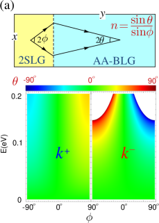
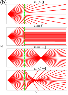
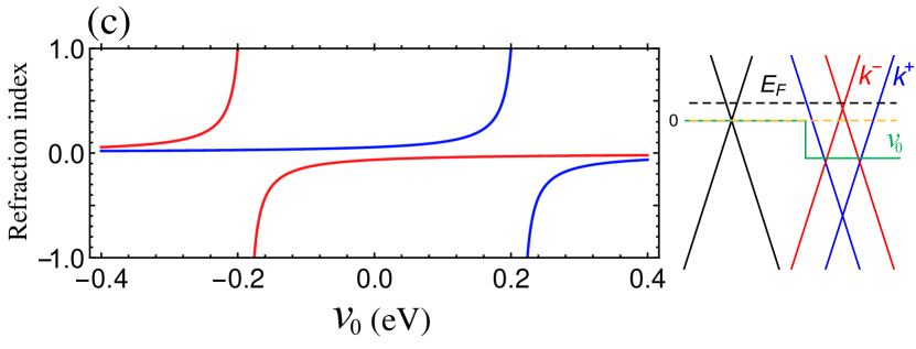
Figure 2: (Color online) (a) Top panel illustrates the 2SLG-BLG junction with incident and transmitted electron beams in the $x-y$ plane, while the bottom panel shows the transmitted angle $\theta$ as a function of the Fermi energy and the incident angle $\phi$ for SLG-AA junctions with $v_{0}=0.1$ eV. (b) Classical trajectories of an electronic beam impinging on media with different refraction indices. (c) Refraction index with the corresponding band diagram for SLG-AA as a function of the electrostatic potential strength $v_{0}$ where the Fermi energy of the incident particles is $E=12$ meV. Blue and red curves correspond to the different modes in AA-BLG region.

In the presence of a perpendicular magnetic field $\boldsymbol{B}$, the motion of the charge carriers follows a curved trajectory with curvature radius $r^{c}$. In the ballistic transport regime, where the Fermi wavelength is much smaller than the geometric size of the system, the charge carriers can be treated as classical point-like particles. Thus, we can calculate the cyclotron radius $r^{c}$ following Lorentz law described by

$$m\boldsymbol{a}=-e\boldsymbol{v}\times\boldsymbol{B},$$ (6)

where $e$ is the elementary charge, $\boldsymbol{a}$ and $\boldsymbol{v}$ are the acceleration and speed of electron, respectively. Note that the electron’s speed $\left|\boldsymbol{v}\right|$ will be assumed here to be the Fermi speed $v_{F}$. The effective mass $m$ of a particle in an isotropic energy spectrum readsAriel2013 ; Ashcroft1976 ; Zou2011

$$m=\frac{\hbar^{2}}{2\pi}\frac{dA(E)}{dE},$$ (7)

where $A(E)$ indicates the area in $k-$ space enclosed by a constant energy contour $E$. This area is circular in single layer graphene and AA-BLG. Note that depending on the energy curvature whether it is convex or concave, carriers can have a negative effective mass which is attributed to hole-like particles. Consequently, in the presence a magnetic field carriers with opposite sign of the effective mass will be deflected in opposite direction, as we will explore in the next sections. From Eqs. (6) and (7) we can obtain the cyclotron radius for AA-BLG and SLG as follows:

$$r_{\xi}^{c}(E)=\frac{\left|E\pm\xi\ \gamma_{1}\right|}{ev_{F}\left|B\right|},$$ (8)

where $E$ is the Fermi energy and $\xi=0$ or $1$ for SLG and AA-BLG, respectively. Finally, the equations of motion in the $x-y$ plane can be written as

$$x(t)=x_{\xi}-r_{\xi}^{c}\cos\left(\frac{v_{F}}{r_{\xi}^{c}}t+\Phi_{\xi}\right)+r_{\xi}^{c}\cos\left(\Phi_{\xi}\right),$$ (9a)

$$y(t)=y_{\xi}+r_{\xi}^{c}\sin\left(\frac{v_{F}}{r_{\xi}^{c}}t+\Phi_{\xi}\right)-r_{\xi}^{c}\sin\left(\Phi_{\xi}\right),$$ (9b)

where the point source of current is at $(x_{0},y_{0})$ in the SLG region while $(x_{1},y_{1})$ indicates the point where the electron hits the domain wall. $\Phi_{0(1)}$ represents the incidence (transmission) angle $\phi(\theta)$ described in the top panel of Fig. 2(a). Note that for $\xi=0$, $t$ is the time interval for the electron calculated once it is emitted from the current source while for $\xi=1$ it is the period of time calculated once the electron enters the AA-BLG region. Using the above equations we can trace the trajectories of the charge carriers in a magnetic field. In Fig. 3, we show the cyclotron radii for SLG and AA-BLG as a function of the magnetic field at different Fermi energies. At low energy, we see that the SLG cyclotron radius is sensitive to the magnetic field while in AA-BLG the cyclotron radii of the lower and upper cones (blue and red curves, respectively) are almost the same, see Fig. 3(a). Note that as a result of the spectrum resemblance of SLG and AA-BLG, we have $r^{c}_{AA}(E)=r^{c}_{SL}(E\pm\gamma_{1})$ which can be inferred from Figs. 3(b, c).

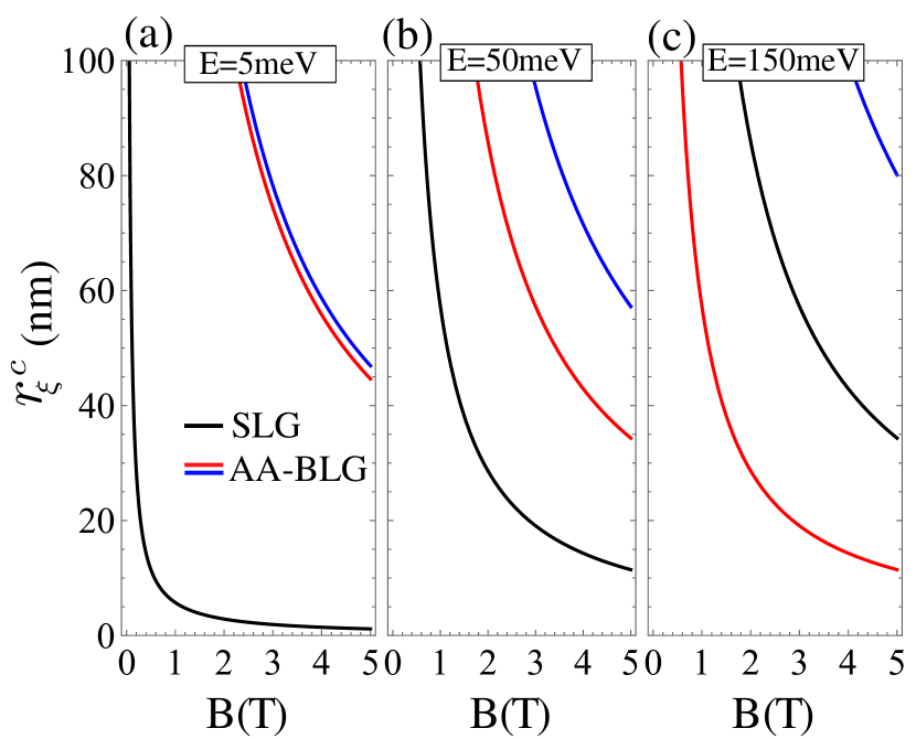
Figure 3: (Color online) Cyclotron radius in pristine (black curves) SLG and in AA-BLG for different Fermi energy. The red and blue curves correspond to the upper and lower cones in AA-BLG, respectively.

II.3 Wave packet dynamics

To calculate the quantum electronic trajectories using a wave packet, we apply the nearest-neighbor tight-binding model Hamiltonian for the description of electrons in a BLG system associated with the split-operator techniqueBatista2018 ; Costa2017 ; Chaves2015a ; Cavalcante2016 ; Costa2012 ; da_Costa_2015 ; Chaves2010 ; Chaves2009 ; Degani2010 ; Chaves2015 ; Rakhimov2011 . We have added to this technique the van der Waals domain walls as a local variation in the inter-layer coupling parameter as described by the parameter $\tau$ in Eq. (1). Following the numerical procedure developed in details by da Costa et al. in Ref. [da_Costa_2015, ], that is based on the split-operator technique, we calculate the time-evolution of the wave packet for two different set-ups composed of two disconnected SLG bounded with a AA-stacked BLG and one SLG bounded with a AA-stacked BLG.

Among the many different techniques to treat the formal solution of the time-evolution problem, such as Green’s functions techniquesKramer2011 , here we decided to choose the split-operator technique, since using this approach, one has the possibility of observing the transmitted and reflected trajectories of the total wave packet describing the electron propagating through the system, as well as the separated trajectories in each layer and also the scattered trajectories projected on the different Dirac cones. Moreover, this approach has the advantage of being faster and easier than e.g. Green’s functions techniques and, is pedagogical and physically a transparent approach for the understanding of transport properties in quantum systems, like the ones studied here.

The wave packet propagates in a system obeying the time-dependent Schrödinger equation $i\hbar\partial\mathbf{\Psi}(\boldsymbol{r},t)=H\mathbf{\Psi}(\boldsymbol{r},t)$, where the Hamiltonian $H$ is the nearest-neighbor tight-binding Hamiltonian given by

$$H_{TB}=\sum_{i\neq j}(\gamma_{ij}c_{i}^{\dagger}c_{j}+h.c)+\sum_{i}(\epsilon_{i}+V_{i})c^{\dagger}_{i}c_{i},$$ (10)

where $c_{i}$($c_{i}^{\dagger}$) annihilates (creates) an electron in site $i$ with on-site energy $\epsilon_{i}$, $\gamma_{ij}$ is the nearest-hopping energy between adjacent atoms $i$ and $j$, and $V_{i}$ is the on-site potential. The effect of an external magnetic field can be introduced in the tight-binding model by including a phase in the interlayer hopping parameters according to the Peierls substitution $\gamma_{ij}\rightarrow\gamma_{ij}\exp\left[i\frac{e}{\hbar}\int_{j}^{i}\boldsymbol{A}\cdot d\boldsymbol{l}\right]$, where $\boldsymbol{A}$ is the vector potential describing the magnetic field. We conveniently choose the Landau gauge $\boldsymbol{A}=(0,Bx,0)$, giving a magnetic field $\boldsymbol{B}=B\hat{z}$. The BLG flake considered in our tight-binding calculations has $3601\times 1000$ atoms in each layer, thus being like a rectangle with dimensions of $\approx 213\times 443$ nm². Such a large ribbon-like flake is necessary, in order to avoid edge scattering by the wave packet. Therefore, no absorption potential at the boundaries is needed to avoid spurious reflection.

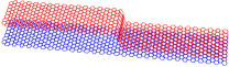
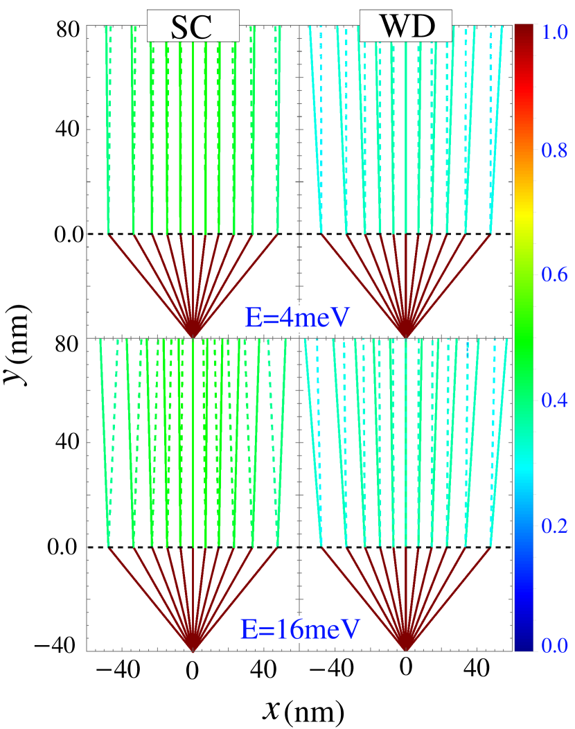
Figure 4: (Color online) Scattering from 2SLG into lower $T_{+}$ (solid lines) and upper $T_{-}$ (dashed lines) cones in AA-BLG with different incident energies. Both 2SLG and AA-BLG are pristine where left and right columns show trajectories obtained from SC and WD approaches, respectively. Color bar represents the transmission probability where $R+T=1$ and $T=T_{+}+T_{-}$.

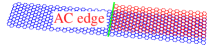
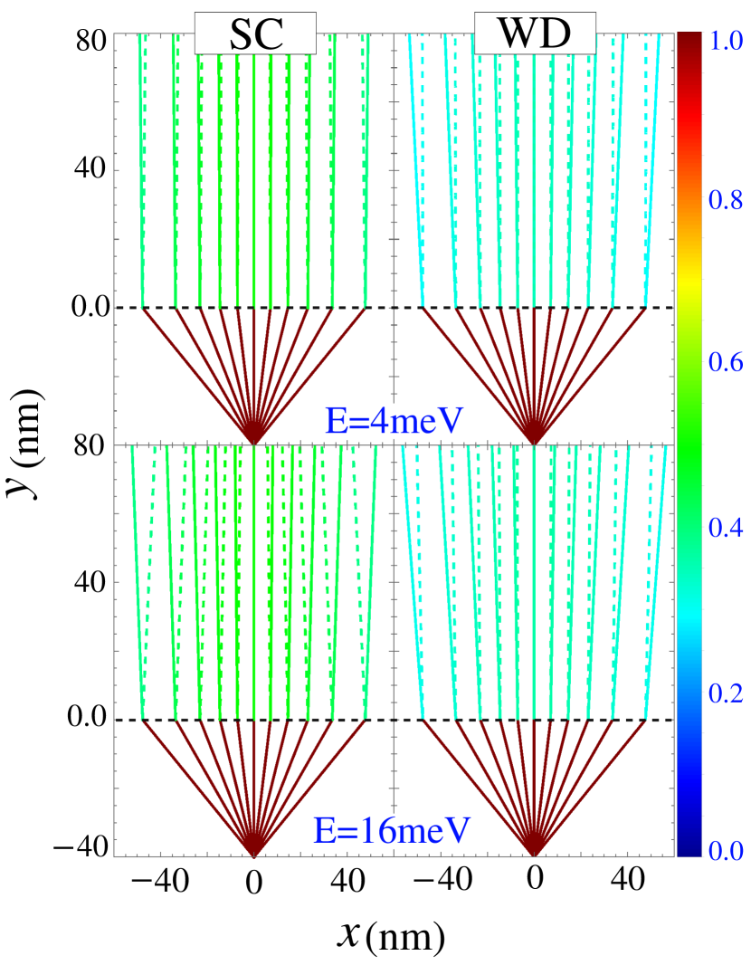
Figure 5: (Color online) The same as in Fig. 4, but the scattering here is from SLG to AA-BLG, whose top layer possesses armchair edge at the interface.

The initial wave packet is taken as a circularly symmetric Gaussian distribution, multiplied by a four spinor in atomic orbital basis $[\psi_{A1},\psi_{B1},\psi_{A2},\psi_{B2}]^{T}$ and by a plane wave with wave vector $\boldsymbol{k}=(k_{x},k_{y})$, which gives the wave packet a non-zero average momentum, defined as

$${\bf\Psi}(\boldsymbol{r},t=0)=N\left(\begin{array}[]{c}\psi_{A1}\\ \psi_{B1}\\ \psi_{A2}\\ \psi_{B2}\end{array}\right)\exp\left[{-\frac{(x-x_{0})^{2}+(y-y_{0})^{2}}{2d^{2}}+i\boldsymbol{k}\cdot\boldsymbol{r}}\right],$$ (15)

where $N$ is a normalization factor, $(x_{0},y_{0})$ are the coordinates of the initial position of center of the Gaussian wave packet, and $d$ is its width. For all studied cases, the width of the Gaussian wave packet was taken as $d=10$ nm and its initial position as $(x_{0},y_{0})=(0,-40)$ nm.

The propagation direction is determined by the pseudospin polarization of the wave packet and plays an important role in defining the direction of propagation. It is characterized by the pseudospin polarization angle $\Theta$, such as $\left(1\mbox{~{},~{}}e^{i\Theta}\right)^{T}$ for the components in each layer. The choice of the angle $\Theta$ depends also on which energy valley the initial wave packet is situatedChaves2015 ; Rakhimov2011 ; Chaves2010 ; da_Costa_2015 ; Costa2012 ; Costa2017 . Our choice for the propagation direction here is based on the knowledge reported in literature for wave packet time evolution on monolayerRakhimov2011 ; Chaves2010 ; Costa2012 and bilayerda_Costa_2015 graphene systems and the consequences of the Zitterbewegung effect on the wave packet trajectoryMaksimova2008 . We assume the $y$-direction as the preferential propagation direction, since the average position of electronic motion along this direction is less affected by the oscillatory behavior caused by the Zitterbewegungda_Costa_2015 .

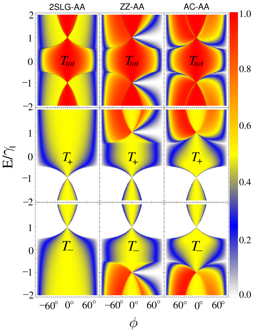
Figure 6: (Color online) Comparison between the transmission probabilities obtained from the SC approach for 2SLG-AA and SLG-AA with zigzag- and armchair-edges with $v_{0}=0$. $T_{+}$ and $T_{-}$ are the cone transmission probabilities where carriers scatter into the lower and upper cones, respectively.

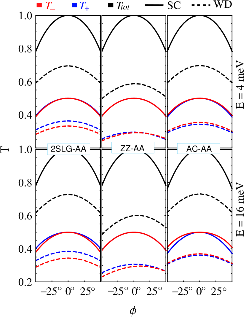
Figure 7: (Color online) Comparison between the transmission probabilities obtained from the wave packet dynamics (WD) and semi-classical approach (SC). The incident energies are $4$ and $16$ meV for top and bottom rows, respectively, while the electrostatic potentialis $v_{0}=0$.

The initial wave vector is taken in the vicinity of the Dirac point $\boldsymbol{k}=(k_{x},k_{y})+\boldsymbol{K}$, where $\boldsymbol{K}=(0,\pm 4\pi/(3\sqrt{3a}))$ represents the two non-equivalent $K$ and $K^{\prime}$ points. As we intend to investigate the wave packet trajectories for different propagation angles and their probabilities, we run the simulation for each system configuration, such as e.g. initial propagation angle, initial wave vector and energy, and then as the Gaussian wave packet propagates, we calculate for each time step the amount of transmission ($T(t)$) and reflection ($R(t)$) and find the electron after $(y>0)$ and before $(y<0)$ the interface at $y=0$, respectively, as the integral of the square modulus of the normalized wave packet in that region, given by

$$T(t) =\int_{-\infty}^{\infty}dx\int_{0}^{\infty}dy|\mathbf{\Psi}(x,y,t)|^{2},$$ (16a)

$$R(t) =\int_{-\infty}^{\infty}dx\int_{-\infty}^{0}dy|\mathbf{\Psi}(x,y,t)|^{2},$$ (16b)

and the total average position, i.e. the trajectory of the center of mass $\langle\boldsymbol{r}\rangle$ of the wave packet, that is calculated for each time step by computing

$$\langle x(t)\rangle =\int_{-\infty}^{\infty}dx\int_{-\infty}^{\infty}dy|\Psi(x,y,t)|^{2}x,$$ (17a)

$$\langle y(t)\rangle =\int_{-\infty}^{\infty}dx\int_{-\infty}^{\infty}dy|\Psi(x,y,t)|^{2}y.$$ (17b)

For larger $t$, the value of the transmission (reflection) probability integral increases (decreases) with time until it converges to a number. This number is then considered to be the transmission (reflection) probability of such system configuration, i.e. $T=T(t\rightarrow\infty)$ ($R=R(t\rightarrow\infty)$).

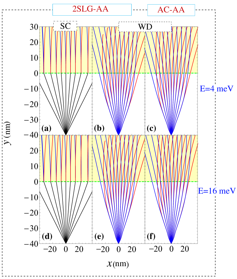
Figure 8: (Color online) SC and WD classical trajectories of the charge carriers scattering from 2SLG into AA-BLG and from SLG into AA-BLG with AC-edge in the presence of a perpendicular magnetic field $B=1$T (only in the yellow region $y$>40 nm) in the $x-y$ plane with $v_{0}=0$ and at different Fermi energies. SC gives the same results for both systems (left column), while WD provides a slight difference for 2SLG-AA and AC-AA (middle and right columns). Red and blue trajectories correspond to scattering into the upper $k^{-}$ and lower $k^{+}$ cones in AA-BLG as indicated in the top of Fig. 2(c).

Note that, essentially, a wave packet is actually a linear combination of plane-waves, where the wave packet width represents a distribution of momenta and, consequently, of energy. In this sense, we are investigating the dynamics of a distribution of plane-waves with different energies around some average value, whose width can be even related e.g. to the temperature of the system. A large wave packet in real space implies a narrow wave packet in $k$-space, thus it will be composed of a distribution of plane-waves with different velocities and, therefore, exhibits a strong decay in time. We have checked that the wave packet width in real space considered in our calculations is appropriate for the proposed problem, being large enough to avoid significant changes of the wave packet within the time scale of interest.

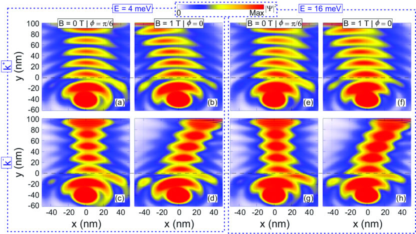
Figure 9: (Color online) Contour plots of the time evolution for the squared modulus of the Gaussian wave function scattering from 2SLG into AA-stacked BLG with an initial energy (a-b) $E=4$ meV and (e-h) $E=16$ meV, for an incident angle $\phi=\pi/6$. The magnetic field was assumed to be (a, c, e, g) $B=0$ and (b, d, f, h) $B=1$ T. Solid-dashed black line indicates the interface of the junction. Top (bottom) panels correspond to the lower $k^{+}$ (upper $k^{-}$) cones in the AA-BLG spectrum.

As mentioned before, the propagation of charge carriers in AA-BLG can be described as belonging to the upper or lower cone, respectively denoted by red and blue in Fig. 1(d). In order to investigate the wave packet scattering to these upper and lower Dirac cones $k^{+}$ and $k^{-}$, one can find a unitary transformation $U$ that block-diagonalizes our Hamiltonian in Eq. (1), such transformation reads

$$U=\frac{1}{\sqrt{2}}\left(\begin{tabular}[]{cccc}$1$&$0$&$1$&$0$\\ $0$&$1$&$0$&$1$\\ $1$&$0$&$-1$&$0$\\ $0$&$1$&$0$&$-1$\end{tabular}\right).$$ (18)

Applying this to the four-spinor in Eq. (15) forms symmetric and antisymmetric combinations of the top and bottom layer wave functions components, i.e.

$$U\mathbf{\Psi}=\mathbf{\Psi}^{\prime}=\frac{1}{\sqrt{2}}\left(\begin{tabular}[]{ccc}$\psi_{A2}+\psi_{A1}$\\ $\psi_{B2}+\psi_{B1}$\\ $\psi_{A2}-\psi_{A1}$\\ $\psi_{B2}-\psi_{B1}$\end{tabular}\right).$$ (19)

The symmetric and antisymmetric components correspond to the $k^{+}$ and $k^{-}$ energy bands (For more details see Refs. [Abdullah2017, ]). In our results for AA-BLG case, we use the above wave function to calculate the center mass position and the probability amplitudes.

III Results and discussions

III.1 Without magnetic field

Before we proceed to show the electron collimation in different systems, we would like to remind the reader of the following: there are three different junctions under consideration, namely, 2SLG-AA, ZZ-AA, and AC-AA. For the SC, the classical trajectories in the three configurations are the same since they depend only on the radius of the Fermi circle on both sides of the junction. However, the transmission probability associated with each system is indeed different. On the other hand, for WD the electron trajectories and transmission probability are distinct in 2SLG-AA and AC-AA, while the results for ZZ-AA are strongly obscured due to the strong Zitterbewegung effect along the zigzag edge as discussed in Sec. II.3.

Additionally, the fact that the lower and upper cones in AA-BLG are decoupled means that each cone exhibits electron- and hole-like carriers. For example, for $\gamma_{1}>E>0$ electron- and hole-like carriers emerge from the lower and upper cones, respectively. Consequently, there will be two different types of collimated beams coming from the two cones as will henceforth be seen.

In Fig. 4 we show the carrier collimation through a domain wall that separates 2SLG and AA-BLG obtained from both SC and WD calculations with different Fermi energies. The point source is positioned at $(x,y)=(0,y_{0})$ nm and electrons impinge on the domain wall located at the origin ($y=0$), afterwards they scatter to either lower (solid) or upper (dashed) cones with different transmission angles. Both approaches show a strong agreement for carrier trajectories. For example, according to SC the refraction index associated with the upper cone for $E=4$ meV is $n=-0.0041$ while the WD calculations give $n=-0.0039$. The plus and minus signs of the refraction index reveal that the respective charge carriers will diverge and converge, respectively, at large distance. The transmission probabilities obtained from the two approaches agreed qualitatively as will be explained later. Experimentally, it is often found that some islands in a sample have single layer graphene connected to bilayer graphene flakesYan2016 ; Clark_2014 . In Fig. 5, we show the carrier trajectories through such structure. We notice that even though the transmission probabilities are slightly altered, the system still attains collimation. We can say that the results are almost identical for 2SLG-AA and AC-AA as depicted in Figs. (4, 5), respectively.

To validate this understanding and quantitatively determine the degree of agreement, we next carry out a transmission comparison between different systems and approaches. Using the SC approach, we show in Fig. 6 the cone as well as the total transmission probabilities in 2SLG-AA, ZZ-AA, and AC-AA systems. In the cone channels $T_{+}$ and $T_{-}$, the charge carriers scatter from SLG region into the lower and upper cones, respectively. In 2SLG-AA system, the transmission is symmetric with respect to normal incidence, while it becomes asymmetric in ZZ-AA and AC-AA systems at high energy. Such an asymmetry feature is a manifestation of breaking the inversion symmetry in the system. Notice that the transmission remains symmetric in the $E-\phi$ regions where both modes $k^{+}$ and $k^{-}$ are propagating and the asymmetry feature only appears when one of them becomes evanescent. The critical energy that separates these two domains are given by $E_{c}^{\pm}(\phi)=\pm\gamma_{1}/(1+\sin\phi)$ and is superimposed as dashed-black curves on $T_{tot}$ in Fig. 6. The critical energy decreases with increasing incident angle which reaches $E_{c}^{\pm}=\pm\gamma_{1}/2$ for $\phi=\pi/2$. Therefore, within this energy range, the electron beam is symmetrically collimated. Moreover, within the same energy range the intensity of the collimated beam is almost the same for all systems. Note that in the other valley $K^{\prime}$ the total transmission probability in ZZ-AA and AC-AA attains the following symmetry $T_{K}(\phi)=T_{K^{\prime}}(-\phi)$. Note that if the edge crosses the lattice at arbitrary angle then such edge would be a mixed edge such that it is locally posses ZZ and AC boundaries. Since the transmission probabilities of both types are almost the same for low energies, we can safely assume that the mixed edge will not significantly alter the transmission probability and thus collimation is maintained since since the radius of Fermi circles in both sides of the junction remains unchanged regardless the edge type.

For comparison with the WD calculations, we show in Fig. 7 the transmission probabilities as a function of the incident angle at two different energies. The fundamental characteristics of the system are qualitatively captured by both approaches. Of particular importance is the deviation in the cone transmission at higher incident angles in 2SLG-AA and AC-AA. At normal incidence and in the SC picture, the cone channels are equal, such that $T_{+}=T_{-}=1/2$, while for oblique angles they start deviating from each other. For 2SLG-AA junction, we notice that $T_{+}>T_{-}$ while it is reversed for AC-AA as can be inferred from the solid blue and red curves in Fig. 7. This behaviour is also captured by the WD as can be seen from the dashed blue and red curves. For ZZ-AA, the WD results for the transmission profile is asymmetric with respect to normal incidence. The reason for this is that the energy tail of the wave packet reaches the region where one of the modes is evanescent as we explained earlier. Furthermore, it is clear that transmission amplitudes from SC and WD do not match precisely. For example, at normal incidence $T_{\rm{tot}}$ is always unity for all systems according to SC, while it is significantly reduced in WD. The reason for this difference is due to the fact that we consider a plane wave in SC approach with single energy and momentum value. In contrasts WD uses a wave packet that defines a burst of particles with a momenta distribution $\hbar\Delta k_{x}$. Thus a perfect transmission is not expected since only part of the wave packet coincides with normal incidence which will be completely transmitted. While the part associated with $k_{x}\neq 0$ will be partially transmitted and reflectedRakhimov2011 .

III.2 With magnetic field

So far, we have shown the electron collimation through different configurations in the absence of a magnetic field. Gaining control over the direction of the electron beams can be realized through a magnetic field without losing collimation. To examine the effect of the magnetic field on the collimated beams, we assume that the magnetic field is applied only in AA-BLG region, i.e. for $y>0$. This can be justified by considering that the electron point source is located near the domain wall such that the distance is much smaller than $r^{c}_{SL}$. Note that even if a global magnetic field is subject to the system, the directional collimation will be maintained as long as $r^{c}_{SL}\gg\left|y_{0}\right|$. To assess the effect of the magnetic field, we calculate the classical trajectories in 2SLG-AA and AC-AA using SC and WD as shown in Fig. 8. We consider an electron beams with maximum incidence angles $\phi=\pm 50^{o}$. The essence of SC approach lies in expressing the relative refraction index $n$ in terms of the wave vectors on both sides of the domain wall. Consequently, the classical trajectories for all considered configurations in the current paper are the same; thus, we show in Fig. 8. the trajectories for only 2SLG-AA. This is also confirmed by the WD calculation where it shows that the trajectories for 2SLG-AA and AC-AA are almost the same, see Figs. 8(b,c) and (e,f). Both SC and WD show contributions from two types of trajectories which is a direct consequence of the electron- and hole-like nature of the carriers associated with the lower and upper cones, respectively. The two trajectories are steered by the magnetic field in diametrically opposite directions.

Finally, to clearly visualize the effect of the magnetic field on the whole wave packet, we show in Fig. 9 the contour plots of the time evolution for the squared modulus of the Gaussian wave for 2SLG-AA. We set the incidence angle to be $\phi=0$ and $\phi=30^{o}$ and show the scattering to each cone separately in the presence and absence of magnetic field, respectively. For $B=0$, once the wave packet reaches the domain wall it starts moving nearly along the $y-$direction, see Figs. 9(a, c) and (e, g) and compare with the trajectories in Fig. 4. In the presence of a magnetic field, the wave packets corresponding to lower and upper cones are steered in different directions without losing collimation. Note that due its spatial spread the wave packet feels the magnetic field before its center reaches the interface and this is clearly seen in Fig. 8. Such behaviour is a manifestation of the quantum non-locality nature of the charge carriers in graphene.

It is important to point up that within the tight-binding model, the effects like the Landau levels in the presence of a perpendicular magnetic field are already embedded in the model, such that we do not need to take nothing more in consideration to take this issue into account, as well as, regardless of the value of the chosen magnetic field, the tight-binding model in the WD simulation takes into account all the consequences of its inclusion. Therefore, for convenience we chose such magnetic field values in order to consider a slightly smaller BLG sample, since it can become computationally expensive for larger structures, keeping in mind that enlarging the sample by a factor $\beta$ will result in a similar collimation effect when reducing the magnetic field by a factor $1/\beta$.

IV conclusion

In conclusion, we have studied electron scattering through locally delaminated AA-BLG systems with two different domain walls. Within the mesoscopic limit where electron current is well approximated by classical trajectories, we presented the SC model that combines quantum mechanical calculations of the transmission probabilities with classical trajectories. To validate the SC approach, we carried out the WD calculations and showed that transmission probabilities and classical trajectories are matching the SC ballistic predictions. The SC model takes advantage of representing the refraction index in terms of the wave vectors on both sides of the domain wall. This results in identical trajectories for the two considered domain walls whose transmission probabilities are indeed different. Within specific energy range, electrons can be highly collimated through the considered system and steered by a magnetic field regardless the types edges and domain walls. Most importantly, the considered system here is free of sharp electrostatic potential steps necessary for Klein tunneling and thus electron collimation. However, the major challenge in the experimental realization remains achieving SLG-AA domain walls which can be feasible in the near future as a result of the continued and decent development of graphene samples quality. Finally, we hope that our results will prove useful for designing graphene-based collimation optical devices that enable a new class of transport measurements.

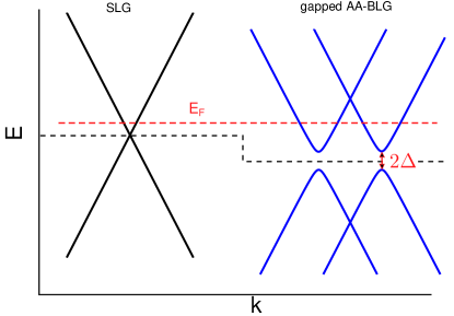
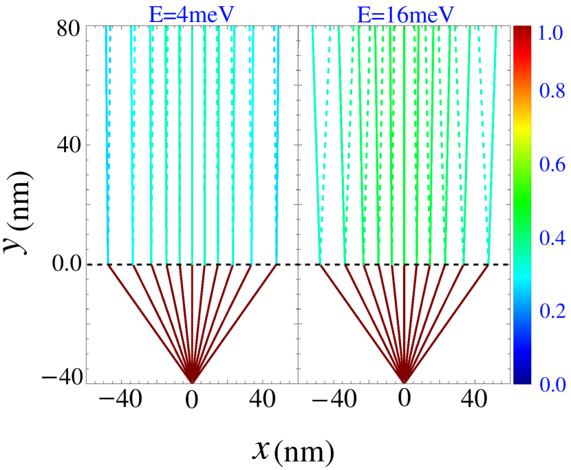
Figure 10: (Color online) Top: energy bands of SLG and gapped AA_BLG, dashed-black line represents the electrostatic potential $v_{0}$. Bottom: SC electron collimation as in Fig. 4 but for gAA with $2\Delta=0.2\gamma_{1}$ and $v_{0}=-2\Delta$. Note that for the other configurations the collimation is the same but the transmission probability will be slightly different.

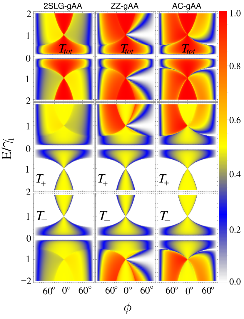
Figure 11: (Color online) Cone and total transmission probabilities for gapped AA-BLG for the three considered configurations 2SLG-gAA, ZZ-gAA, and AC-gAA as in Fig. 6 with $v_{0}=0$ and a gap of magnitude $2\Delta=0.2\gamma_{1}$.

Appendix A gapped AA-stacked bilayer graphene

Through this paper we considered pristine AA-BLG whose spectrum is gapless and compose of two Dirac cones separated by $2\gamma_{1}$. However, the more realistic spectrum is gapped due to the electron-electron interaction in grapheneRakhmanov_2012 ; Sboychakov_2013 ; Brey2013 . In this appendix we show that the electron collimation reported in this paper is maintained even in the presence of a finite gap in AA-BLG energy spectrum.

In fact, the main effect of the gap coincides only with a slight change in the transmission probabilities. For the gapped AA-BLG (gAA), the continuum approximation for the Hamiltonian that describes the electrons in the vicinity of the K-valley readsAbdullah2018c ; Tabert2012

$$\mathcal{H}=\left(\begin{array}[]{cccc}\Delta+v_{0}&v_{F}\pi^{{\dagger}}&\gamma_{1}&0\\ v_{F}\pi&-\Delta+v_{0}&0&\gamma_{1}\\ \gamma_{1}&0&-\Delta+v_{0}&v_{F}\pi^{{\dagger}}\\ 0&\gamma_{1}&v_{F}\pi&\Delta+v_{0}\\ \end{array}\right).$$ (20)

The electron-electron interaction breaks the layer and sublattice symmetries which results in the finite gap of magnitude 2$\Delta$ in the energy spectrumRozhkov_2016 , see top panel of Fig. 10. To investigate the collimation at the same Fermi energy considered in the case of pristine AA-BLG, we subject the gAA to an electrostatic gate $v_{0}$ as presented by the dashed black line in the top panel of Fig. 10. Then, we perform the same steps discussed in Sec. II.2 to calculate the electron collimation in gAA. In the bottom of Fig. 10 we show the electron collimation obtained using SC approach for two different Fermi energies. We consider a gap of magnitude $2\Delta=0.2\gamma_{1}$ and an electrostatic gate of strength $v_{0}=-2\Delta$. It appears that the collimation is preserved even in the presence of a finite energy gap, see Fig. 4 for comparison. This due to the fact that the electron collimation is always preserved as long as the radius of the Fermi circle in AA-BLG region is much larger than its counterpart in SLG. Introducing the gap does not significantly alter the radius of the Fermi circle; however, the transmission probabilities are slightly reduced. In Fig. 11 we show the cone and total transmission probabilities in gAA for three configurations 2SLG-gAA, ZZ-gAA, and AC-gAA. As a comparison with the results for pristine AA-BLG., we see that the transmission probability is drastically altered for energies around the induced gap. It is completely suppressed within the energy gap but apart from the gap and within the symmetric zones the transmission probabilities are comparable for both systems. Another difference is that as a results of braking the inversion symmetry the transmission probability for 2SLG-gAA is asymmetric with respect to normal incidence. In conclusion, electron collimation can be preserved in both pristine and gapped AA-BLG, the only difference is that the latter one is not free of electrostatic gate.

References

- (1) V. V. Cheianov, V. Fal'ko, and B. L. Altshuler, Science 315, 1252 (2007).
- (2) L. Banszerus, M. Schmitz, S. Engels, M. Goldsche, K. Watanabe, T. Taniguchi, B. Beschoten, and C. Stampfer, Nano Lett. 16, 1387 (2016).
- (3) K. Wang, M. M. Elahi, K. M. M. Habib, T. Taniguchi, K. Watanabe, A. W. Ghosh, G.-H. Lee, and P. Kim, http://arxiv.org/abs/1809.06757v2.
- (4) U. Sivan, M. Heiblum, C. P. Umbach, and H. Shtrikman, Phys. Rev. B 41, 7937 (1990).
- (5) W. D. Oliver, Science 284, 299 (1999).
- (6) R. R. Hartmann, N. J. Robinson, and M. E. Portnoi, Phys. Rev. B 81, 245431 (2010).
- (7) J. R. Williams, T. Low, M. S. Lundstrom, and C. M. Marcus, Nat. Nanotechnol. 6, 222 (2011).
- (8) K. S. Novoselov, A. K. Geim, S. V. Morozov, D. Jiang, Y. Zhang, S. V. Dubonos, I. V. Grigorieva, and A. A. Firsov, Science 306, 666 (2004).
- (9) A. K. Geim, and K. S. Novoselov, Nat. Mater. 6, 183 (2007).
- (10) C. W. J. Beenakker, Rev. Mod. Phys. 80, 1337 (2008).
- (11) O. Klein, Zeitschrift für Physik 53, 157 (1929).
- (12) N. Stander, B. Huard, and D. Goldhaber-Gordon, Phys. Rev. Lett. 102, 026807 (2009).
- (13) M. I. Katsnelson, K. S. Novoselov, and A. K. Geim, Nat. Phys. 2, 620 (2006).
- (14) C. Gutiérrez, L. Brown, C.-J. Kim, J. Park, and A. N. Pasupathy, Nat. Phys. 12, 1069 (2016).
- (15) H. M. Abdullah, and H. Bahlouli, J. Comput. Sci. 26, 135 (2018).
- (16) G.-H. Lee, G.-H. Park, and H.-J. Lee, Nat. Phys. 11, 925 (2015).
- (17) S. Chen, Z. Han, M. M. Elahi, K. M. M. Habib, L. Wang, B. Wen, Y. Gao, T. Taniguchi, K. Watanabe, J. Hone, A. W. Ghosh, and C. R. Dean, Science 353, 1522 (2016).
- (18) V. G. Veselago, Sov. Phys. Usp. 10, 509 (1968).
- (19) P. V. Parimi, W. T. Lu, P. Vodo, J. Sokoloff, J. S. Derov, and S. Sridhar, Phys. Rev. Lett. 92, 127401 (2004).
- (20) E. Cubukcu, K. Aydin, E. Ozbay, S. Foteinopoulou, and C. M. Soukoulis, Phys. Rev. Lett. 91, 207401 (2003).
- (21) J. C. W. Song, and N. M. Gabor, Nature Nanotechnology 13, 986 (2018).
- (22) A. A. Houck, J. B. Brock, and I. L. Chuang, Phys. Rev. Lett. 90, 137401 (2003).
- (23) A. Grbic, and G. V. Eleftheriades, Phys. Rev. Lett. 92, 117403 (2004).
- (24) K. E. Aidala, R. E. Parrott, T. Kramer, E. J. Heller, R. M. Westervelt, M. P. Hanson, and A. C. Gossard, Nat. Phys. 3, 464 (2007).
- (25) S. W. LaGasse, and J. U. Lee, Phys. Rev. B 95, 155433 (2017).
- (26) S.-H. Zhang, W. Yang, and F. M. Peeters, Phys. Rev. B 97, 205437 (2018).
- (27) M. Sanderson, Y. S. Ang, and C. Zhang, Phys. Rev. B 88, 245404 (2013).
- (28) C. G. Péterfalvi, L. Oroszlány, C. J. Lambert, and J. Cserti, New J. Phys. 14, 063028 (2012).
- (29) C.-H. Park, Y.-W. Son, L. Yang, M. L. Cohen, and S. G. Louie, Nano Lett. 8, 2920 (2008).
- (30) S. K. Choi, C.-H. Park, and S. G. Louie, Phys. Rev. Lett. 113, 026802 (2014).
- (31) M.-H. Liu, C. Gorini, and K. Richter, Phys. Rev. Lett. 118, 066801 (2017).
- (32) A. W. Barnard, A. Hughes, A. L. Sharpe, K. Watanabe, T. Taniguchi, and D. Goldhaber-Gordon, Nat. Commun. 8, 15418 (2017).
- (33) S. Bhandari, G. H. Lee, K. Watanabe, T. Taniguchi, P. Kim, and R. M. Westervelt, 2D Mater. 5, 021003 (2018).
- (34) C. Handschin, B. Fülöp, P. Makk, S. Blanter, M. Weiss, K. Watanabe, T. Taniguchi, S. Csonka, and C. Schönenberger, Appl. Phys. Lett. 107, 183108 (2015).
- (35) A. Kinikar, T. P. Sai, S. Bhattacharyya, A. Agarwala, T. Biswas, S. K. Sarker, H. R. Krishnamurthy, M. Jain, V. B. Shenoy, and A. Ghosh, Nat. Nanotechnol. 12, 564 (2017).
- (36) H. Overweg, H. Eggimann, X. Chen, S. Slizovskiy, M. Eich, R. Pisoni, Y. Lee, P. Rickhaus, K. Watanabe, T. Taniguchi, V. Fal’ko, T. Ihn, and K. Ensslin, Nano Lett. 18, 553 (2017).
- (37) P. Bøggild, J. M. Caridad, C. Stampfer, G. Calogero, N. R. Papior, and M. Brandbyge, Nat. Commun. 8, 15783 (2017).
- (38) H. M. Abdullah, B. Van Duppen, M. Zarenia, H. Bahlouli, and F. M. Peeters, J. Phys.: Condens. Matter 29, 425303 (2017).
- (39) H. M. Abdullah, M. Van der Donck, H. Bahlouli, F. M. Peeters, and B. Van Duppen, Appl. Phys. Lett. 112, 213101 (2018).
- (40) H. M. Abdullah, H. Bahlouli, F. M. Peeters, and B. Van Duppen, J. Phys.: Condens. Matter 30, 385301 (2018).
- (41) H. M. Abdullah, M. Zarenia, H. Bahlouli, F. M. Peeters, and B. Van Duppen, Europhys. Lett. 113, 17006 (2016).
- (42) T. L. M. Lane, M. Anđelković, J. R. Wallbank, L. Covaci, F. M. Peeters, and V. I. Fal'ko, Phys. Rev. B 97, 045301 (2018).
- (43) M. Mirzakhani, M. Zarenia, S. A. Ketabi, D. R. da Costa, and F. M. Peeters, Phys. Rev. B 93, 165410 (2016).
- (44) K. Reijnders, T. Tudorovskiy, and M. Katsnelson, Ann. Phys. 333, 155 (2013).
- (45) S. P. Milovanović, D. Moldovan, and F. M. Peeters, J. Appl. Phys. 118, 154308 (2015).
- (46) K. J. A. Reijnders, and M. I. Katsnelson, Phys. Rev. B 95, 115310 (2017).
- (47) S. P. Milovanović, M. R. Masir, and F. M. Peeters, J. Appl. Phys. 115, 043719 (2014).
- (48) G. M. Maksimova, V. Y. Demikhovskii, and E. V. Frolova, Phys. Rev. B 78, 235321 (2008).
- (49) A. Chaves, L. Covaci, K. Y. Rakhimov, G. A. Farias, and F. M. Peeters, Phys. Rev. B 82, 205430 (2010).
- (50) V. Krueckl, and T. Kramer, New J. Phys. 11, 093010 (2009).
- (51) F. Zhang, J. Jung, G. A. Fiete, Q. Niu, and A. H. MacDonald, Phys. Rev. Lett. 106, 156801 (2011).
- (52) Z. Q. Li, E. A. Henriksen, Z. Jiang, Z. Hao, M. C. Martin, P. Kim, H. L. Stormer, and D. N. Basov, Phys. Rev. Lett. 102, 037403 (2009).
- (53) Y. Xu, X. Li, and J. Dong, Nanotechnology 21, 065711 (2010).
- (54) I. Lobato, and B. Partoens, Phys. Rev. B 83, 165429 (2011).
- (55) A. H. Castro Neto, F. Guinea, N. M. R. Peres, K. S. Novoselov, and A. K. Geim, Rev. Mod. Phys. 81, 109 (2009).
- (56) T. Nakanishi, M. Koshino, and T. Ando, Phys. Rev. B 82, 125428 (2010).
- (57) M. Barbier, P. Vasilopoulos, and F. M. Peeters, Phys. Rev. B 82, 235408 (2010).
- (58) B. Van Duppen, and F. M. Peeters, Phys. Rev. B 87, 205427 (2013).
- (59) H. M. Abdullah, A. E. Mouhafid, H. Bahlouli, and A. Jellal, Mater. Res. Express 4, 025009 (2017).
- (60) J. M. Pereira, F. M. Peeters, A. Chaves, and G. A. Farias, Semicond. Sci. Technol. 25, 033002 (2010).
- (61) M. R. Masir, P. Vasilopoulos, and F. M. Peeters, Phys. Rev. B 82, 115417 (2010).
- (62) M. Barbier, P. Vasilopoulos, and F. M. Peeters, Phil. Trans. R. Soc. A 368, 5499 (2010).
- (63) S. Park, and H.-S. Sim, Phys. Rev. B 84, 235432 (2011).
- (64) V. T. Phong, and J. F. Kong, arXiv: 1610.00201v1 (2016).
- (65) V. Ariel, and A. Natan, Electron effective mass in graphene, in 2013 International Conference on Electromagnetics in Advanced Applications (ICEAA), IEEE, 2013.
- (66) N. W. Ashcroft, and N. D. Mermin, Solid State Physics (Cengage Learning, Boston, 1976), pp. 231–233.
- (67) K. Zou, X. Hong, and J. Zhu, Phys. Rev. B 84, 085408 (2011).
- (68) F. Batista, A. Chaves, D. R. da Costa, and G. Farias, Physica E 99, 304 (2018).
- (69) D. R. da Costa, A. Chaves, G. A. Farias, and F. M. Peeters, J. Phys.: Condens. Matter 29, 215502 (2017).
- (70) A. Chaves, D. R. da Costa, G. O. de Sousa, J. M. Pereira, and G. A. Farias, Phys. Rev. B 92, 125441 (2015).
- (71) L. S. Cavalcante, A. Chaves, D. R. da Costa, G. A. Farias, and F. M. Peeters, Phys. Rev. B 94, 075432 (2016).
- (72) D. R. da Costa, A. Chaves, G. A. Farias, L. Covaci, and F. M. Peeters, Phys. Rev. B 86, 115434 (2012).
- (73) D. R. da Costa, A. Chaves, S. H. R. Sena, G. A. Farias, and F. M. Peeters, Phys. Rev. B 92, 045417 (2015).
- (74) A. Chaves, G. A. Farias, F. M. Peeters, and B. Szafran, Phys. Rev. B 80, 125331 (2009).
- (75) M. H. Degani, and M. Z. Maialle, J. Comput. Theor. Nanosci. 7, 454 (2010).
- (76) A. Chaves, G. A. Farias, F. M. Peeters, and R. Ferreira, Comm. Comput. Phys. 17, 850 (2015).
- (77) K. Y. Rakhimov, A. Chaves, G. A. Farias, and F. M. Peeters, J. Phys.: Condens. Matter 23, 275801 (2011).
- (78) T. Kramer, AIP Conf. Proc. 1334, 142 (2011).
- (79) W. Yan, S.-Y. Li, L.-J. Yin, J.-B. Qiao, J.-C. Nie, and L. He, Phys. Rev. B 93, 195408 (2016).
- (80) K. W. Clark, X.-G. Zhang, G. Gu, J. Park, G. He, R. M. Feenstra, and A.-P. Li, Phys. Rev. X 4, 011021 (2014).
- (81) A. L. Rakhmanov, A. V. Rozhkov, A. O. Sboychakov, and F. Nori, Phys. Rev. Lett. 109, 206801 (2012).
- (82) A. O. Sboychakov, A. L. Rakhmanov, A. V. Rozhkov, and F. Nori, Phys. Rev. B 87, 121401(R) (2013).
- (83) L. Brey, and H. A. Fertig, Phys. Rev. B 87, 115411 (2013).
- (84) H. M. Abdullah, M. A. Ezzi, and H. Bahlouli, J. Appl. Phys. 124, 204303 (2018).
- (85) C. J. Tabert, and E. J. Nicol, Phys. Rev. B 86, 075439 (2012).
- (86) A. Rozhkov, A. Sboychakov, A. Rakhmanov, and F. Nori, Phys. Rep. 648, 1 (2016).