Crack propagation under static and dynamic boundary conditions

Abstract

Velocity jumps observed for crack propagation under a static boundary condition have been used as a controlling factor in developing tough rubbers. However, the static test requires many samples to detect the velocity jump. On the contrary, crack propagation performed under a dynamic boundary condition is timesaving and cost-effective in that it requires only a single sample to monitor the jump. In addition, recent experiments show that velocity jump occurs only in the dynamic test for certain materials, for which the velocity jump is hidden in the static test because of the effect of stress relaxation. Although the dynamic test is promising because of these advantages, the interrelation between the dynamic test and the more established static test has not been explored in the literature. Here, by using two simulation models, we elucidate this interrelation and clarify a universal condition for obtaining the same results from the two tests, which will be useful for designing the dynamic test.

I Introduction

Crack propagation is a crucial factor for controlling the toughness of materials. For crack-propagation in elastomers, a remarkable phenomenon, called velocity jump Tsunoda2000 , has recently been revisited and has attracted considerable attention, which include experimental MoridhitaUrayama2016PRE ; morishita2017crack , numerical kubo2017velocity , and analytical sakumichi2017exactly ; Okumura2018 studies. The velocity jump refers to a sharp jump in the velocity of crack propagation, typically from 0.1 mm/s to 1 m/s, as a function of the energy release rate $G$, which is an increasing function of the applied displacement $\varepsilon$. (In the linear case, $G$ is proportional to $\varepsilon^{2}$). The experiment is conventionally performed under a static boundary condition (fixed-grip condition): crack propagation starts at an initial displacement, while the displacement is kept fixed during the crack propagation.

The analytical study sakumichi2017exactly as well as the numerical study kubo2017velocity suggest that the physical origin of the velocity jump is the glass transition at the crack tip KuboSakumichi . The ratio of the velocities before and after the jump is only four orders of magnitude at most, but the region in which glass transition occurs is very localized near the tip, causing a significant reduction in the characteristic length scale; these two effects are combined to attain a significant change (of nearly nine orders of magnitude) in strain rate at the crack tip required for glass transition Okumura2018 .

Recently, it is reported that the velocity jump is not observed for a semi-crystalline polymer Takei2018 as a result of performing the crack-propagation test under the static boundary condition. However, more recently, the velocity jump is successfully observed for the same semi-crystalline polymer when the crack-propagation test is performed under a dynamic boundary condition TomizawaJump2 .

In the dynamic test, the change in the velocity of crack propagation is monitored when the sheet sample is extended at a constant speed in the direction perpendicular to the direction of crack propagation. Because of this dynamic boundary condition, the stress relaxation is minimized in the dynamic test (in the static test, we generally have a preparation time for giving a fixed strain before starting crack propagation), which leads to the observation of the velocity jump. In other words, the dynamic test is more sensitive for detecting the velocity jump for certain polymers and thus applicable to a wider range of materials than the static test.

In addition to this advantage concerning the sensitivity, the dynamic test is timesaving and cost-effective. This is because the dynamic test requires one sample (to be broken) in order to obtain a single point in the velocity-displacement plot. On the contrary, one complete velocity-displacement curve is obtained from a single sample in the dynamic test.

As seen above, the dynamic test has strong advantages over the static test for detecting the velocity jump. However, to date, there have been no studies which discuss the relation between the results obtained from the static and dynamic tests. Here, we elucidate this relation through a numerical study. We use two simple viscoelastic models appropriate for examining crack propagation aoyanagi2017 ; aoyanagiNonlinear . One model is a spring-bead model based on Voigt model. Note that analysis of such a simple model is always important to know the basic properties. The other model is another spring-bead model, in which viscous dissipation is introduced by a friction force proportional to the bead velocity. We show in the Appendix rheological response of the model to show that the model can appropriately describe essential features of polymer rheology. From the results obtained from these two models, we clarify simple and universal conditions under which the two tests provide equivalent information. The results shall be useful for designing the dynamic test as a clever substitute for the static test.

II Simulation models

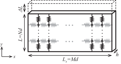
Figure 1: Schematic illustration showing the arrangement of springs and beads in a network structure. $N$ springs are arranged in series in the $y$ direction and $M$ springs in the $x$ direction. Beads are located on nodal points of the springs.

In order to represent the network structure in polymer materials, we consider a simple two dimensional square-lattice network, as shown in Fig. 1. Beads are arranged on nodal points on a square lattice with lattice spacing $d$; each bead is connected to the four nearest neighbors by springs of spring constant $k$. The bead positions initially located at the lattice point $\mathbf{m}=(i,j)$ are labeled by $\mathbf{x}_{\mathbf{m}}$. Let us define the vector $\Delta\mathbf{x}_{\mathbf{mm}^{\prime}}$ as the extension vector from the natural length of spring connecting $\mathbf{m}$ and $\mathbf{m}^{\prime}$ (see Sec. .1 of Appendix for the details, where we introduce the index $s$ ($s=1,2,3,4$), for which $s=1$ and 3 correspond to the shear force and $s=2$ and 4 to the tensile force in the $y$ direction); $\mathbf{m}^{\prime}$ is the index of one of the nearest neighbor sites of the site represented by $\mathbf{m}$.

In the present study, we consider the following two types of equation of motion:

$$\gamma\frac{d}{dt}\Delta\mathbf{x}_{\mathbf{m}}+k\Delta\mathbf{x}_{\mathbf{m}} =\mathbf{F}_{\mathbf{m}}$$ (1)

$$\gamma\frac{d}{dt}\mathbf{x}_{\mathbf{m}}+k\Delta\mathbf{x}_{\mathbf{m}} =\mathbf{F}_{\mathbf{m}}$$ (2)

$$\Delta\mathbf{x}_{\mathbf{m}} =\sum_{{(\mathbf{m}^{\prime})}}\Delta\mathbf{x}_{\mathbf{mm}^{\prime}}$$ (3)

Here, the summation $\sum_{{(\mathbf{m}^{\prime})}}$ stands for the summation over the position indices of the four nearest neighbor beads of the bead initially located at $\mathbf{m}$. Note that $\Delta\mathbf{x}_{\mathbf{m}}$ is nonlocal for the lattice index, and thus the equations of motions in the above couple the dynamics of a bead with its nearest neighbors (see Sec. .1 of Appendix for the details). The force $\mathbf{F}_{\mathbf{m}}$ is the external force acting on the beads at $\mathbf{x}_{\mathbf{m}}$. This force is set to zero except for the case in which we consider the boundary force (as in the case of a creep test). These models describe a strongly viscous case in which the inertial term is neglected and thus the elastic and viscous stress are always balanced in the system when $\mathbf{F}_{\mathbf{m}}=0$.

When we stretch the two-dimensional network in the $y$ direction, we set initially the $x$-component of $\Delta\mathbf{x}_{\mathbf{mm}^{\prime}}$ to zero for simplicity. The $y$ component of the above equations of motion are, respectively, given as

$$\gamma\frac{d}{dt}\Delta y_{\mathbf{m}}+k\Delta y_{\mathbf{m}} =Y_{\mathbf{m}}$$ (4)

$$\gamma\frac{d}{dt}y_{\mathbf{m}}+k\Delta y_{\mathbf{m}} =Y_{\mathbf{m}}$$ (5)

where $\Delta y_{\mathbf{m}}$ and $Y_{\mathbf{m}}$ are the $y$ components of $\Delta\mathbf{x}_{\mathbf{m}}$ and $\mathbf{F}_{\mathbf{m}}$, respectively.

The first case whose dynamics is governed by Eq. (4) will be called the model with a single relaxation time, whereas the second case in Eq. (5) the model with multi relaxation times. This is because as explained in Sec. .2 of Appendix, the former model possesses a single relaxation time $\tau=\gamma/k\,$, whereas the latter has $N$ relaxation times $\tau_{i}=\gamma/(k\lambda_{i})$ with $i=1,\ldots,N$. [As demonstrated in Sec. .2 of Appendix, the maximum of $\tau_{i}$ scales with $N^{\nu}\gamma/k$ where $\nu$ is close to 2 and the minimum approach $(5/16)\gamma/k$ as $N$ increases.] The response to the creep test of the first model is equivalent to that of Voigt model, whereas rheological properties of the second model are similar to those of cross-linked polymers. Further details on rheological aspects are discussed in Sec. .3 of Appendix, in which rheological properties of the two models are examined.

For convenience, we introduce elastic modulus $E$ (of the unit Pa) and viscosity  $\eta$ (of the unit Pa$\cdot$s) through relations $E=k/d$ and $\eta=\gamma/d$. The local strain for a given spring is given by the elongation of the spring divided by the lattice spacing $d$. The global strain for the network is defined as the elongation of the distance between the top and bottom rows $\Delta L$ divided by the original length $L$ (see Fig. 1).

The numerical calculation for crack-propagation tests are performed as follows. In the static test, we first prepare an equilibrium state for the network with an initial (homogeneous) strain in the $y$ direction by giving fixed positions at the top and bottom of the network; second, we introduce a crack of length $a_{0}$ by removing springs from network located at corresponding positions; third, we move each bead in the network on the basis of the equation of motion, i.e., either of eq. (4) or eq. (5), under the condition that any spring in the network is removed if the strain of the spring reaches a critical value $\varepsilon_{c}$.

In the dynamic test under constant-speed stretching at the velocity $U$, we first introduce a crack of length $a_{0}$ in the network system in the unstretched state (in which the length of each spring is equal to its natural length) by removing springs; second, we start to move all the beads at the top row upwards (i.e., in the positive $y$ direction) with the speed $U$, while each bead moves on the basis of the equation of motion under the condition that any spring in the network is removed if the strain of the spring reaches a critical value $\varepsilon_{c}$.

In both cases, we only solve the $y\,$-component equation because the $x$ and $y$ components are decoupled in Eqs. (1) and (2). In addition, we set $Y_{\mathbf{m}}=0$ because the boundary condition is given not by force but by strain in both cases of the static and dynamic tests (when we consider the creep test in Sec. .3 of Appendix, we deal with the case of nonzero $Y_{\mathbf{m}}$).

In the model with multi relaxation times, the extension is transmitted from the top to bottom of the system with time delay (note that the top row is in tension while the bottom is fixed). Concerning this time delay, we confirmed numerically the following property. In the case without crack, i.e., when every column is stretched in the same way, if we introduce the difference between the strains at adjacent (with respect to the $j$ index) rows by $\Delta\varepsilon_{j}=\varepsilon_{j+1}-\varepsilon_{j}$ for the homogeneous (with respect to the $i$ index) strain $\varepsilon_{j}=y_{i,j+1}-y_{i,j}$, this quantity $\Delta\varepsilon_{j}$ satisfies the relation $\Delta\varepsilon_{j}=\eta Uj/(NE)$. This implies that if the quantity $\eta U/(NE)$ is not small enough, it is possible that the strain of the spring at the top $\varepsilon_{N-1}$ reaches $\varepsilon_{c}$ before the strain at the crack tip does. In such a case, the crack does not propagate from the tip, but the network starts to break near the top row. Analytical expressions for the model concerning related properties, including its rheological functions, will be discussed elsewhere.

III Results and Discussions

The simulation is performed under the standard parameter set $(E,\eta,\varepsilon_{c},L,d)=(100,80,0.32,10,1)$ unless specified (in appropriate dimensionless units; e.g., the unit of $L$ is $d$). The width of the system $W$ and the initial crack size $a_{0}$ are set to $1000d$ and $100d$ by default in both of the simulation models. However, in the dynamic test, when $U$ is relatively large, $W$ is made larger than the default value up to $6000d$ for the global strain to reach $\varepsilon_{c}$ before the crack tip reaches the opposite side edge of the sample (in order to observe the least upper bound discussed below). In the following, we show plots of the crack propagation velocity $V$ as a function of the energy release rate $G$, which is given by $E\varepsilon^{2}L/2$ in the present linear case.

III.1 Model with a single relaxation time

In this section, we compare the results of crack-propagation tests under the static and dynamic boundary conditions obtained from the model with a single relaxation time. We announce here in advance that our numerical results provided below support the following conclusion. If the condition

$$U <U_{c}$$ (6)

$$U_{c} =Ed/\eta$$ (7)

is well satisfied the static and dynamic tests give the same result. On the contrary, when $U$ does not satisfy this condition, the plot of the crack-propagation speed $V$ as a function of a given strain $\varepsilon$ obtained from the dynamic test tends to shift upwards as $U$ increases. This may be understood as follows. Near the crack tip, the two different dynamics, both tend to increase the strain $\varepsilon$ $(<\varepsilon_{c})$ of the spring at the crack tip, compete with each other: one associated with the relaxation characterized by the time scale $\eta/E$ and the other associated with the strain rate set by the pulling speed $U$ characterized by the time $d/U$. (Note that in the model with a single relaxation time the network is homogeneously stretched if cracks are absent and the stretching motion is characterized by the strain rate $U/d$.) As a result, as long as the relaxation dynamics governs the increase of the strain at the crack tip, which is equivalent to the condition for the time scales $\eta/E<d/U$, the results of the dynamic test become equivalent to those of the static test. In fact, this time-scale condition is identical to the condition given in Eq. (6).

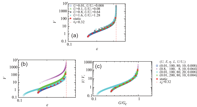
Figure 2: Results from the model with a single relaxation time. (a) $V$ vs $\varepsilon$ for different pulling speed $U$ for the fixed parameter set $(E,\eta,\varepsilon_{c},L,d)=(100,80,0.32,10,1)$, from which $U_{c}$ is estimated as 1.25. (b) $V$ vs $\varepsilon$ for different pulling speed $U$ for the different parameter sets with the condition $U/U_{c}<1$ well satisfied, where $(\varepsilon_{c},d)=(0.32,1)$. (c) The data shown in (b) on the renormalized axes $V/V_{c}$ and $G/G_{c}$.

Now, we confirm the above physical arguments by our numerical data obtained from simulation. In Fig. 2 (a), the relation between the crack-propagation speed $V$ and the global strain of the system $\varepsilon$ are given. The result obtained from the static test is compared with those from the dynamic test performed under different stretching speed $U$. The data are obtained for the same, standard parameter set $(E,\eta,\varepsilon_{c},L,d)=(100,80,0.32,10,1)$. Thus, any differences in the results come from differences in the boundary conditions. As shown in the plot, we confirm that if the condition in Eq. (6) is well satisfied the results from the static and dynamic tests are the same, whereas slight upwards shifts are observed with the increase in $U$ if Eq. (6) is not well satisfied. The reason of shifts in the upwards direction can physically be understood if we remind that the shifts originate from the fact that pulling with the velocity $U$ expedites faster stress concentration at the crack tip.

In Fig. 2 (b) and (c), we show that the above results is not special to the standard parameter set and that the results obtained at a small velocity $U$ which satisfies Eq. (6) well possess the following properties, which the results in the static test were confirmed to satisfy in our previous study aoyanagi2017 ; aoyanagiNonlinear . (A) $V/V_{c}$ is given as a function of $G/G_{c}$, where

$$V_{c} =Ed/\eta$$ (8)

$$G_{c} =E\varepsilon_{c}^{2}L/2$$ (9)

This implies that the $V-\varepsilon$ curves collapse on to a single master curve when plotted on the renormalized axes, $V/V_{c}$ and $G/G_{c}$. The velocity scale $V_{c}$ is given by the smallest length scale $d$ divided by the single time scale of the model $\eta/E$, i.e., $V_{c}$ is the smallest velocity scale of the model. The quantity $G_{c}$ is the value of $G$ evaluated when $\varepsilon$ matches its critical value $\varepsilon_{c}$, i.e., $G_{c}$ is the largest scale of $G$. (B) The greatest lower bound and least upper bound for the $V/V_{c}-G/G_{c}$ relation are characterized by $G_{\min}$ and $G_{\max}$ defined as

$$G_{\min} =c_{1}G_{c}d/L=c_{1}E\varepsilon_{c}^{2}d/2$$ (10)

$$G_{\max} =G_{c}$$ (11)

with a universal numerical coefficient $c_{1}$ (see below). Here, for later convenience, we define $\varepsilon_{0}$ by the following equation:

$$G_{\min}=E\varepsilon_{0}^{2}L/2$$ (12)

It is natural that $G_{\max}$ is given by $G_{c}$ considering that the spring breaks when $\varepsilon=\varepsilon_{c}$. The bound $G_{\min}$ corresponds to the static fracture energy discussed by Lake and Thomas LakeThomas1967 , and also corresponds to the critical state in which the maximum stress at the crack tip coincides with the intrinsic failure $E\varepsilon_{c}$.

In Fig. 2 (b), we show the results obtained from various parameters but with the stretching velocities $U$ all satisfy Eq. (6) well. Although the data in Fig. 2 (b) are scattered, when the same data are replotted on the renormalized axes based on Eqs. (8) and (9), they collapse onto a master curve: the dynamic test has properties (A) and (B), as the static test does. The deviation of the data with $L=20$ in Fig. 2 (c) is consistent with Eq. (10), where $c_{1}$ is approximately 2.3 for all the data shown in Fig. 2. (The constant $c_{1}$ seems weekly dependent on $N$ but takes the same value for the two simulation models for a given $N$; in the previous studies aoyanagi2017 ; aoyanagiNonlinear , $c_{1}$ is approximately 2.4 in the two simulation models for $N=200$, which is about ten times larger than present values of $N$.)

III.2 Model with multi relaxation times

In this section, we compare the results of crack-propagation tests under the static and dynamic boundary conditions obtained from the model with multi relaxation times. We announce here in advance that our numerical results provided below in Fig. 3 support the following properties. If the following condition is well satisfied the static and dynamic tests give the same result:

$$U <U_{c,m}$$ (13)

$$U_{c,m} =U_{c}/N=(Ed/\eta)/N$$ (14)

When $U$ does not satisfy this condition in the dynamic test, the least upper bound and greatest lower bound for the strain $\varepsilon_{\max}$ and $\varepsilon_{\min}$, which are $\varepsilon_{c}$ and $\varepsilon_{0}$ [in Eq. (12)] in the static test, decreases and increases, respectively. These two bounds are given by the following relations as shown in Fig. 3 (d) below:

$$\Delta_{\max} =\frac{\varepsilon_{c}-\varepsilon_{\max}}{\varepsilon_{c}}=c_{2}\frac{U}{U_{c,m}}$$ (15)

$$\Delta_{\min} =\frac{\varepsilon_{\min}-\varepsilon_{0}}{\varepsilon_{0}}=c_{2}\frac{U}{U_{c,m}}$$ (16)

with a universal constant: $c_{2}=0.9\pm 0.003$. Note that the least upper bound and the greatest lower bound in the dynamic test, $\varepsilon_{\max}$ and $\varepsilon_{\min}$, given respectively through Eqs. (15) and (16), approach the values $\varepsilon_{c}$ and $\varepsilon_{0}$ of the static test when Eq. (13) becomes well satisfied.

If we consider the two competing dynamics near the crack tip as in the case of the model with multi relaxation times, the condition under which the results of the dynamic test agrees with those of the static test is expected to be given by the following: the longest relaxation time of the multi model, which scales as $(\eta/E)N^{2}$ as shown in Sec. .2 of Appendix, is shorter than the time scale of the strain rate set by the stretching velocity $U$, which is in this case $L/U$. (Note that in the multi model the network is inhomogeneously stretched even if cracks are absent and the stretching motion is characterized not by the strain rate $U/d$ but by $U/L$.) This condition for the time scales reduces to the condition given in Eq. (13).

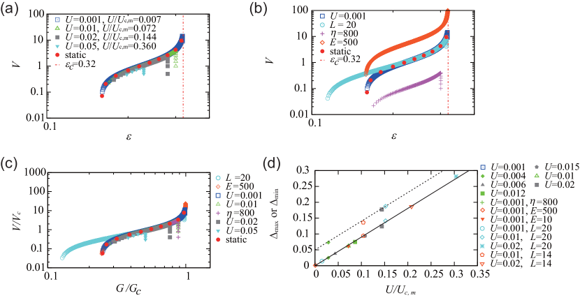
Figure 3: Results from the model with multi relaxation times. (a) $V$ vs $\varepsilon$ for different pulling speed $U$ for the fixed parameter set $(E,\eta,\varepsilon_{c},L,d)=(100,80,0.32,10,1)$, from which we obtain $U_{c,m}=0.139$. (b) $V$ vs $\varepsilon$ for the same pulling speed $U=0.001$ for different parameter sets. In the legends, the only parameter changed in the standard set given in the caption to (a) are given [except for the data labeled as $U=0.001$, which is the same data used in (a)]. (c) The data shown in (b) on renormalized axes $V/V_{c}$ and $G/G_{c}$. (d) Renormalized deviation of strains $\Delta_{\min}$ or $\Delta_{\max}$ defined in the text as a function of $U/U_{c,m}$. (For clarity, $\Delta_{\min}$ is shifted upwards by 0.05; the dashed and solid lines correspond to $\Delta_{\min}$ in Eq. (16) and $\Delta_{\max}$ in Eq. (15), respectively.) In the legends, the data for which only $U$ is shown are performed for the standard parameter set given in the caption to (a). The data for which $U$ and another parameter are given are performed for the standard set but with the parameter shown in the legend (except $U$) is replaced by the value.

Now, we confirm the above physical arguments by our numerical data obtained from simulation. In Fig. 3 (a), the relations between the crack-propagation speed $V$ and the global strain of the system $\varepsilon$ are given for the static and dynamic tests. The data are obtained for the same, standard parameter set $(E,\eta,\varepsilon_{c},L,d)=(100,80,0.32,10,1)$ as before so that differences reflect differences in the boundary conditions. As shown in the plot, we confirm that as the condition in Eq. (13) is less satisfied the least upper-bound strain $\varepsilon_{\max}$ and the greatest lower-bound strain $\varepsilon_{\min}$ for the $V-\varepsilon$ relation decreases and increases, respectively. (In the plot, $V$ looks scattered at $\varepsilon=\varepsilon_{\max}$; in fact, the highest $V$ value at $\varepsilon=\varepsilon_{\max}$, which is on the smooth curve suggested by the $V$ values at smaller epsilons, is the model prediction, while the other smaller $V$ values at $\varepsilon=\varepsilon_{\max}$ are added for guide for the eyes to recognize the position of $\varepsilon=\varepsilon_{\max}$.) In Fig. 3 (b) and (c), we show that the above results are not peculiar to the standard parameter set, and that the results obtained even at a velocity $U$ which does not satisfy Eq. (13) possess properties (A) and (B) but with $G_{\min}=E\varepsilon_{0}^{2}L/2$ and $G_{\max}=E\varepsilon_{c}^{2}L/2$, replaced by $G_{\min,c}$ and $G_{\max,c}$, respectively, with

$$G_{\min,c} =E\varepsilon_{\min}^{2}L/2$$ (17)

$$G_{\max,c} =E\varepsilon_{\max}^{2}L/2$$

Here, $\varepsilon_{\min}$ and $\varepsilon_{\max}$ satisfy Eqs. (16) and (15), respectively. In Fig. 3 (d), the relations given in Eqs. (15) and (16) are directly confirmed. These relations are quite natural as their simplest forms. This is because we generally expect that the dimensionless quantities on the left-hand sides that measure the deviations of the dynamic test from the static test, $\Delta_{\max}$ and $\Delta_{\min}$, should scale with the positive power of the dimensionless expression on the right-hand side $U/U_{c,m}$, which can naturally be constructed from the condition in Eq. (13). Note that the upwards shift of the $V-\varepsilon$ plot is not observed in the case of the model with multi relaxation times because the given stretching velocities $U$ are much smaller than those in the model with a single relaxation time.

III.3 Velocity jump in the static and dynamic tests

By employing the mechanism of velocity jump elucidated in the previous analytical theory sakumichi2017exactly , we can reproduce the velocity jump in our simple models in an ad hoc manner. The theory predicts that the glass transition that is very localized near the crack tip triggers the jump. Accordingly, to reproduce the velocity jump, we have only to vitrify the crack tip column by changing the elastic modulus of the springs in the column from $E$, corresponding to the rubbery modulus, to the glassy modulus $E_{G}$, if the strain exceeds the critical strain at the jump $\varepsilon_{J}$.

On the basis of the physical arguments we have developed above concerning the conditions for the static and dynamic tests to coincide with each other for the two simulation models, we expect that the positions just before and after the jump on the $V/V_{c}-G/G_{c}$ plot, characterized by the two points $(V_{b}$, $G_{J})$ and $(V_{a}$, $G_{J})$, are the same in the static and dynamic test if the condition in Eq. (6) or Eq. (13) is well satisfied.

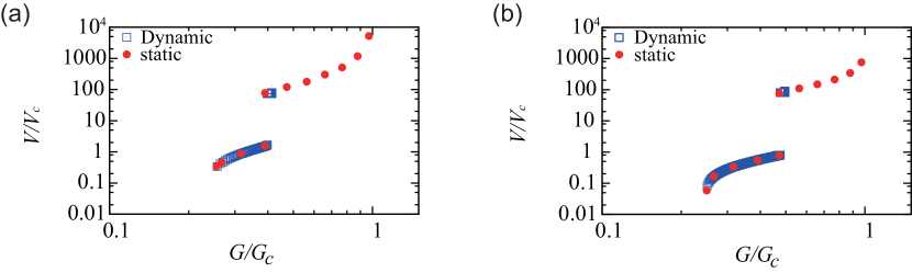
Figure 4: Comparison of the relation between $V/V_{c}$ and $G$ /$G_{c}$ in the static and dynamic tests obtained for the parameter set $(E,\eta,\varepsilon_{c},L,d)=(100,80,0.32,10,1)$. (a) Model with a single relaxation time where $U/U_{c}=0.008$. (b) Model with multi relaxation times where $U/U_{c,m}=0.007$.

This expectation is confirmed in Fig. 4, in which Eq. (6) and Eq. (13) are well satisfied for the models with a single relaxation time and multi relaxation times, respectively, in the dynamic test. As seen the figure, if Eq. (6) is well satisfied in the dynamic test for the model with a single relaxation time, the fracture energy $G_{J}=E\varepsilon_{J}^{2}L/2$ at the velocity jump, the velocities just before and after the transition $V_{b}$ and $V_{a}$ ($V_{b}<V_{a}$) are the exactly the same in the two tests (Here, we set $\varepsilon_{J}=0.2$ or $G_{J}/G_{c}=0.39$, and $E_{G}=100E$). The same is true for the model with multi relaxation times, if the condition given in Eq. (13) is satisfied (Here, we set $\varepsilon_{J}=0.22$ or $G_{J}/G_{c}=0.47$, and $E_{G}=100E$).

The range of the high velocity regime after the jump observed in the dynamic test is very narrow. This comes from the practical limitation for the width $W$ of the sample. If the width were long enough we would have the same range of the high velocity regime in the dynamic test, if Eq. (6) and Eq. (13) are well satisfied. After the jump, velocity increases significantly. Because of this, the crack tip soon reaches the opposite side edge of the sample in practice. The range of the low velocity regime before the jump could also become narrower (in the model with multi relaxation times) if $U$ is not small enough because the greatest lower bound increases according to Eq. (16).

In our previous work (see Fig. 5 and 6 of sakumichi2017exactly ), we showed that only the very vicinity of the crack tip is vitrified during stationary crack propagation at velocities above the velocity transition. This implies that the speed of vitrification is faster than any relaxation dynamics in the system, and that the strong tension transmitted from the boundary of vitrified region contributes to accelerate the crack propagation speed by expediting stress concentration around the crack tip to reach the critical strain $\varepsilon_{c}$. In this sense, our artificial manner of vitrification physically mimics the mechanism of accelerated crack propagation due to vitrification. In addition, it should be noted that in the static test the simulations at strains below and above vitrification are performed independently. Even in the dynamic test, the situation is essentially the same because we focus on a slow pulling-velocity regime, in which relaxation dynamics relevant for crack propagation is much faster than the time scale that characterizes the pulling speed. Note also that the energy release rate is defined based on homogeneous elastic energy developed well away from the crack tip and thus well defined in both cases of below and above transition.

IV Conclusion

In this study, we showed that the relation between the crack-propagation velocity $V$ and the strain $\varepsilon$ or the fracture energy (i.e., energy release rate) $G$ obtained from the static and dynamic tests are the same if the stretching velocity $U$ is smaller than a critical value, which we generally call $U_{CR}$ for later convenience. This is true even if the velocity jump exists. However, when the velocity jump is present, it is practically difficult to observe the full range of the high velocity regime after the jump because of the finite width of actual samples. (The small velocity regime also tends to be narrower if $U$ is not small enough.)

The present study provided the critical values $U_{CR}$ for the two simulation models [see Eqs. (6) and (13)] and their physical interpretation. On the basis of the interpretation, the critical value is universally given by the condition that the longest relaxation time of the sample is shorter than the time scale of stretching $L/U$ (because any practical system is the system with multi relaxation times). This condition could be hard to satisfy in practice for a system with long chains. However, this condition is relaxed if our purpose is limited to the detection of the velocity jump. This is because the jump positions just before and after jump, $(V_{b}$, $G_{J})$ and $(V_{a}$, $G_{J})$ with $G_{J}=E\varepsilon_{J}^{2}L/2$, are the same only if the strain at the jump $\varepsilon_{J}$ is in the range of the dynamic test, $\varepsilon_{\min}<\varepsilon<\varepsilon_{\max}$ , which is narrower than the range of the static test, $\varepsilon_{0}<\varepsilon<\varepsilon_{c}$.

The dynamic test is promising for the study of the velocity jump including non rubbery polymers because of the timesaving and cost-effective features and high sensitivity for detecting the velocity jump. Considering that the velocity jump has been utilized effectively for developing tough elastomers in the industry, the results of the present study are useful for developing tough polymers in general. This is especially because the previous study sakumichi2017exactly suggests theoretically that the velocity jump is expected be observed universally for variety of materials and the previous studies TomizawaJump2 and Takei2018 demonstrate experimentally that the dynamic test is more sensitive for detecting the velocity jump.

Appendix

.1 Details of the simulation models

In the lattice network, the four nearest neighbor cites of the cite $\mathbf{m}=(i,j)$ are specified by the indices $\mathbf{m}^{\prime}$ $=$ $(i-1,j),$ $(i,j+1),$ $(i+1,j),$ and $(i,j-1)$, which are called $\mathbf{m}_{s}$ with $s=1,$ 2, 3, and 4, respectively. The elongation vector $\Delta\mathbf{x}_{\mathbf{mm}^{\prime}}$ are defined as $\Delta\mathbf{x}_{\mathbf{mm}_{s}}=$ $\mathbf{x}_{\mathbf{m}}-\mathbf{x}_{\mathbf{m}_{s}}-\mathbf{d}_{s}$ with $\mathbf{d}_{1}=(d,0)=-\mathbf{d}_{3}$ and $\mathbf{d}_{4}=(0,d)=-\mathbf{d}_{2}$.

As mentioned in the text, in both of the two models in Eqs. (1) and (2), the dynamics of a bead is coupled with its nearest neighbors. For example, in the first case, the simulation algorithm is as follows. (i) We renew ”$\Delta\mathbf{x}_{\mathbf{m}}$ at the $i$-th step” on the basis of Eq. (1) to obtain ”the renewed $\Delta\mathbf{x}_{\mathbf{m}}$.” (ii) ”The renewed $\Delta\mathbf{x}_{\mathbf{m}}$ is transformed back to have ”$\mathbf{x}_{\mathbf{m}}$ at the $(i+1)$-th step.” (iii) From this ”$\mathbf{x}_{\mathbf{m}}$ at the $(i+1)$-th step”, we calculate ”$\Delta\mathbf{x}_{\mathbf{m}}$ at the $(i+1)$-th step” using Eq. (3). (iv) The ”$\Delta\mathbf{x}_{\mathbf{m}}$ at the $(i+1)$-th step” thus obtained is used for Eq. (1) to proceed to the $(i+2)$-th step. Note here the following: (A) Eq. (3) implies that $\Delta\mathbf{x}_{\mathbf{m}}$ is expressed as a linear combination of $\mathbf{x}_{\mathbf{m}}$ and thus are connected by a matrix. (B) ”The renewed $\Delta\mathbf{x}_{\mathbf{m}}$” and ”$\Delta\mathbf{x}_{\mathbf{m}}$ at the $(i+1)$-th step” in the above are generally different because of the coupling between $\mathbf{x}_{\mathbf{m}}$.

.2 Distribution of Relaxation times in the simulation models

To gain physical pictures of the models governed by Eqs. (4) and (5), we consider a creep test: we give a fixed stress $\sigma_{0}$ suddenly at time $t=0$ to observe the time development of the strain $\varepsilon(t)$ after $t=0$. In such a case, each column (in the $y$ direction) behaves in the same way as its neighbors and the shear force does not act at all: the problem reduces to one dimensional. For example, instead of Eq. (4), we have only to consider the equation

$$\gamma\frac{d}{dt}\Delta y_{\mathbf{m}}+k\Delta y_{\mathbf{m}} =Y_{\mathbf{m}}$$ (18)

$$\Delta y_{\mathbf{m}} =\Delta y_{\mathbf{mm}_{2}}+\Delta y_{\mathbf{mm}_{4}}$$ (19)

where $Y_{\mathbf{m}}=\sigma_{0}d^{2}$ for the beads at the top boundary and $Y_{\mathbf{m}}=0$ for the remaining bead. If we seek the elementary solution for Eq. (4) of the form $\Delta y_{\mathbf{m}}{=y}_{0}e^{-t/\tau}$, we find a single relaxation time $\tau=\gamma/k$. (The explicit solution for the creep test is given below.)

On the contrary, in Eq. (5), we find $N$ mutually-dependent equations

$$\gamma\frac{d}{dt}y_{\mathbf{mm}}+k\Delta y_{\mathbf{m}}=Y_{\mathbf{m}}$$ (20)

where $\Delta y_{\mathbf{m}}$ and $Y_{\mathbf{m}}$ are given as before. (The case of $N=1$ is special and is, in this specific case of the creep test, identified with the model with a single relaxation time for convenience.) This coupled equation set can be represented by a matrix formulation and the relaxation times can be obtained by solving an eigen-value problem of the matrix. By solving the eigen-value problem numerically, we obtained the distribution of relaxation times and examined explicitly a few selected characteristic relaxation times, the results of which are characterized in Fig. 5. The unit of time in the plots are set to $\tau_{0}=(5/16)\gamma/k$, where the smallest relaxation time $\tau_{\min}$ approaches this value as $N$ increases, as shown in (a). The largest and second largest relaxation times $\tau_{\max}$ and $\tau_{2nd}$ seem to scale as $N^{\nu}$ with the exponent $\nu$ close to $2$ as shown in (b). The lines in (b) represent the relations $\tau_{\max}/\tau_{0}=(2.49\pm 0.057)\times N^{1.89\pm 0.0006}$ and $\tau_{2nd}/\tau_{0}=(0.189\pm 0.008)\times N^{1.89\pm 0.0007}$, while we expect the exponent $\nu$ approaches 2 in the large $N$ limit on the basis of the physical interpretation we provided for Eq. (13).

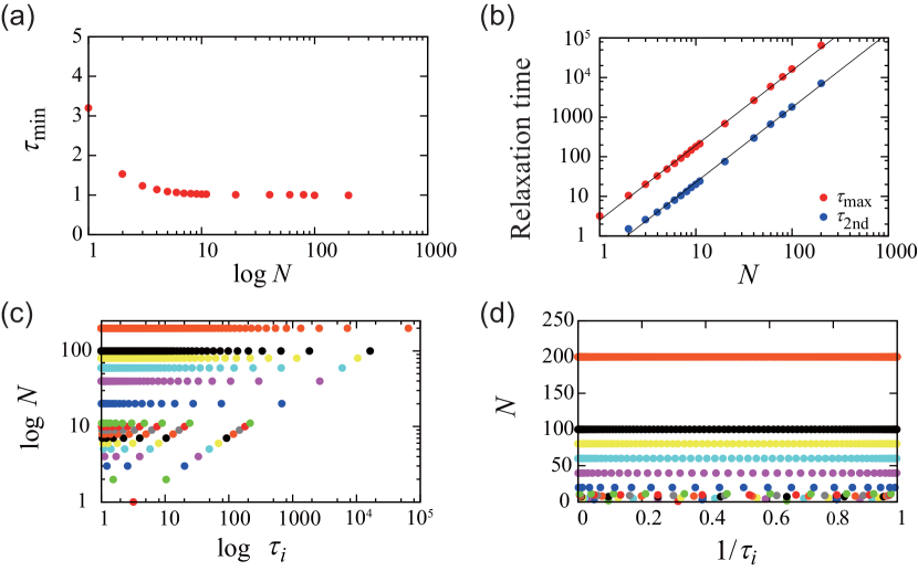
Figure 5: (a) The smallest relaxation time $\tau_{\min}$ vs $N$. (b) The largest and second largest relaxation times vs $N$. (c) Distribution of the relaxation time $\tau_{i}$ at different $N$, where each dot represents one mode. (d) Distribution of the inverse relaxation time $1/\tau_{i}$ at different different $N$. In the plots, the unit of time in the plots are set to $\tau_{0}=(5/16)\gamma/k$ with $\gamma/k=\eta/E$.

.3 Rheological properties of the simulation models

In this section, we demonstrate rheological properties of the two simulation models. For convenience, we first review and define rheological functions. The creep test is defined as follows: we give a fixed stress $\sigma_{0}$ suddenly at time $t=0$ to observe the time development of the strain $\varepsilon(t)$ after $t=0$. From $\varepsilon(t)$ thus obtained, the extensional creep compliance $D(t)$ is given as

$$\varepsilon(t)=D(t)\sigma_{0}$$ (21)

The complex compliance $D^{\ast}(\omega)$ is introduced by the following equation:

$$D^{\ast}(\omega)=i\omega\int_{0}^{\infty}D(t)e^{-i\omega t}dt$$ (22)

This quantity and the complex modulus $E(\omega)$ satisfies the following equation ferry1980viscoelastic :

$$E^{\ast}(\omega)=\frac{1}{D^{\ast}(\omega)}=E^{\prime}(\omega)-iE^{\prime\prime}(\omega)$$ (23)

By using Eqs. (21) to (23), we can obtain rheological functions $D(t)$, $E^{\prime}(\omega)$, and $E^{\prime\prime}(\omega)$ from the function $\varepsilon(t)$ obtained from the creep test.

.3.1 Model with a single relaxation time

On the basis of the equation of motion for the creep test in this model, given in Eq. (18), we obtain $\varepsilon(t)=(\sigma_{0}/E)(1-e^{-t/\tau})$ with $\tau=\gamma/k=\eta/E$. Thus, from Eq. (21), the creep compliance is given by

$$D(t)=\frac{1}{E}\left(1-e^{-\frac{E}{\eta}t}\right)$$ (24)

From Eq. (22), we obtain $D(\omega)$ as

$$D(\omega)=\frac{\omega}{E\omega+i\eta\omega^{2}}$$ (25)

by assuming that $\omega$ has an infinitely-small negative imaginary part for the integral to converge. From this expression, we obtain $E(\omega)$ from Eq. (23):

$$E(\omega)=\frac{E\omega+i\eta\omega^{2}}{\omega}$$ (26)

From this, we obtain

$$E^{\prime}(\omega)=E$$ (27)

$$E^{\prime\prime}(\omega)=\eta\omega$$ (28)

.3.2 Model with multi relaxation times

For this model, we first obtain the function $\varepsilon(t)$ numerically for the parameter set $(\eta,E)=(80,100)$, and fit the function with an analytical expression in the following form with regarding $\tau_{n}$ as fitting parameters and selecting $a$ for a given stress for the creep test:

$$a\sum_{n}(1-e^{-t/\tau_{n}})$$ (29)

On the basis of the analytical expression, we demonstrate plots of $D(\omega)$, $E^{\prime}(\omega)$, and $E^{\prime\prime}(\omega)$ in Figs. 6 and 7 below. For $N\leq 12$, we used a sum of $N$ functions for the fitting for simplicity ($a$ is set to 0.01 for a given stress $\sigma_{0}=20$, corresponding to a saturation value of the strain at long times, $\sigma_{0}/E=$ $0.2$). However, for $N>12$, we used a sum of only 12 functions for convenience: our results below is subject to errors to a certain degree. More complete examination will be discussed elsewhere.

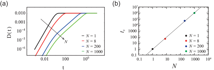
Figure 6: (a) Creep compliance $D(t)$ for different $N$. (b) The saturation time $t_{S}$ as a function $N$. In the plots, the unit of time is $\eta/E$ with $\eta=80$ and $E=100$.

In Fig. 6, we show the creep compliance $D(t)$ numerically obtained based on Eq. (20). This function approaches the saturation value $1/E=1/100$ at the saturation time $t_{S}$. This time is defined as the time at the intersection of two extrapolations lines, one from the saturated plateau region and the other from the region of straight line with positive slope next to the plateau region. The time $t_{S}$ is given as a function of $N$ in (b), in which the data are fitted by $t_{S}=c_{S}N^{\nu_{S}}$ with $c_{S}=2.6\pm 0.01$ and $\nu_{S}=1.86\pm 0.00065$. Comparing this numerical fitting with the one we obtained for $\tau_{\max}$ given in the previous section, $t_{S}$ can physically be identified with $\tau_{\max}$, which implies that the rheological functions are characterized by the longest relaxation time $\tau_{\max}$.

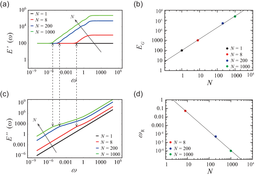
Figure 7: (a) $E^{\prime}(\omega)$ for different $N$. (b) Glass modulus $E_{G}$ ($E^{\prime}(\omega)$ for large $\omega$) as a function of $N$. (c) $E^{\prime\prime}(\omega)$ for different $N$. (d) Rubber frequency $\omega_{R}$ ($\omega$ at which the initial rubbery plateau terminates) as a function of $N$. In the plots, the unit of time is $\eta/E$ with $\eta=80$ and $E=100$, as before.

In Fig. 7 (a), we show numerically obtained complex modulus $E(\omega)$ for the model with multi relaxation times at different $N$. In (a), we confirm that our model possesses the rubbery plateau $(E=100)$ on the low frequency side and the glassy plateau on the high frequency side. The glassy modulus $E_{G}$ increases with $N$, which is quantified in (b). The data is fitted by $E_{G}=c_{G}N^{\nu_{G}}$ with $c_{G}=99.62\pm 0.017$ and $\nu_{G}=1.14\pm 0.008$. The initial rubbery plateau is terminated at $\omega=\omega_{R}$, at which $E^{\prime\prime}(\omega)$ starts to deviate from the initial straight line as seen in (c). The rubbery frequency $\omega_{R}$ decreases with $N$, which is quantified in (d). The data is fitted by $\omega_{R}=c_{R}N^{\nu_{R}}$ with $c_{R}=5.48\pm 0.032$ and $\nu_{R}=-2.23\pm 0.0036$. The characteristic time $1/\omega_{R}$ may be identified with $\tau_{\max}$, which again suggests that the rheological functions are characterized by the longest relaxation time $\tau_{\max}$.

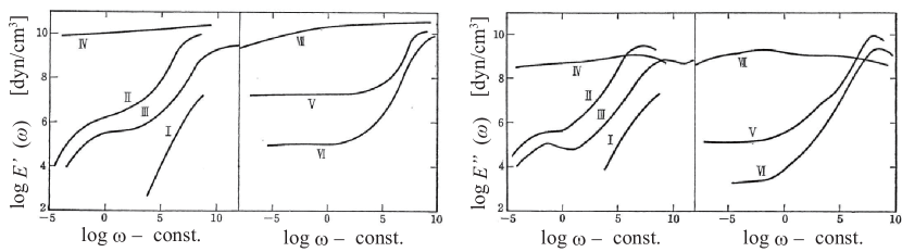
Figure 8: Typical plots of $E^{\prime}(\omega)$ and $E^{\prime\prime}(\omega)$ obtained from polymers introduced in the classic text ferry1980viscoelastic .

For completeness, we show in Fig. 8 typical rheology data for various polymers. By comparing these plots and plots in Fig. 7(a) and (c), we see that our model with multi relaxation times is capable of describing essential features of polymer rheologies.