Brownian motion with alternately fluctuating diffusivity:
Stretched-exponential and power-law relaxation

Abstract

We investigate Brownian motion with diffusivity alternately fluctuating between fast and slow states. We assume that sojourn-time distributions of these two states are given by exponential or power-law distributions. We develop a theory of alternating renewal processes to study a relaxation function which is expressed with an integral of the diffusivity over time. This relaxation function can be related to a position correlation function if the particle is in a harmonic potential, and to the self-intermediate scattering function if the potential force is absent. It is theoretically shown that, at short times, the exponential relaxation or the stretched-exponential relaxation are observed depending on the power law index of the sojourn-time distributions. In contrast, at long times, a power law decay with an exponential cutoff is observed. The dependencies on the initial ensembles (i.e., equilibrium or non-equilibrium initial ensembles) are also elucidated. These theoretical results are consistent with numerical simulations.

I Introduction

The Brownian motion, which is random motion of microscopic particles suspended in fluids, is observed in various systems. The examples are colloid dynamics in suspensions Dhont (1996), beads and center-of-mass motion of polymer chains Doi and Edwards (1986), and macromolecular diffusion in intracellular environments Bressloff and Newby (2013). The Brownian motion is usually characterized by mean square displacements (MSDs). In fact, the MSD for a simple Brownian particle increases linearly with time, and the proportionality factor is the diffusion coefficient multiplied by $2d$ with $d$ being the spatial dimension of the system in which the Brownian particle is immersed. The diffusion coefficient of a rigid particle depends on its shape and the viscosity of the surrounding fluid Landau and Lifshitz (1987); Kim and Karrila (2013). For example, the diffusion coefficient of a spherical particle with a small Reynolds number is given by the Stokes law, $D=k_{B}T/6\pi\eta a$, with $k_{B}$ the Boltzmann constant, $T$ the absolute temperature, $\eta$ the viscosity of the fluids, and $a$ the radius of the particle.

The diffusion coefficient is usually considered as constant and is independent of time. However, this is not always true; in crowded systems such as supercooled liquids Yamamoto and Onuki (1998a, b) and intracellular environments Parry et al. (2014), the diffusion coefficient is not a constant, and often behaves like a random variable. For such systems, the diffusion coefficient should be interpreted as a time-dependent and fluctuating quantity. The center-of-mass motion of polymer chains actually exhibits time-dependent and fluctuating diffusivity Uneyama et al. (2012, 2015); Miyaguchi (2017). A prominent feature of such Brownian motion with fluctuating diffusivity is that its displacement distribution becomes non-Gaussian, though the MSD shows normal diffusion (i.e., the linear time dependence of the MSD mentioned above) Chubynsky and Slater (2014); Uneyama et al. (2015).

Recently, Brownian motion with fluctuating diffusivity has been intensively studied in the absence of the external force Chubynsky and Slater (2014); Uneyama et al. (2015); Manzo et al. (2015); Chechkin et al. (2017); Miyaguchi (2017); Jain and Sebastian (2017), but it would be also important to investigate the Brownian dynamics with some external forces, such as the forces by some confinements and external potentials. For example, the diffusion coefficient observed in single-particle-tracking experiments in bacterial cytoplasms is typically of the order of $10^{-2}\,[\text{\textmu}\mathrm{m}^{2}/\mathrm{sec}]$ Golding and Cox (2006); Parry et al. (2014), whereas the size of the bacterial cell is of the order of $1\text{\textmu}\mathrm{m}$. Thus, the time for diffusion across a cell is of the order of $10\,\mathrm{sec}$ Milo and Phillips (2015). On the other hand, the measurement times of single-particle-tracking experiments are often longer than $10\,\mathrm{sec}$ Golding and Cox (2006); Parry et al. (2014), and thus effects of confinement inside the cells cannot be ignored.

In Ref. Uneyama et al. (2019), the authors analyzed the Brownian particle with fluctuating diffusivity confined in a harmonic potential, that is, the Ornstein-Uhlenbeck process with fluctuating diffusivity (OUFD). In particular, a relaxation function $\Phi(t)$ of the position coordinates [See Eq. (5) below] was studied instead of the MSD [the MSD is easily derived from $\Phi(t)$, if the system is in equilibrium]. In Ref. Uneyama et al. (2019), the diffusion coefficient $D(t)$ is assumed to be Markovian stochastic processes, and an eigenmode expansion for the relaxation function $\Phi(t)$ is obtained through the eigenmode analysis of a transfer operator. Formally, these results can be applicable to any systems with the Markovian diffusivity $D(t)$. But it is also important to study systems with non-Markovian diffusivity $D(t)$, because some properties (such as a large scatter of a time-averaged MSD and weak ergodicity breaking) observed in single-particle-tracking experiments Golding and Cox (2006); Weber et al. (2010); Weigel et al. (2011); Jeon et al. (2011); Burov et al. (2011); Tabei et al. (2013); Yamamoto et al. (2014) are believed to originate from non-Markovian properties of the system He et al. (2008); Meroz et al. (2010); Jeon et al. (2011); Burov et al. (2011); Tabei et al. (2013); Miyaguchi and Akimoto (2011).

In this paper, we study the Brownian motion with $D(t)$ being a non-Markovian stochastic process. Because general analysis for the non-Markovian diffusivity $D(t)$ is extremely difficult, we assume that $D(t)$ takes only two values $D_{+}$ and $D_{-}$, and randomly switches between these two states (the fast and slow states). It would be worth noting that such two-state diffusion dynamics is actually a good approximation to describe protein diffusion along DNA strands Leith et al. (2012), large colloidal diffusion in bacterial cytoplasm Parry et al. (2014), and movement patterns of several kinds of bacteria Detcheverry (2017). To theoretically analyze such two-state dynamics, we use the alternating renewal theory Cox (1962); Goychuk and Hänggi (2003); Akimoto and Seki (2015); Miyaguchi et al. (2016), in which the system is assumed to switch randomly between the two states. Similar theoretical framework for the two-state dynamics is developed by utilizing non-commutable operator calculus in Ref. Detcheverry (2017).

Furthermore, sojourn-time distributions for the two states are assumed to be a power law in this paper, which is a typical non-Markovian stochastic process. As discussed in Ref. Miyaguchi et al. (2016), such power-law sojourn-time distributions can originate from the cage effects in crowded systems Odagaki and Hiwatari (1990); Doliwa and Heuer (2003); Helfferich et al. (2014) or spatial heterogeneity. Due to the power-law sojourn-time distribution, the relaxation function $\Phi(t)$ shows exponential or stretched-exponential decay at short times, whereas power-law decay with an exponential cutoff at long times.

This paper is organized as follows. In Sec. II, the OUFD and the Langevin equation with fluctuating diffusivity (LEFD) are defined. In Sec. II, the sojourn-time distribution and the initial ensembles are also introduced. In Sec. III, by utilizing an alternating renewal theory, the relaxation function is represented with the sojourn-time distributions. In Sec. IV, the relaxation function is derived for the exponential and the power-law sojourn-time distributions. Finally, Sec. V is devoted to a discussion. In Appendices, we summarize some technical matters, including simulation details.

II Definition of the models

In this section, we define the OUFD, and introduce a position correlation function $\Phi(t)$. In addition, the LEFD is also introduced, and it is shown that the self-intermediate scattering function is given by a formula similar to $\Phi(t)$.

II.1 Ornstein-Uhlenbeck process with fluctuating diffusivity

The Ornstein-Uhlenbeck process with fluctuating diffusivity is defined by the following equation Uneyama et al. (2015, 2019):

$$\frac{d\bm{r}(t)}{dt}=-\frac{\tilde{u}\bm{r}(t)}{\gamma(t)}+\sqrt{2D(t)}\bm{\xi}(t),$$ (1)

where $\bm{r}(t)$ is the $d$-dimensional position vector of the Brownian particle at time $t$, $\gamma(t)$ is a friction coefficient, and $\tilde{u}$ is a constant which characterizes the strength of the restoring force [$\tilde{u}$ can be related to the spring constant of a harmonic potential $U(\bm{r})$, as $U(\bm{r})=\tilde{u}\bm{r}^{2}/2$].

The diffusion coefficient $D(t)$ is time dependent and fluctuating, i.e., $D(t)$ is a stochastic process. Moreover, $\bm{\xi}(t)$ is a white Gaussian noise which satisfies

$$\left\langle\bm{\xi}(t)\right\rangle_{\bm{\xi}}=0,\qquad\left\langle\bm{\xi}(t)\bm{\xi}(t^{\prime})\right\rangle_{\bm{\xi}}=\bm{I}\delta(t-t^{\prime}),$$ (2)

where $\bm{I}$ is the identity matrix, and we use the notation $\left\langle\dots\right\rangle_{\bm{\xi}}$ to represent an ensemble average over the noise history $\bm{\xi}(t)$. It is also assumed that $\bm{\xi}(t)$ and $D(t)$ are mutually independent.

Because of Eq. (2), the thermal noise is delta-correlated as

$$\left\langle\sqrt{D(t)}\bm{\xi}(t)\sqrt{D(t^{\prime})}\bm{\xi}(t^{\prime})\right\rangle_{\bm{\xi}}=D(t)\bm{I}\delta(t-t^{\prime}).$$ (3)

We require that the system can reach the equilibrium state if the process $D(t)$ can reach the equilibrium state. This is equivalent to require that the detailed-balance condition (or the local equilibrium condition) is satisfied for the friction and noise coefficients Sekimoto (2010).

$$\frac{k_{B}T}{\gamma(t)}=D(t).$$ (4)

Multiplying both sides of Eq. (1) by $\bm{r}(0)$, and averaging over a noise history $\bm{\xi}(t)$, we have an ordinary differential equation $d\left\langle\bm{r}(t)\cdot\bm{r}(0)\right\rangle_{\bm{\xi}}/dt=-uD(t)\left\langle\bm{r}(t)\cdot\bm{r}(0)\right\rangle_{\bm{\xi}}$, where we define $u$ as $u:=\tilde{u}/k_{B}T$ and used $\left\langle\bm{\xi}(t)\cdot\bm{r}(0)\right\rangle_{\bm{\xi}}=0$. Integrating this equation and averaging over realizations of $D(t)$ as well as initial distributions of $\bm{r}(0)$, we have a relaxation function

$$\Phi(t):=\frac{\left\langle\bm{r}(t)\cdot\bm{r}(0)\right\rangle_{\bm{\xi},\mathrm{I},D}}{\left\langle\bm{r}^{2}(0)\right\rangle_{\mathrm{I}}}=\left\langle\exp\left[-u\int_{0}^{t}dt^{\prime}D(t^{\prime})\right]\right\rangle_{D},$$ (5)

where the subscripts $D$ and $\mathrm{I}$ represent the ensemble averages over $D(t)$ and $\bm{r}(0)$, respectively.

It follows from Eq. (5) that the relaxation function $\Phi(t)$ is independent of the initial distributions of $\bm{r}(0)$; namely, $\Phi(t)$ is characterized only by the stochastic process $D(t)$. In numerical simulations, we use the local equilibrium distribution $(u/2\pi)^{d/2}\exp\left[-u\bm{r}^{2}(0)/2\right]$ as an initial distribution of $\bm{r}(0)$, but the results are independent of the choice of the initial distribution. Therefore, whether $\bm{r}(0)$ follows the local equilibrium distribution or not is unimportant concerning the relaxation function $\Phi(t)$. From Eq. (5), on the other hand, the relaxation function clearly depends on $D(t)$ and thus the statistical properties of the stochastic process $D(t)$ is important. In this work, we consider rather general stochastic processes for $D(t)$ including the one that may not reach the equilibrium state (See Sec. IV.3). We use the words equilibrium and non-equilibrium to specify the initial ensembles of the stochastic process $D(t)$. We will explain these initial ensembles in Sec. II.3 and Appendix A.

Moreover, if the system is in a stationary state—i.e., if $\bm{r}(0)$ follows the local equilibrium distribution and $D(t)$ is a stationary stochastic process—the MSD is given by Uneyama et al. (2019)

$$\left\langle|\bm{r}(t)-\bm{r}(0)|^{2}\right\rangle_{\bm{\xi},\mathrm{I},D}=2\left\langle\bm{r}^{2}(0)\right\rangle_{\mathrm{I}}\left[1-\Phi(t)\right].$$ (6)

Thus, the MSD is easily obtained from the relaxation function $\Phi(t)$, if the system is stationary.

II.2 Langevin equation with fluctuating diffusivity

In this subsection, we show that the relaxation function $\Phi(t)$ given by Eq. (5) is related to the self-intermediate scattering function for the LEFD

$$\frac{d\bm{r}(t)}{dt}=\sqrt{2D(t)}\bm{\xi}(t),$$ (7)

where the potential term is absent, and thus it is translationally invariant in space. To study dynamical behavior of such a system, a density correlation function $\left\langle\delta(\bm{r}^{\prime\prime}-\bm{r}(t^{\prime\prime}))\delta(\bm{r}^{\prime}-\bm{r}(t^{\prime}))\right\rangle_{\bm{\xi},D}$ is convenient. Due to the translational symmetry, this correlation function depends on the position coordinates $\bm{r}^{\prime\prime}$ and $\bm{r}^{\prime}$ only through the displacement $\bm{r}:=\bm{r}^{\prime\prime}-\bm{r}^{\prime}$. By also using a lag time $t:=t^{\prime\prime}-t^{\prime}$, the correlation function is rewritten as $\left\langle\delta(\bm{r}+\bm{r}^{\prime}-\bm{r}(t+t^{\prime}))\delta(\bm{r}^{\prime}-\bm{r}(t^{\prime}))\right\rangle_{\bm{\xi},D}$. Integrating with $\bm{r}^{\prime}$, we obtain Hansen and McDonald (1990)

$$G_{s}(\bm{r},t):=\left\langle\delta\left(\bm{r}-\left[\bm{r}(t)-\bm{r}(0)\right]\right)\right\rangle_{\bm{\xi},\mathrm{I},D},$$ (8)

where we set $t^{\prime}=0$ and take the average over $\bm{r}(0)$. Note that $D(t)$ is not stationary in general, thus $G_{s}(\bm{r},t)$ depends on the choice of the origin of time. This distribution function for the particle displacement $G_{s}(\bm{r},t)$ is called the van Hove self-correlation function and it is widely utilized to study the dynamical behavior of glass formers [From the spherical symmetry, the angular integration of $G_{s}(\bm{r},t)$ gives $4\pi r^{2}G_{s}(r,t)$ with $r=|\bm{r}|$, and this latter function is usually utilized Kob and Andersen (1995)].

Here, let us consider the same quantity with a given $D(t)$.

$$G_{s}[\bm{r},t|D]:=\left\langle\delta\left(\bm{r}-\left[\bm{r}(t)-\bm{r}(0)\right]\right)\right\rangle_{\bm{\xi},\mathrm{I}},$$ (9)

where the ensemble average for $D(t)$ is not taken.

Note that this correlation function is a functional of $D(t)$ and is related to $G_{s}(\bm{r},t)$ by

$$G_{s}(\bm{r},t)=\left\langle G_{s}\!\left[\bm{r},t|D\right]\right\rangle_{D}=\int\mathcal{D}\!D\,G_{s}\!\left[\bm{r},t|D\right]\,\mathcal{P}\!\left[\mathcal{D}\right],$$ (10)

where $\int\mathcal{D}\!D$ represents the path integral (functional integral) over the diffusivity $D(t)$ and $\mathcal{P}[\mathcal{D}]$ is a path probability of $D(t)$.

The functional $G_{s}[\bm{r},t|D]$ is equivalent to a propagator of the Brownian particle for a given $D(t)$, and thus it follows the Fokker-Planck equation Berne and Pecora (2000)

$$\frac{\partial G_{s}[\bm{r},t|D]}{\partial t}=D(t)\nabla^{2}G_{s}[\bm{r},t|D],$$ (11)

with an initial condition $G_{s}[\bm{r},0|D]=\delta(\bm{r})$. Here, $\nabla^{2}$ is the Laplacian operator. This Fokker-Planck equation is solved by using a Fourier transform

$$F_{s}[\bm{k},t|D]:=\int d\bm{r}e^{-i\bm{k}\cdot\bm{r}}G_{s}[\bm{r},t|D].$$ (12)

This functional is related to the self-intermediate scattering function as shown below. The Fourier transform of Eq. (11) is given by

$$\frac{\partial F_{s}[\bm{k},t|D]}{\partial t}=-D(t)k^{2}F_{s}[\bm{k},t|D],$$ (13)

with an initial condition $F_{s}[\bm{k},0|D]=1$ and $k=|\bm{k}|$. This differential equation is easily solved, and we obtain

$$F_{s}[\bm{k},t|D]=\exp\left[-k^{2}\int_{0}^{t}D(t^{\prime})dt^{\prime}\right].$$ (14)

The Fourier transform $F_{s}(\bm{k},t)$ of the correlation function $G_{s}(\bm{r},t)$ is usually referred to as the self-intermediate scattering function and widely utilized to study dynamical behavior of glass formers. By using Eq. (14), the function $F_{s}(\bm{k},t)$ is given by

$$F_{s}(\bm{k},t)=\left\langle\exp\left[-k^{2}\int_{0}^{t}D(t^{\prime})dt^{\prime}\right]\right\rangle_{D}.$$ (15)

Note that this function $F_{s}(\bm{k},t)$ has the same form as $\Phi(t)$ in Eq. (5). A similar result was also derived in Ref. Jain and Sebastian (2017) in a slightly different way.

II.3 Definition of initial ensemble

In this subsection, the stochastic process $D(t)$ is defined as a two-state process, and sojourn-time distributions for these states are introduced. If the stochastic process $D(t)$ is a Markovian process, the system can reach the equilibrium state if the detailed blance is satisfied (for the Markovian processes, whether the detailed blance is satisfied or not can be checked rather straightforwardly). On the other hand, in this work, we consider more general processes for $D(t)$ which can be non-Markovian. Thus the situation is (at least apparently) not intuitive. Here we briefly explain the defintions of equilibrium and non-equilibrium initial states. The detailed derivations for them are presented in Appendix A.

In this paper, the diffusion coefficient $D(t)$ is assumed to be a dichotomous process as illustrated in Fig. 1. Namely, at each time $t$, the value of $D(t)$ is either of the two values $D_{+}$ or $D_{-}$:

$$D(t):=\begin{cases}D_{+}\quad(+\,\text{state; fast state}),\\[2.84544pt] D_{-}\quad(-\,\text{state; slow sate}).\end{cases}$$ (16)

In addition, we assume that $0\leq D_{-}<D_{+}$. The condition $D_{-}\geq 0$ is used for calculating double unilateral Laplace transforms in Eq. (25) below. Contrastingly, in Ref. Godrèche and Luck (2001), a similar calculation is carried out by using a bilateral Laplace transform, thereby obtaining an equation corresponding to Eq. (25). This difference in computation originates from the fact that, in Ref. Godrèche and Luck (2001), a value corresponding to $D_{-}$ is set as $-1$ (In Ref. Godrèche and Luck (2001), this corresponding variable is not the diffusion coefficient, but it is related to the position of a diffusing particle. Thus, the negative value is physically relevant).

We define the dichotomous process $D(t)$ by using the times at which the transitions between the two states occur, $t_{n}\,(n=1,2,\dots)$; these times are referred to as renewal times [we also set $t_{0}=0$ for convenience, though $t_{0}$ is not a renewal time in general. See Fig. 1(a)]. The renewal time $t_{n}\,(n=1,2,\dots)$ can be written by a sum of successive sojourn times in the two states, $\tau_{k}$ ($k=1,2,\dots$), as $t_{n}\equiv\sum_{k=1}^{n}\tau_{k}$. A switching rule between the two states can then be given by sojourn-time probability density functions (PDFs) of these states. Namely, the sojourn times $\tau_{k}\,(k=2,3,\dots)$ for $+$ and $-$ states are random variables that follow sojourn-time PDFs, $\rho^{+}(\tau)$ and $\rho^{-}(\tau)$, respectively.

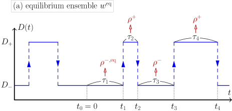
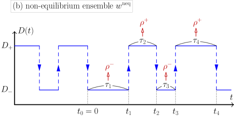
Figure 1: (Color online) Schematic illustration of the switching process of diffusivity $D(t)$. (a) For the equilibrium ensemble $w^{\mathrm{eq}}(\tau_{1})$, the process starts at $t=-\infty$, and thus there is no transition at $t=t_{0}$ in general. As an example, a realization with $D(0)=D_{-}$ is shown; For this trajectory, $\tau_{2n}\,(n=1,2,\dots)$ follow the sojourn-time PDF $\rho^{+}(\tau)$, whereas $\tau_{2n+1}\,(n=1,2,\dots)$ follow $\rho^{-}(\tau)$. The first sojourn time $\tau_{1}$, however, follows the equilibrium PDF $\rho^{-,\mathrm{eq}}(\tau)$. (b) For the non-equilibrium ensemble $w^{\mathrm{neq}}(\tau_{1})$, it is assumed that a transition occurs at $t=t_{0}$. As an example, a realization with $D(0)=D_{-}$ is shown; For this trajectory, $\tau_{2n}\,(n=1,2,\dots)$ follow the sojourn-time PDF $\rho^{+}(\tau)$, whereas $\tau_{2n+1}\,(n=0,1,\dots)$ follow $\rho^{-}(\tau)$.

To fully specify the process $D(t)$, we also need to define the PDF for the first sojourn time $\tau_{1}$ (See Fig. 1). We mainly study two kinds of the first sojourn-time PDFs: the equilibrium and non-equilibrium ensembles.

II.3.1 Equilibrium ensemble

For the equilibrium ensemble, the process starts at $t=-\infty$, and thus the system is in equilibrium at $t=0$. The diffusivity $D(0)$ is therefore at $+$ or $-$ state with equilibrium fractions $p_{+}^{\mathrm{eq}}$ and $p_{-}^{\mathrm{eq}}$. These fractions $p_{\pm}^{\mathrm{eq}}$ are simply given by

$$p_{\pm}^{\mathrm{eq}}=\frac{\mu_{\pm}}{\mu_{+}+\mu_{-}},$$ (17)

where $\mu_{\pm}$ are mean sojourn times for $\rho^{\pm}(\tau)$. From this expression, it is clear that the equilibrium ensemble exists only when the mean sojourn times $\mu_{\pm}$ are finite; if $\mu_{\pm}$ diverges, the system cannot reach the equilibrium state Miyaguchi and Akimoto (2013).

Moreover, the first sojourn time $\tau_{1}$ follows an equilibrium sojourn-time PDF $\rho^{\pm,\mathrm{eq}}(\tau_{1})$, not $\rho^{\pm}(\tau_{1})$. This is because, in the equilibrium ensemble, $t=0$ is not a renewal time as illustrated in Fig. 1(a). Thus, the PDF of $\tau_{1}$ in the equilibrium ensemble is given by

$$w^{\mathrm{eq}}_{+}(\tau_{1})+w^{\mathrm{eq}}_{-}(\tau_{1})=p_{+}^{\mathrm{eq}}\rho^{+,\mathrm{eq}}(\tau_{1})+p_{-}^{\mathrm{eq}}\rho^{-,\mathrm{eq}}(\tau_{1}),$$ (18)

where $w^{\mathrm{eq}}_{\pm}(\tau_{1})$ is defined by $w^{\mathrm{eq}}_{\pm}(\tau_{1}):=p_{\pm}^{\mathrm{eq}}\rho^{\pm,\mathrm{eq}}(\tau_{1})$. Namely, $\rho^{\pm,eq}(\tau_{1})$ is a conditional PDF of the first sojourn time $\tau_{1}$ given that the process starts at $t=-\infty$ and the state is $\pm$ at $t=0$. For a derivation and an explicit expression of $\rho^{\pm,\mathrm{eq}}(\tau)$, see Appendix A.

II.3.2 Non-equilibrium ensemble

We also study a non-equilibrium ensemble. Here, we limit ourselves that a transition occurs exactly at the inital time $t=0$ [See Fig. 1(b)], and call such an ensemble as non-equilibrium. Note that this is a typical non-equilibrium ensemble employed in the renewal theory Godrèche and Luck (2001) and CTRW theory Miyaguchi and Akimoto (2013). In this ensemble, the diffusivity $D(0)$ is at $+$ or $-$ state with some inital fractions $p_{+}^{0}$ and $p_{-}^{0}$; one of these fractions is arbitrary, and the other is given by the normalization $p_{+}^{0}+p_{-}^{0}=1$.

Moreover, if $D(0)=D_{\pm}$, the first sojourn time $\tau_{1}$ follows the sojourn-time PDF $\rho^{\pm}(\tau_{1})$; i.e., the first sojourn-time PDF is the same as those for the following sojourn times $\tau_{n}\,(n=3,5,\dots)$. This is because we assume that $t=0$ is a renewal time for the non-equilibrium ensemble. It follows that, the first sojourn-time PDF is given by

$$w^{\mathrm{neq}}_{+}(\tau_{1})+w^{\mathrm{neq}}_{-}(\tau_{1})=p_{+}^{0}\rho^{+}(\tau_{1})+p_{-}^{0}\rho^{-}(\tau_{1}),$$ (19)

where $w^{\mathrm{neq}}_{\pm}(\tau_{1})$ is defined by $w^{\mathrm{neq}}_{\pm}(\tau_{1}):=p_{\pm}^{0}\rho^{\pm}(\tau_{1})$.

II.3.3 General ensemble

In the next section, we present a theory for a more general inital ensemble rather than the specific ensembles defined above. Let us denote this general inital ensemble as

$$w^{0}_{+}(\tau_{1})+w^{0}_{-}(\tau_{1})=p_{+}^{0}\rho^{+,0}(\tau_{1})+p_{-}^{0}\rho^{-,0}(\tau_{1}),$$ (20)

where $w^{0}_{\pm}(\tau_{1}):=p_{\pm}^{0}\rho^{\pm,0}(\tau_{1})$, and $\rho^{\pm,0}(\tau)$ is the first sojourn-time PDF given that the initial state is $\pm$. Therefore, if we replace $p_{\pm}^{0}$ and $\rho^{\pm,0}(\tau_{1})$ in Eq. (20) with $p_{\pm}^{\mathrm{eq}}$ and $\rho^{\pm,\mathrm{eq}}(\tau_{1})$, we obtain the equilibrium ensemble defined in Eq. (18); similarly, if we replace $\rho^{\pm,0}(\tau_{1})$ in Eq. (20) with $\rho^{\pm}(\tau_{1})$, we obtain the non-equilibrium ensemble defined in Eq. (19). These replacement rules are used in the following sections to obtain results for the equilibrium and non-equilibrium ensembles.

We also use notations such as $w^{0}(\tau_{1}):=w_{+}^{0}(\tau_{1})+w_{-}^{0}(\tau_{1})$, $w^{\mathrm{eq}}(\tau_{1}):=w_{+}^{\mathrm{eq}}(\tau_{1})+w_{-}^{\mathrm{eq}}(\tau_{1})$ and $w^{\mathrm{neq}}(\tau_{1}):=w_{+}^{\mathrm{neq}}(\tau_{1})+w_{-}^{\mathrm{neq}}(\tau_{1})$, with which we can completely specify the initial ensemble for $D(t)$. Moreover, instead of the notation $\left\langle\dots\right\rangle_{D}$ used in the previous subsections, hereafter we employ the following notations for the ensemble average over $D(t)$. We denote the average in terms of the equilibrium ensembles $w^{\mathrm{eq}}(\tau_{1})$ as $\left\langle\dots\right\rangle_{\mathrm{eq}}$, and the average in terms of the genelal initial ensemble $w^{0}(\tau_{1})$ as $\left\langle\dots\right\rangle$ (the bracket without a subscript).

III Alternating renewal theory: general analysis

In this section, we derive a general formula for the relaxation function $\Phi(t)$ by using the alternating renewal theory Cox (1962); Miyaguchi et al. (2016), in which the system has two states with different sojourn-time PDFs in general. In fact, we show that $\Phi(t)$ is closely related to a quantity which is called occupation times in the renewal theory Godrèche and Luck (2001).

III.1 Definition of occupation time

To explicitly represent the variables and initial conditions, let us denote the relaxation function $\Phi(t)$ as $\hat{f}^{D}(u;t|w^{0})$; namely [see Eq. (5)]

$$\hat{f}^{D}(u;t|w^{0}):=\left\langle\exp\left[-u\int_{0}^{t}dt^{\prime}D(t^{\prime})\right]\right\rangle.$$ (21)

Also, we define an integral quantity $\bar{D}(t)$ as

$$\bar{D}(t):=\int_{0}^{t}D(t^{\prime})dt^{\prime} =D_{+}T_{+}(t)+D_{-}T_{-}(t)$$

$$=\left(D_{+}-D_{-}\right)T_{+}(t)+D_{-}t,$$ (22)

where the occupation times $T_{+}(t)$ and $T_{-}(t)$ are the total times spent by the system in the $+$ and $-$ states up to time $t$, respectively. Then, $\hat{f}^{D}(u;t|w^{0})=\left\langle\exp(-u\bar{D}(t))\right\rangle$ is the Laplace transform of the PDF $f^{D}(\bar{d};t|w^{0})$ with the initial ensemble $w^{0}(\tau_{1})$. Note that if $D_{+}=1$ and $D_{-}=-1$, $\bar{D}(t)$ is often referred to as a mean magnetization by analogy between the two-state trajectory $D(t)=\pm 1$ and a spin configuration Godrèche and Luck (2001).

Let us denote the PDF of $T_{\pm}(t)$ with an initial ensemble $w^{0}(\tau_{1})$ as $f^{T_{\pm}}(t_{\pm};t|w^{0})$. Here, we focus on the PDF $f^{T_{+}}(t_{+};t|w_{0})$, because $f^{T_{-}}(t_{-};t|w^{0})$ can be readily obtained from $f^{T_{+}}(t_{+};t|w_{0})$ by

$$f^{T_{-}}(t_{-};t|w^{0})=f^{T_{+}}(t-t_{-};t|w^{0}).$$ (23)

Similarly, from Eq. (22), the PDF $f^{D}(\bar{d};t|w^{0})$ is also given by $f^{T_{+}}(t_{+};t|w^{0})$ as

$$f^{D}(\bar{d};t|w^{0})=\frac{1}{{D_{+}-D_{-}}}f^{T_{+}}\left(\left.\frac{\bar{d}-D_{-}t}{D_{+}-D_{-}};t\right|w^{0}\right)$$ (24)

Carrying out double Laplace transforms of Eq. (24) in terms of $\bar{d}\leftrightarrow u$ and then $t\leftrightarrow s$, we have

$$\breve{f}^{D}(u;s|w^{0})=\breve{f}^{T_{+}}\left((D_{+}-D_{-})u;s+D_{-}u|w^{0}\right),$$ (25)

where we used the assumption $D_{-}\geq 0$ in the Laplace transform with respect to $\bar{d}$.

III.2 PDF of occupation time

To derive an explicit form of $\breve{f}^{T_{+}}\left(u;s|w^{0}\right)$, we define $f^{T_{+}}_{\pm,n}(t_{+};t|w^{0})$ as a conditional joint PDF that (i) the state is $\pm$ at time $t=0$, (ii) the number of the renewals up to time $t$ is $n$, and (iii) the occupation time of the $+$ state up to time $t$ is $t_{+}$ under the condition that the initial ensemble is $w_{0}$. The function $\breve{f}^{T_{+}}(u;s|w^{0})$ can be expressed by using $\breve{f}^{T_{+}}_{\pm,n}(u;s|w^{0})$ as

$$\breve{f}^{T_{+}}(u;s|w^{0})=\sum_{n=0}^{\infty} \left[\breve{f}^{T_{+}}_{+,2n}(u;s|w^{0})+\breve{f}^{T_{+}}_{+,2n+1}(u;s|w^{0})\right.$$

$$+ \breve{f}^{T_{+}}_{-,2n}(u;s|w^{0})+\left.\breve{f}^{T_{+}}_{-,2n+1}(u;s|w^{0})\right].$$ (26)

Now, we derive each term in the right-hand side of Eq. (26). The joint PDF $f^{T_{+}}_{\pm,n}(t_{+};t|w^{0})$ can be written as Godrèche and Luck (2001)

$$f^{T_{+}}_{\pm,n}(t_{+};t|w^{0})=\left\langle\delta_{\pm}\delta\left(t_{+}-T_{+}(t)\right)I(t_{n}\leq t<t_{n+1})\right\rangle,$$ (27)

where $I(\dots)$ and $\delta_{\pm}$ are quantities that take $1$ or $0$. $I(\dots)$ becomes $1$ if the inside of the bracket is satisfied, and otherwise becomes 0. Moreover, $\delta_{\pm}:=\delta_{D(0),D_{\pm}}$ is a random variable indicating the initial state, i.e.,

$$\delta_{\pm}=\begin{cases}1,\quad\,&\text{if the state is $\pm$ at $t=0$},\\ 0,\quad\,&\text{if the state is $\mp$ at $t=0$}.\end{cases}$$ (28)

By taking the Laplace transforms of Eq. (27) in terms of $t_{+}\leftrightarrow u$ and $t\leftrightarrow s$, we have

$$\breve{f}^{T_{+}}_{\pm,n}(u;s|w^{0}) =\left\langle\delta_{\pm}\right\rangle\left\langle\int_{t_{n}}^{t_{n+1}}dte^{-uT_{+}(t)}e^{-st}\right\rangle_{\pm}$$

$$=p_{\pm}^{0}\left\langle\int_{t_{n}}^{t_{n+1}}dte^{-uT_{+}(t)}e^{-st}\right\rangle_{\pm},$$ (29)

where $\left\langle\dots\right\rangle_{\pm}$ is a conditional average under the condition that the initial state is $\pm$.

The ensemble average in Eq. (29) can be calculated as follows. If the initial state is the $+$ state [i.e., $D(0)=D_{+}$], the occupation time $T_{+}(t)$ can be expressed as

$$T_{+}(t)=\tau_{1}+\tau_{3}+\dots+\tau_{2n-1}+(t-t_{2n}),$$ (30)

when $2n$ transitions occur up to time $t$, or

$$T_{+}(t)=\tau_{1}+\tau_{3}+\dots+\tau_{2n-1},$$ (31)

when $2n-1$ transitions occur up to time $t$. Thus, from Eq. (29), for $n=0$ we have

$$\breve{f}^{T_{+}}_{+,0}(u;s|w^{0})=\frac{p_{+}^{0}-\hat{w}_{+}^{0}(u+s)}{u+s},$$ (32)

where we used $p_{+}^{0}\left\langle e^{-(u+s)\tau_{1}}\right\rangle=p_{+}^{0}\hat{\rho}^{+,0}(u+s)=\hat{w}_{+}^{0}(u+s)$. For $n=1,2,\dots$, we can obtain $\breve{f}^{T_{+}}_{+,n}(u;s|w^{0})$ with a calculation similar to Eq. (69) in Appendix A. From Eq. (29), we have

$$\breve{f}^{T_{+}}_{+,2n}(u;s|w^{0})=\hat{w}_{+}^{0}(u+s)\hat{\rho}^{n-1}(u,s)\hat{\rho}^{-}(s)\frac{1-\hat{\rho}^{+}(u+s)}{u+s},$$ (33)

$$\breve{f}^{T_{+}}_{+,2n-1}(u;s|w^{0})=\hat{w}_{+}^{0}(u+s)\hat{\rho}^{n-1}(u,s)\frac{1-\hat{\rho}^{-}(s)}{s},$$ (34)

for $n=1,2,\dots$. Here, the function $\hat{\rho}(u,s)$ is defined as $\hat{\rho}(u,s):=\hat{\rho}^{+}(u+s)\hat{\rho}^{-}(s)$.

Similarly, if the initial state is the $-$ state [i.e., $D(0)=D_{-}$], we have

$$T_{+}(t)=\tau_{2}+\tau_{4}+\dots+\tau_{2n},$$ (35)

when $2n$ transitions occur up to time $t$, or

$$T_{+}(t)=\tau_{2}+\tau_{4}+\dots+\tau_{2n-2}+(t-t_{2n-1}),$$ (36)

when $2n-1$ transitions occur up to time $t$. Thus, from Eq. (29), we have

$$\breve{f}^{T_{+}}_{-,0}(u;s|w^{0})=\frac{p_{-}^{0}-\hat{w}_{-}^{0}(s)}{s},$$ (37)

$$\breve{f}^{T_{+}}_{-,2n}(u;s|w^{0})=\hat{w}_{-}^{0}(s)\hat{\rho}^{n-1}(u,s)\hat{\rho}^{+}(u+s)\frac{1-\hat{\rho}^{-}(s)}{s},$$ (38)

$$\breve{f}^{T_{+}}_{-,2n-1}(u;s|w^{0})=\hat{w}_{-}^{0}(s)\hat{\rho}^{n-1}(u,s)\frac{1-\hat{\rho}^{+}(u+s)}{u+s},$$ (39)

for $n=1,2,\dots$.

Substituting Eqs. (32)–(34) and Eqs. (37)–(39) into (26), we have

$$\breve{f}^{T_{+}}(u;s|w^{0})= \frac{p_{+}^{0}}{u+s}+\frac{\left(\frac{1}{s}-\frac{1}{u+s}\right)\hat{w}_{+}^{0}(u+s)\left[1-\hat{\rho}^{-}(s)\right]}{1-\hat{\rho}^{+}(u+s)\hat{\rho}^{-}(s)}$$

$$+ \frac{p_{-}^{0}}{s}+\frac{\left(\frac{1}{u+s}-\frac{1}{s}\right)\hat{w}_{-}^{0}(s)\left[1-\hat{\rho}^{+}(u+s)\right]}{1-\hat{\rho}^{+}(u+s)\hat{\rho}^{-}(s)}.$$ (40)

Now we can express the PDF of the occupation time $T^{+}(t)$ by using the initial fractions $p_{\pm}^{0}$, and the first and subsequent sojourn-time PDFs, $\hat{w}^{0}_{\pm}(s)$ and $\hat{\rho}^{\pm}(s)$.

III.3 Explicit form of relaxation function

Finally, we derive explicit forms of the relaxation function. From Eqs. (25) and (40), we have

$$\breve{f}^{D}(u;s|w^{0})= \frac{p_{+}^{0}}{z_{+}}+\frac{\left(\frac{1}{z_{-}}-\frac{1}{z_{+}}\right)\hat{w}_{+}^{0}(z_{+})\left[1-\hat{\rho}^{-}(z_{-})\right]}{1-\hat{\rho}^{+}(z_{+})\hat{\rho}^{-}(z_{-})}$$

$$+ \frac{p_{-}^{0}}{z_{-}}+\frac{\left(\frac{1}{z_{+}}-\frac{1}{z_{-}}\right)\hat{w}_{-}^{0}(z_{-})\left[1-\hat{\rho}^{+}(z_{+})\right]}{1-\hat{\rho}^{+}(z_{+})\hat{\rho}^{-}(z_{-})},$$ (41)

where $z_{\pm}$ is defined by $z_{\pm}:=D_{\pm}u+s$. Here, let us define functions $\tilde{\rho}^{\pm}(s)$ as

$$\tilde{\rho}^{\pm}(s):=1-\hat{\rho}^{\pm}(s).$$ (42)

By using these auxiliary functions, Eq. (III.3) can be rewritten as

$$\breve{f}^{D}(u;s|w^{0})= \frac{p_{+}^{0}}{z_{+}}+\frac{p_{+}^{0}\left(\frac{1}{z_{-}}-\frac{1}{z_{+}}\right)\hat{\rho}^{+,0}(z_{+})\tilde{\rho}^{-}(z_{-})}{\tilde{\rho}^{+}(z_{+})+\tilde{\rho}^{-}(z_{-})-\tilde{\rho}^{+}(z_{+})\tilde{\rho}^{-}(z_{-})}$$

$$+ \frac{p_{-}^{0}}{z_{-}}+\frac{p_{-}^{0}\left(\frac{1}{z_{+}}-\frac{1}{z_{-}}\right)\hat{\rho}^{-,0}(z_{-})\tilde{\rho}^{+}(z_{+})}{\tilde{\rho}^{+}(z_{+})+\tilde{\rho}^{-}(z_{-})-\tilde{\rho}^{+}(z_{+})\tilde{\rho}^{-}(z_{-})},$$ (43)

where we used $\hat{w}_{\pm}^{0}(s)=p_{\pm}^{0}\hat{\rho}^{0,\pm}(s)$. If the two diffusion coefficients are the same $D_{+}=D_{-}=:D$, we have $z_{+}=z_{-}$; and thus the second and fourth of terms in Eq. (III.3) vanish. The first and third terms give $\breve{f}^{D}(u;s|w^{0})=1/(s+Du)$, and thus we obtain an exponential decay: $\hat{f}^{D}(u;t|w^{0})=e^{-Dut}$. This result can be also obtained more directly from Eq. (21).

The double Laplace transform $\breve{f}^{D}(u;s|w^{\mathrm{eq}})$ for the equilibrium ensemble $w^{\mathrm{eq}}$ can be obtained simply by replacing $\hat{\rho}^{\pm,0}$ and $p_{\pm}^{0}$ with $\hat{\rho}^{\pm,\mathrm{eq}}$ and $p_{\pm}^{\mathrm{eq}}$ in Eq. (III.3), respectively. Similarly, $\breve{f}^{D}(u;s|w^{\mathrm{neq}})$ for the non-equilibrium ensemble is obtained by replacing $\hat{\rho}^{\pm,0}$ with $\hat{\rho}^{\pm}$.

IV Case studies

In this section, we study the relaxation function $\hat{f}^{D}(u;t|w^{0})$ for the cases in which the sojourn-time PDFs are given by the exponential distributions or the power-law distributions. For the case where the mean sojourn times exist (i.e., $\mu_{\pm}<\infty$), we assume that the switching between the two states is fast compared with the diffusive time scale—i.e., $\mu_{\pm}\ll{1}/{D_{+}u}$. Moreover, we focus on the time regime $t\gtrsim{1}/{D_{+}u}$; in the Laplace domain, this corresponds to $s\lesssim D_{+}u$. These fast switching assumptions can be rewritten as

$$\mu_{\pm}\ll\frac{1}{D_{+}u}\sim\frac{1}{D_{+}u+s}=\frac{1}{z_{+}}<\frac{1}{z_{-}}.$$

Thus, we obtain $\mu_{\pm}\ll 1/z_{\pm}$ or equivalently $z_{\pm}\ll k_{\pm}$, where $k_{\pm}$ is the transition rate and given by $k_{\pm}=1/\mu_{\pm}$.

IV.1 Exponential distribution

If both sojourn-time PDFs, $\rho^{\pm}(\tau)$, are given by the exponential distributions, the first sojourn-time PDF is given by

$$w^{0}(\tau_{1})=p^{0}_{+}\rho^{+,0}(\tau_{1})+p^{0}_{-}\rho^{-,0}(\tau_{1})=p^{0}_{+}\rho^{+}(\tau_{1})+p^{0}_{-}\rho^{-}(\tau_{1}),$$ (44)

Therefore, in this case, the general initial ensemble $w^{0}(\tau_{1})$ is equivalent to the typical non-equilibrium ensemble $w^{\text{neq}}(\tau_{1})$. This equivalence is due to the fact that the exponential distributions are Markovian; a direct proof is possible as follows. Generally, $\rho^{\pm,0}(\tau_{1})$ should be given by a forward-recurrence-time PDF with respect to $\rho^{\pm}(\tau)$, but this forward-recurrence-time PDF can be shown to be equivalent to $\rho^{\pm}(\tau)$ if $\rho^{\pm}(\tau)$ is an exponential distribution due to its Markovian property [See Eq. (81) in Appendix A]. By using Eqs. (44), (78), and (79), $\breve{f}^{D}(u;s|w^{0})$ in Eq. (III.3) can be rewritten as

$$\breve{f}^{D}(u;s|w^{0})=\frac{p_{+}^{0}(k_{+}+k_{-}+z_{-})+p_{-}^{0}(k_{+}+k_{-}+z_{+})}{(k_{+}+z_{+})(k_{-}+z_{-})-k_{+}k_{-}}.$$ (45)

This function is equivalent to that for the typical non-equilibrium ensemble $\breve{f}^{D}(u;s|w^{\text{neq}})$.

For the case of the equilibrium ensemble, we have $w^{\mathrm{eq}}(\tau_{1})=p^{\mathrm{eq}}_{+}\rho^{+}(\tau_{1})+p^{\mathrm{eq}}_{-}\rho^{-}(\tau_{1})$, and Eq. (45) can be further simplified by replacing $p_{\pm}^{0}$ with $p_{\pm}^{\mathrm{eq}}$ as

$$\breve{f}^{D}(u;s|w^{\mathrm{eq}})=\frac{k_{+}z_{+}+k_{-}z_{-}+(k_{+}+k_{-})^{2}}{\left(k_{+}+k_{-}\right)\left[(k_{+}+z_{+})(k_{-}+z_{-})-k_{+}k_{-}\right]}.$$ (46)

This equation is consistent with the result obtained in Ref. Uneyama et al. (2019), in which a transfer operator method is utilized. In fact, the relaxation function $\breve{f}^{D}(u;s|w^{\mathrm{eq}})$ has two simple poles in terms of $s$, which correspond to two different relaxation modes Uneyama et al. (2019).

If we assume that the switching between the two-state is fast, i.e., $z_{\pm}\ll k_{\pm}$, we have

$$\breve{f}^{D}(u;s|w^{\mathrm{eq}}) \simeq\frac{k_{+}+k_{-}}{k_{+}z_{-}+k_{-}z_{+}}$$

$$=\frac{1}{\left\langle D\right\rangle_{\mathrm{eq}}u+s}\quad\underset{\begin{subarray}{c}\mathcal{L}^{-1}\\ (s\rightarrow t)\end{subarray}}{\longrightarrow}\quad e^{-\left\langle D\right\rangle_{\mathrm{eq}}ut},$$ (47)

where $\left\langle D\right\rangle_{\mathrm{eq}}$ is defined by $\left\langle D\right\rangle_{\mathrm{eq}}:=D_{+}p_{+}^{\mathrm{eq}}+D_{-}p_{-}^{\mathrm{eq}}$. Therefore, in this limit, we obtain a single mode relaxation, as if the particle diffuses with the diffusion coefficient $\left\langle D\right\rangle_{\mathrm{eq}}$.

The same result is obtained from the relaxation function with the non-equilibrium initial ensemble [Eq. (45)]. This is because, under the assumption of the fast switching $\left\langle D\right\rangle_{\mathrm{eq}}u\ll k_{\pm}=1/\mu_{\pm}$, the relaxation of the fractions [Eq. (82)] is much faster than that given in Eq. (IV.1).

IV.2 Power-law distribution: $1<\alpha_{-}<2$

Let us study the case where the sojourn-time PDFs are given by the power-law distributions $\rho^{\pm}(\tau)\sim 1/\tau^{\alpha_{\pm}}$ with $1<\alpha_{\pm}\leq 2$. In this case, the mean sojourn times exist, and thus the equilibrium ensemble can be defined. In this and the next subsections, we assume that $D_{-}\ll D_{+}$.

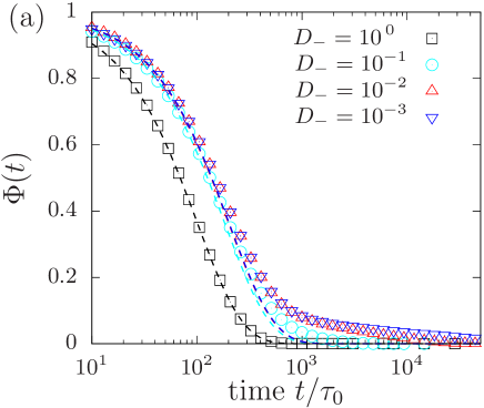
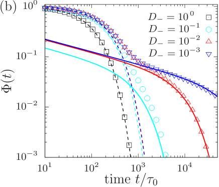
Figure 2: (Color online) Relaxation function $\Phi(t)$ as a function of time $t$ in (a) semi-log form and (b) log-log form. Time is measured in units of $\tau_{0}$, a cutoff time for short trap times (See Appendix B for details). The values of $\Phi(t)$ are obtained by numerical simulations of Eq. (1) with the spatial dimension $d=1$. The initial ensemble for $D(t)$ is assumed to be in equilibrium, and the initial distribution for $r(t)$ is given by the local equilibrium ensemble. Results for four different values of the slow diffusion coefficient $D_{-}$ are displayed: $D_{-}/D_{+}=10^{0}\,(\text{square}),10^{-1}\,(\text{circle}),10^{-2}\,(\text{triangle up}),$ and $10^{-3}\,(\text{triangle down})$. The damping coefficient $u$ is set as $u=0.01/D_{+}\tau_{0}$. The scaling exponents $\alpha_{-}$ of the power law distribution $\rho^{-}(\tau)$ is set as $\alpha_{-}=1.25$. In contrast, $\rho^{+}(\tau)$ is assumed to be the exponential distribution with $\mu_{+}=\mu_{-}$. The dashed and solid lines are the theoretical predictions for the short and long time regimes, respectively [Eq. (53) and Eq. (55)]. There are no fitting parameters.

IV.2.1 Equilibrium ensemble

If the sojourn-time distributions $\rho^{\pm}(\tau)$ follow the power-law distributions with finite means $\mu_{\pm}$, their Laplace transforms ($\tau\leftrightarrow\sigma$) can be expressed as

$$\hat{\rho}^{\pm}(\sigma)\underset{\sigma\to 0}{\simeq}1-\mu_{\pm}\sigma+a_{\pm}\sigma^{\alpha_{\pm}}+o(\sigma^{\alpha_{\pm}}),$$ (48)

where $1<\alpha_{-}<\alpha_{+}\leq 2$, and $o(\sigma^{\alpha_{\pm}})$ is Landau’s notation. When $\alpha_{+}=2$, $\rho^{+}(\tau)$ is the exponential distribution. Note also that the fast switching assumption between the two states, $z_{\pm}\ll k_{\pm}=1/\mu_{\pm}$, is necessary to use the expansion in Eq. (48) with $\sigma=z_{\pm}$. In addition to this condition, we assume that $\mu_{\pm}z_{\pm}\gg a_{\pm}z_{\pm}^{\alpha_{\pm}}$. The auxiliary function $\tilde{\rho}^{\pm}(\sigma)$ [Eq. (42)] is then given by

$$\tilde{\rho}^{\pm}(\sigma)\underset{\sigma\to 0}{\simeq}\mu_{\pm}\sigma-a_{\pm}\sigma^{\alpha_{\pm}}+o(\sigma^{\alpha_{\pm}}).$$ (49)

The function $\breve{f}^{D}(u;s|w^{\mathrm{eq}})$ can be given in a form similar to Eq. (III.3). In fact, $\breve{f}^{D}(u;s|w^{\mathrm{eq}})$ can be obtained just by replacing $\hat{\rho}^{\pm,0}$ and $p_{\pm}^{0}$ in Eq. (III.3) with $\hat{\rho}^{\pm,\mathrm{eq}}$ and $p_{\pm}^{\mathrm{eq}}$, respectively. Furthermore, by using $\hat{\rho}^{\pm,\mathrm{eq}}(z_{\pm})=\tilde{\rho}^{\pm}(z_{\pm})/(\mu_{\pm}z_{\pm})$ [see Eq. (76)] and Eq. (17), we rewrite Eq. (III.3) as

$$\!\!\!\!\!\breve{f}^{D}(u;s|w^{\mathrm{eq}})= \frac{\mu_{+}+\mu_{-}}{\mu_{+}z_{+}+\mu_{-}z_{-}}+\frac{\left(\frac{1}{z_{+}}-\frac{1}{z_{-}}\right)^{2}}{\mu_{+}+\mu_{-}}\left[\frac{\mu_{+}\mu_{-}z_{+}z_{-}}{\mu_{+}z_{+}+\mu_{-}z_{-}}-\frac{\tilde{\rho}^{+}(z_{+})\tilde{\rho}^{-}(z_{-})}{\tilde{\rho}^{+}(z_{+})+\tilde{\rho}^{-}(z_{-})-\tilde{\rho}^{+}(z_{+})\tilde{\rho}^{-}(z_{-})}\right].$$ (50)

This expression for the equilibrium ensemble is valid for any sojourn-time PDFs $\rho^{\pm}(\tau)$ with finite means $\mu_{\pm}$.

Now, substituting $\tilde{\rho}^{\pm}(z_{\pm})\simeq\mu_{\pm}z_{\pm}-a_{\pm}z_{\pm}^{\alpha_{\pm}}$ into Eq. (50), we have a formula for the power-law sojourn-time PDFs as

$$\breve{f}^{D} (u;s|w^{\mathrm{eq}})\simeq\frac{1}{s+\left\langle D\right\rangle_{\mathrm{eq}}u}$$

$$+\frac{(\Delta Du)^{2}\left(a_{-}\mu_{+}^{2}z_{-}^{\alpha_{-}-2}+a_{+}\mu_{-}^{2}z_{+}^{\alpha_{+}-2}\right)}{\mu^{3}(s+\left\langle D\right\rangle_{\mathrm{eq}}u)^{2}},$$ (51)

where $\mu$ and $\Delta D$ are defined by $\mu:=\mu_{+}+\mu_{-}$, and $\Delta D:=D_{+}-D_{-}$, respectively.

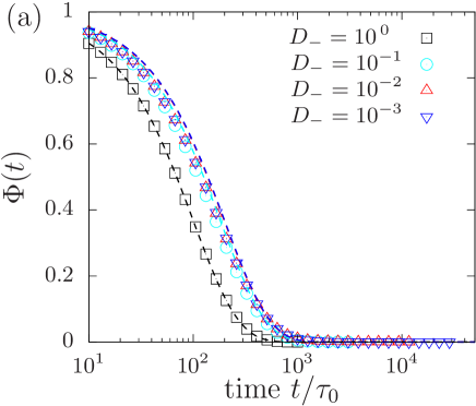
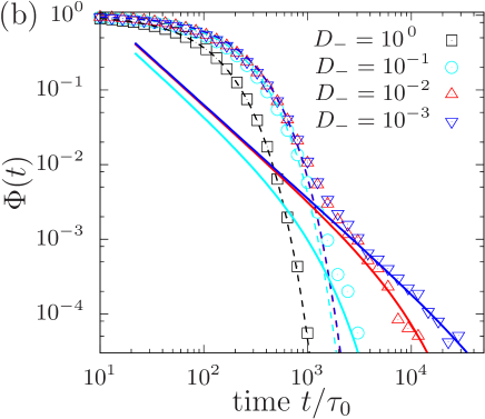
Figure 3: (Color online) Relaxation function $\Phi(t)$ as a function of time $t$ in (a) semi-log form and (b) log-log form. The initial ensemble for $D(t)$ is assumed to be the typical non-equilibrium ensemble $w^{\mathrm{neq}}$ with the initial fractions $p_{\pm}^{0}=p_{\pm}^{\mathrm{eq}}$. The other parameter values and the initial ensemble for $r(t)$ are exactly the same as those in Fig. 2. The dashed and solid lines are the theoretical predictions for the short and long time regimes, respectively [Eq. (59) and Eq. (61)]. There are no fitting parameters.

For $s\sim D_{+}u$, the first term in Eq. (IV.2.1) is dominant over the second, and thus the latter can be neglected. Therefore, we have

$$\breve{f}^{D}(u;s|w^{\mathrm{eq}})\simeq\frac{1}{s+\left\langle D\right\rangle_{\mathrm{eq}}u},$$ (52)

or, by the Laplace inversion, we obtain

$$\hat{f}^{D}(u;t|w^{\mathrm{eq}})\simeq e^{-\left\langle D\right\rangle_{\mathrm{eq}}ut}.$$ (53)

Thus, at the short time scale $t\sim 1/D_{+}u$, the exponential relaxation is observed.

However, for $s\ll D_{+}u$, we have $s+\left\langle D\right\rangle_{\mathrm{eq}}\sim\left\langle D\right\rangle_{\mathrm{eq}}$ and $z_{+}\sim D_{+}u$. The constant terms must be exponentially small after the Laplace inversion, and thus, we have from Eq. (IV.2.1)

$$\breve{f}^{D}(u;s|w^{\mathrm{eq}})\simeq\frac{a_{-}}{\mu}\left(\frac{\mu_{+}\Delta D}{\mu\left\langle D\right\rangle_{\mathrm{eq}}}\right)^{2}z_{-}^{\alpha_{-}-2}.$$ (54)

By the Laplace inversion, we have the following expression in the time domain $t\gg 1/D_{+}u$

$$\hat{f}^{D}(u;t|w^{\mathrm{eq}})\simeq\frac{a_{-}}{\mu}\left(\frac{\mu_{+}\Delta D}{\mu\left\langle D\right\rangle_{\mathrm{eq}}}\right)^{2}\frac{e^{-D_{-}ut}t^{1-\alpha_{-}}}{|\Gamma(2-\alpha_{-})|}.$$ (55)

Thus, in the case $1<\alpha_{-}<2$, the relaxation function exhibits the exponential decay at the short time scale [Eq. (53)], whereas it exhibits the power-law decay with an exponential cutoff at the long time scale [Eq. (55)]. As shown in Fig. 2, these theoretical results are consistent with numerical simulations. It is possible to show that Eqs. (52)– (55) are valid also for $\alpha_{\pm}>2$ (it should be assumed that $\alpha_{-}<\alpha_{+}$ and that $\alpha_{-}$ is not an integer). Thus, the power-law dacay $1/t^{1-\alpha_{-}}$ with any values of $\alpha_{-}>1$ is possible in principle. However, for $\alpha_{-}>2$, the decay is relatively fast, and therefore it might be difficult to observe the predicted power-law decay behavior even in numerical simulations.

IV.2.2 Non-equilibrium ensemble

The relaxation function for the typical non-equilibrium ensemble $w^{\mathrm{neq}}(\tau_{1})=p_{+}^{0}\rho^{+}(\tau_{1})+p_{-}^{0}\rho^{-}(\tau_{1})$ with $p_{+}^{0}+p_{-}^{0}=1$ can be derived in the same way as the case of the equilibrium ensemble. By replacing $\hat{\rho}^{\pm,0}(z_{\pm})$ in Eq. (III.3) with $\hat{\rho}^{\pm}(z_{\pm})$, and substituting Eqs. (48) and (49) into the resulting equation, we obtain

$$\breve{f}^{D} (u;s|w^{\mathrm{neq}})=\frac{\mu_{+}+\mu_{-}}{\mu_{+}z_{+}+\mu_{-}z_{-}}$$

$$+ \frac{z_{+}-z_{-}}{z_{+}z_{-}}\left[\frac{p_{-}^{0}\mu_{+}z_{+}-p_{+}^{0}\mu_{-}z_{-}}{\mu_{+}z_{+}+\mu_{-}z_{-}}+\frac{p_{+}^{0}\tilde{\rho}^{-}(z_{-})-p_{-}^{0}\tilde{\rho}^{+}(z_{+})+(p_{-}^{0}-p_{+}^{0})\tilde{\rho}^{+}(z_{+})\tilde{\rho}^{-}(z_{-})}{\tilde{\rho}^{+}(z_{+})+\tilde{\rho}^{-}(z_{-})-\tilde{\rho}^{+}(z_{+})\tilde{\rho}^{-}(z_{-})}\right].$$ (56)

Note that this expression for the typical non-equilibrium ensemble $w^{\mathrm{neq}}$ is valid for any sojourn-time PDF $\rho^{\pm}(\tau)$ with finite means $\mu_{\pm}$.

Now, substituting $\tilde{\rho}^{\pm}(z_{\pm})\simeq\mu_{\pm}z_{\pm}-a_{\pm}z_{\pm}^{\alpha_{\pm}}$, we have a formula for the power-law sojourn-time PDFs as

$$\breve{f}^{D}(u;s|w^{\mathrm{neq}}) \simeq\frac{1}{s+\left\langle D\right\rangle_{\mathrm{eq}}u}$$

$$+ \frac{\Delta Du\left(\mu_{-}a_{+}z_{+}^{\alpha_{+}-1}-\mu_{+}a_{-}z_{-}^{\alpha_{-}-1}\right)}{\mu^{2}\left(s+\left\langle D\right\rangle_{\mathrm{eq}}u\right)^{2}}.$$ (57)

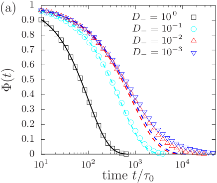
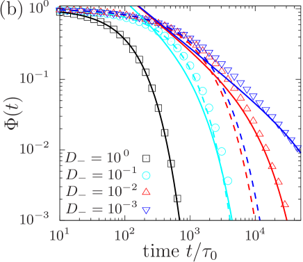
Figure 4: (Color online) Relaxation function $\Phi(t)$ as a function of time $t$ in (a) semi-log form and (b) log-log form. The initial ensemble for $D(t)$ is assumed to be the non-equilibrium ensemble $w^{\mathrm{neq}}$ with the initial fractions $p_{\pm}^{0}=0.5$. The scaling exponent $\alpha_{-}$ of the power law distribution $\rho^{-}(\tau)$ is set as $\alpha_{-}=0.75$. In contrast, $\rho^{+}(\tau)$ is assumed to be the exponential distribution with $\mu_{+}=2\tau_{0}$. The other parameter values and the initial ensemble for $r(t)$ are exactly the same as those in Fig. 2. The dashed and solid lines are the theoretical predictions for the short and long time regimes, respectively [Eqs. (63) and (65)]. There is no fitting parameters.

For $s\sim D_{+}u$, the first term in Eq. (57) is dominant over the second, and thus the latter can be neglected. Therefore, we have

$$\breve{f}^{D}(u;s|w^{\mathrm{neq}})\simeq\frac{1}{s+\left\langle D\right\rangle_{\mathrm{eq}}u}$$ (58)

or, by the Laplace inversion, we obtain

$$\hat{f}^{D}(u;t|w^{\mathrm{neq}})\simeq e^{-\left\langle D\right\rangle_{\mathrm{eq}}ut}.$$ (59)

Thus, at the short time scale $t\sim 1/D_{+}u$, the exponential relaxation, which is exactly the same as that in the equilibrium ensemble [Eq. (53)], is observed.

However, for $s\ll D_{+}u$, the constant terms can be neglected because they are exponentially small after the Laplace inversion, and thus we have

$$\breve{f}^{D}(u;s|w^{\mathrm{neq}})\simeq-\frac{a_{-}\mu_{+}\Delta D}{\mu^{2}\left\langle D\right\rangle_{\mathrm{eq}}^{2}u}z_{-}^{\alpha_{-}-1},$$ (60)

or by the Laplace inversion, we obtain a power-law decay again for the long time regime $t\gg 1/D_{+}u$ as

$$\hat{f}^{D}(u;t|w^{\mathrm{neq}})\simeq\frac{a_{-}\mu_{+}\Delta D}{\mu^{2}\left\langle D\right\rangle^{2}_{\mathrm{eq}}u}\frac{e^{-D_{-}ut}t^{-\alpha_{-}}}{|\Gamma(1-\alpha_{-})|}.$$ (61)

As shown in Fig. 3, these theoretical results are consistent with numerical simulation. These results [Eqs. (58)– (61)] are valid also for $\alpha_{\pm}>2$ (it should be assumed that $\alpha_{-}<\alpha_{+}$ and that $\alpha_{-}$ is not an integer).

As in the case of the equilibrium ensemble, the relaxation for the non-equilibrium ensemble is given by the exponential decay at the short time scale [Eq. (59)], whereas power-law decay with an exponential cutoff at the long time scale [Eq. (61)]. Thus, the behavior of both ensembles are qualitatively similar except that the power-law decay is slower for the equilibrium ensemble than for the non-equilibrium ensemble. In fact, the power-law index for equilibrium ensemble is greater by one than that for the non-equilibrium ensemble [See Eqs. (55) and (61)]. This difference is due to the fact that the power-law index of the initial sojourn-time PDF for the equilibrium ensemble is smaller by one than that for the non-equilibrium ensemble [See Eq. (87)]. This difference of power-law exponents in the initial sojourn-time PDFs often provides a remarkable initial-ensemble dependence of physical observables such as the correlation function and the diffusion coefficient Akimoto and Aizawa (2007); Akimoto et al. (2018).

IV.3 Power-law distribution: $0<\alpha_{-}<1$

Finally, let us study the case in which $0<\alpha_{-}<1$. In this case, the equilibrium distribution $\rho^{-,\mathrm{eq}}(\tau)$ no longer exists, because the mean value of $\rho^{-}(\tau)$ diverges. Hence, we consider only the non-equilibrium ensemble $w^{\mathrm{neq}}$. On the other hand, $\alpha_{+}$ is assumed to be $1<\alpha_{+}\leq 2$ (For $0<\alpha_{+}<1$, we can have similar results with different scaling exponents. But the behavior for these two cases are qualitatively the same, and thus here we focus only on the case $1<\alpha_{+}\leq 2$). In addition to the assumptions for $\hat{\rho}^{+}(z_{+})$ used in the previous subsection, we further assume that $a_{-}z_{-}^{\alpha_{-}}\ll 1$; this condition is necessary for the expansion given in Eq. (85).

The double Laplace transform $\breve{f}^{D}(u;s|w^{\mathrm{neq}})$ is obtained by replacing $\hat{\rho}^{\pm,0}(z_{\pm})$ in Eq. (III.3) with $\hat{\rho}^{\pm}(z_{\pm})$. Substituting $\hat{\rho}^{\pm}(z_{\pm})\simeq 1$, $\tilde{\rho}^{+}(z_{+})\simeq\mu_{+}z_{+}$ and $\tilde{\rho}^{-}(z_{-})\simeq a_{-}z_{-}^{\alpha_{-}}$ into this equation, we have for $s\sim D_{+}u$

$$\breve{f}^{D}(u;s|w^{\mathrm{neq}})\simeq\frac{1}{z_{-}}-\frac{\mu_{+}}{a_{-}}\frac{\Delta Du}{z_{-}^{1+\alpha_{-}}}.$$ (62)

Strictly speaking, higher order terms should have been taken into account in this calculation, but the final result is unchanged because the higher order terms are canceled out. The Laplace inversion of Eq. (62) gives

$$\hat{f}^{D}(u;t|w^{\mathrm{neq}}) \simeq e^{-D_{-}ut}\left[1-\frac{\mu_{+}}{a_{-}}\frac{\Delta Du}{\Gamma(1+\alpha_{-})}t^{\alpha_{-}}\right]$$

$$\simeq e^{-D_{-}ut-\frac{\mu_{+}}{a_{-}}\frac{\Delta Du}{\Gamma(1+\alpha_{-})}t^{\alpha_{-}}}.$$ (63)

Thus, the relaxation function is given in a stretched-exponential form.

However, for $s\ll D_{+}u$, we have the following formula from the equation obtained by replacing $\hat{\rho}^{\pm,0}(z_{\pm})$ in Eq. (III.3) with $\hat{\rho}^{\pm}(z_{\pm})$

$$\breve{f}^{D}(u;s|w^{\mathrm{neq}})\simeq\frac{\Delta D}{D_{+}}\frac{a_{-}}{\mu_{+}}\frac{z_{-}^{\alpha_{-}-1}}{D_{+}u},$$ (64)

where we also assumed that $z_{-}^{\alpha_{-}}\ll D_{+}u$ (if this condition is not satisfied, the power-law regime vanishes). The Laplace inversion gives

$$\hat{f}^{D}(u;t|w^{\mathrm{neq}})\simeq\frac{\Delta D}{D_{+}^{2}u}\frac{a_{-}}{\mu_{+}}\frac{e^{-D_{-}ut}}{\Gamma(1-\alpha_{-})t^{\alpha_{-}}}.$$ (65)

Thus, in the case $0<\alpha_{-}<1$, the relaxation function exhibits the stretched-exponential decay at the short time scale, whereas the power-law decay with an exponential cutoff at the long time scale. As shown in Fig. 4, these theoretical results are consistent with numerical simulation.

V Discussion

Recently, Brownian motion with fluctuating diffusivity has been investigated intensively. To characterize such processes, various kinds of correlation functions are used. One of the most frequently used functions might be an ergodicity breaking parameter, which is a fourth order correlation function in terms of the position vector Uneyama et al. (2012, 2015, 2019); Miyaguchi et al. (2016); Miyaguchi (2017); Cherstvy et al. (2013); Cherstvy and Metzler (2016); Metzler et al. (2014). For the case of the LEFD, it is shown that the fluctuating diffusivity cannot be detected with the second order correlation including the MSD Miyaguchi (2017).

In this work, we have studied the relaxation function $\hat{f}^{R}(u;t|w^{0})$. This quantity can be interpreted as a second order position correlation function [Eq. (5)] for the OUFD, and as the self-intermediate scattering function [Eq. (15)] for the LEFD. This correlation function characterizes the fluctuating diffusivity in the sense that it is a Laplace transformation of the integral diffusivity $\int_{0}^{t}dt^{\prime}D(t^{\prime})$.

Under the assumption that the system has two diffusive states, we have derived a general formula [Eq. (III.3)] for the relaxation function $\hat{f}^{R}(u;t|w^{0})$ in terms of the sojourn-time PDFs $\rho^{\pm}(\tau)$. In particular, if the sojourn-time PDF of the slow state is given by a power-law distribution with the index $\alpha_{-}$, the relaxation function at the short time scales shows the exponential relaxation for $1<\alpha_{-}<2$, or the stretched-exponential relaxation for $0<\alpha_{-}<1$. In contrast, at the long time scales, the relaxation function shows a power law decay with an exponential cutoff.

The fact that our model can reproduce the stretched-exponential relaxation function is quite interesting. The stretched-exponential type relaxation behavior has been widely observed in various systems, and generally interpreted as the signature of a heterogeneity. Various models have been proposed to interpret the microscopic origin of the stretched-exponential relaxation Palmer et al. (1984); Odagaki and Hiwatari (1990); Ngai and Rendell (1993); Phillips (1996); Metzler and Klafter (2000). In most of such models, power-law type distributions for some physical quantities such as the waiting time are assumed.

Our model also assumes the power-law distribution for the sojourn time, and thus, in this aspect, it is similar to the conventional models. In particular, it would be worth mentioning a relation of the present model with the quenched-trap model studied in Ref. Odagaki and Hiwatari (1990). Statistical properties of the quenched-trap model with the spatial dimension $d>2$ is asymptotically the same as those of the continuous-time random walks Machta (1985). On the other hand, the LEFD also reduces to the continuous-time random walk in the limit $\mu_{+}\to 0$ with $D_{+}\mu_{+}=\mathrm{const}$ and $D_{-}=0$ Uneyama et al. (2015). Thus, the generation mechanism of the stretched-exponential relaxation (as well as the anomalous diffusion Miyaguchi et al. (2016)) in the present model may be similar to that in the quenched-trap model Odagaki and Hiwatari (1990).

In spite of these similarities between our model and previously studied systems, however, our model might have some advantages in that its dynamics is described by simple equations [Eqs. (1) and (7)]. This is in contrast to some conventional models, where the dynamic equation and the time evolution rule are not expressed in clear and simple equations. We expect that the combination of our model and experimental relaxation data can be employed to interpret molecular-level dynamics of heterogeneous systems. In fact, a model similar to ours was utilized to reproduce results of numerical simulations for glassy systems and supercooled liquids Chaudhuri et al. (2007); Helfferich et al. (2018).

Moreover, the stretched-exponential relaxation is obtained in our model when the equilibrium distribution $\rho^{-,\mathrm{eq}}(\tau)$ does not exist. This means that, the system is not in equilibrium, if it shows the stretched exponential type relaxation. This seems to be consistent with a naive expectation that the dynamic heterogeneity is a precursor of a glass transition which is clearly in non-equilibrium.

As we mentioned, the stretched-exponential relaxation is observed ubiquitously in complex and highly concentrated systems , but its origin is still unclear Phillips (1996). The stretched-exponential relaxation is often expressed as $e^{-(t/\bar{\tau})^{\beta}}$ where $\bar{\tau}$ and $\beta$ are constants; $\beta$ is typically around $0.5$ (experimental values are about $0.4\lesssim\beta\lesssim 0.6$). In our model, this exponent is simply given as $\beta=\alpha_{-}$, and therefore it reflects the tail of the sojourn-time PDF of the slow state at the long time region. This result implies that the power-law sojourn-time PDF for the slow state plays a fundamental role in emergence of the stretched-exponential relaxation. The power-law sojourn-time PDF, which is assumed in our model, is also generally observed in crowded systems Doliwa and Heuer (2003); Helfferich et al. (2014). Thus, our model might bridge a gap between these commonly observed phenomena: the power-law sojourn times and stretched-exponential relaxation.

Although it seems that the fast state plays a minor role, its property affects the characteristic relaxation time; in our model, the characteristic relaxation time $\bar{\tau}$ is given as $\bar{\tau}=[\mu_{+}\Delta Du/a_{-}\Gamma(1+\alpha_{+})]^{1/\alpha_{-}}$. Thus, the characteristic time scale depends on various parameters such as the sojourn-time PDF of the fast state and the two diffusion coefficients.

Appendix A Equilibrium ensemble

As explained in Sec. II, the initial ensemble is fully specified by the PDF of the first sojourn time $\tau_{1}$ [Recall that the initial distribution of the position $\bm{r}(0)$ is unimportant in investigating the relaxation function $\Phi(t)$]. We derive an explicit expression for the Laplace transform of the equilibrium ensemble $\hat{\rho}^{\pm,\mathrm{eq}}(\sigma):=\int_{0}^{\infty}d\tau e^{-\tau\sigma}\rho^{\pm,\mathrm{eq}}(\tau)$.

The equilibrium ensemble can be derived from a forward-recurrence-time PDF. A forward-recurrence time is a sojourn time until the next transition from some elapsed time $t^{\prime}>0$ Godrèche and Luck (2001). Here, we study the forward-recurrence-time PDF $w_{\pm}(\tau;t^{\prime}|w^{0})$, from which we obtain the equilibrium ensemble by taking a limit $t^{\prime}\to\infty$.

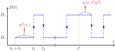
Figure 5: (Color online)Schematic illustration of the forward-recurrence time $\tau$. A realization started from the initial ensemble $w^{0}(\tau_{1})$ is displayed as an example. The first sojourn time $\tau_{1}$ follows $w^{0}(\tau_{1})=w_{+}^{0}(\tau_{1})+w_{-}^{0}(\tau_{1})$ [See Eq. (20)]. Then, the sojourn time $\tau$ at time $t^{\prime}$ until the next transition follows $w(\tau;t^{\prime}|w^{0}):=w_{+}(\tau;t^{\prime}|w^{0})+w_{-}(\tau;t^{\prime}|w^{0})$.

A.1 PDF for forward-recurrence time

The forward-recurrence-time PDF $w_{\pm}(\tau;t^{\prime}|w^{0})d\tau$ is a joint probability that (i) the state is $\pm$ at time $t^{\prime}$, and (ii) the sojourn time from $t^{\prime}$ until the next transition is in an interval $[\tau,\tau+d\tau]$, given that the process starts with $w^{0}(\tau_{1})$ at $t=0$. Here, $\tau$ is called the forward-recurrence time, and it is illustrated in Fig. 5.

To obtain the forward-recurrence-time PDF, we further define the following PDFs for $n=0,1,\dots$:

$$w_{\pm,n}(\tau;t^{\prime}|w^{0}):=\left\langle\delta\left(\tau-(t_{n+1}-t^{\prime})\right)I\left(t_{n}<t^{\prime}<t_{n+1}\right)\delta_{\pm}\right\rangle,$$ (66)

where $w_{\pm,n}(\tau;t^{\prime}|w^{0})d\tau$ is a joint probability that (i) the state is $\pm$ at $t=0$, (ii) there are $n$ transitions until time $t^{\prime}$, and (iii) the sojourn time at time $t^{\prime}$ is in an interval $[\tau,\tau+d\tau]$, given that the process starts with $w^{0}(\tau_{1})$ at $t=0$.

The double Laplace transforms $\breve{w}_{\pm,n}(\sigma;s|w^{0}):=\int_{0}^{\infty}dt^{\prime}e^{-t^{\prime}s}\int_{0}^{\infty}d\tau e^{-\tau\sigma}w_{\pm,n}(\tau;t^{\prime}|w^{0})$ with respect to $\tau$ and then $t^{\prime}$ result in ($\tau\leftrightarrow\sigma$ and $t^{\prime}\leftrightarrow s$)

$$\breve{w}_{\pm,n}(\sigma;s|w^{0}) =\left\langle\frac{\delta_{\pm}e^{-t_{n}s}}{s-\sigma}\left(e^{-\sigma\tau_{n+1}}-e^{-s\tau_{n+1}}\right)\right\rangle$$

$$=\begin{cases}\displaystyle\frac{\left\langle\delta_{\pm}e^{-\sigma\tau_{1}}\right\rangle-\left\langle\delta_{\pm}e^{-s\tau_{1}}\right\rangle}{s-\sigma}&(n=0),\\[5.69046pt] \displaystyle\left\langle\delta_{\pm}e^{-st_{n}}\right\rangle\frac{\left\langle e^{-\sigma\tau_{n+1}}\right\rangle_{\pm}-\left\langle e^{-s\tau_{n+1}}\right\rangle_{\pm}}{s-\sigma}&(n=1,2,\dots),\end{cases}$$ (67)

where $\left\langle\dots\right\rangle_{\pm}$ is a conditional average for a given initial state $\pm$. The ensemble averages in the above equation can be expressed with the Laplace transforms of the initial ensemble $\hat{w}_{\pm}^{0}(s)$ and the sojourn-time PDFs $\hat{\rho}^{\pm}(s)$. In fact, we have

$$\left\langle\delta_{\pm}e^{-st_{2n}}\right\rangle =\left\langle\delta_{\pm}\right\rangle\left\langle e^{-s\tau_{1}}\right\rangle_{\pm}\left\langle e^{-s\tau_{2}}\right\rangle_{\pm}\times\dots\times\left\langle e^{-s\tau_{2n}}\right\rangle_{\pm}$$

$$=\hat{w}_{\pm}^{0}(s)\hat{\rho}^{n-1}(s)\hat{\rho}^{\mp}(s),$$ (68)

$$\left\langle\delta_{\pm}e^{-s\tau_{2n-1}}\right\rangle =\left\langle\delta_{\pm}\right\rangle\left\langle e^{-s\tau_{1}}\right\rangle_{\pm}\left\langle e^{-s\tau_{2}}\right\rangle_{\pm}\times\dots\times\left\langle e^{-s\tau_{2n-1}}\right\rangle_{\pm}$$

$$=\hat{w}_{\pm}^{0}(s)\hat{\rho}^{n-1}(s),$$ (69)

for $n=1,2,\cdots$, where $\hat{\rho}(s):=\hat{\rho}^{+}(s)\hat{\rho}^{-}(s)$ and $\left\langle\dots\right\rangle_{\pm}$ is a conditional average under the condition that the initial state is $\pm$. Then, using Eqs. (68) and (69) in Eq. (67), we have

$$\breve{w}_{\pm,0}(\sigma;s|w^{0}) =\dfrac{\hat{w}_{\pm}^{0}(\sigma)-\hat{w}_{\pm}^{0}(s)}{s-\sigma},$$ (70)

$$\breve{w}_{\pm,2n}(\sigma;s|w^{0}) =\hat{w}^{0}_{\pm}(s)\hat{\rho}^{n-1}(s)\hat{\rho}^{\mp}(s)\dfrac{\hat{\rho}^{\pm}(\sigma)-\hat{\rho}^{\pm}(s)}{s-\sigma},$$ (71)

$$\breve{w}_{\pm,2n-1}(\sigma;s|w^{0}) =\hat{w}^{0}_{\pm}(s)\hat{\rho}^{n-1}(s)\dfrac{\hat{\rho}^{\mp}(\sigma)-\hat{\rho}^{\mp}(s)}{s-\sigma},$$ (72)

for $n=1,2,\dots$.

Because the Laplace transform of the forward-recurrence-time PDF, $w_{\pm}(\tau;t^{\prime}|w^{0})$, is given by $\breve{w}_{\pm}(\sigma;s|w^{0})=\sum_{n=0}^{\infty}[\breve{w}_{\pm,2n}(\sigma;s|w^{0})+\breve{w}_{\mp,2n+1}(\sigma;s|w^{0})]$, we have

$$\breve{w}_{\pm}(\sigma;s|w^{0}) =\frac{\hat{w}^{0}_{\pm}(\sigma)-\hat{w}^{0}_{\pm}(s)}{s-\sigma}$$

$$+ \frac{\hat{w}^{0}_{\pm}(s)\hat{\rho}^{\mp}(s)+\hat{w}^{0}_{\mp}(s)}{1-\hat{\rho}(s)}\frac{\hat{\rho}^{\pm}(\sigma)-\hat{\rho}^{\pm}(s)}{s-\sigma}.$$ (73)

Equation (A.1) is a general expression of the forward-recurrence-time PDF for the alternating renewal processes.

A.2 Equilibrium ensemble

If both $\mu_{+}$ and $\mu_{-}$ exist, it follows from Eq. (A.1) that

$$\lim_{t^{\prime}\to\infty}\hat{w}_{\pm}(\sigma;t^{\prime}|w^{0})=\lim_{s\to 0}s\breve{w}_{\pm}(\sigma;s|w^{0})=p_{\pm}^{\mathrm{eq}}\frac{1-\hat{\rho}^{\pm}(\sigma)}{\mu_{\pm}\sigma}.$$ (74)

Since the above limit $t^{\prime}\to\infty$ is equivalent to putting the start time of the process to $-\infty$, the limitting function should be equivalent to the equilibrium ensemble $\hat{w}^{\mathrm{eq}}_{\pm}(\sigma)$:

$$\hat{w}_{\pm}^{\mathrm{eq}}(\sigma):=p_{\pm}^{\mathrm{eq}}\hat{\rho}^{\pm,\mathrm{eq}}(\sigma)$$ (75)

where $\hat{\rho}^{\pm,\mathrm{eq}}(\sigma)$ is defined as

$$\hat{\rho}^{\pm,\mathrm{eq}}(\sigma)=\frac{1-\hat{\rho}^{\pm}(\sigma)}{\mu_{\pm}\sigma},$$ (76)

Hence, the equilibrium PDF exists only if $\mu_{\pm}$ is finite as explained in the main text. Note also that the equilibrium ensemble [Eq. (74)] does not depend on the initial ensemble $w^{0}$, as expected.

A.2.1 Exponential distribution

If the sojourn-time PDFs are given by the exponential distributions

$$\rho^{\pm}(\tau)=\frac{1}{\mu_{\pm}}\exp\left(-\frac{\tau}{\mu_{\pm}}\right)=k_{\pm}\exp\left(-k_{\pm}{\tau}\right),$$ (77)

we have its Laplace transforms ($\tau\leftrightarrow\sigma$) as

$$\hat{\rho}^{\pm}(\sigma)=\frac{1}{1+\mu_{\pm}\sigma}=\frac{k_{\pm}}{k_{\pm}+\sigma}.$$ (78)

In this case, the equilibrium PDF [Eq. (76)] is equivalent to $\rho^{\pm}(\tau)$, i.e., it is easy to check

$$\hat{\rho}^{\pm,\mathrm{eq}}(\sigma)=\frac{1-\hat{\rho}^{\pm}(\sigma)}{\mu_{\pm}\sigma}=\hat{\rho}^{\pm}(\sigma).$$ (79)

Thus, the equilibrium ensemble is given by $p_{+}^{\mathrm{eq}}\rho_{+}(\tau_{1})+p_{-}^{\mathrm{eq}}\rho_{-}(\tau_{1})$.

More generally, the forward-recurrence-time PDF for the exponential sojourn times is calculated as follows. Here, let us assume that the initial ensemble is the typical non-equilibrium ensemble, i.e., $w_{\pm}^{\mathrm{neq}}(\tau_{1})=p_{+}^{0}\rho_{+}(\tau_{1})+p_{-}^{0}\rho_{-}(\tau_{1})$, where $p_{\pm}^{0}$ are the initial fractions with the constraint $p_{+}^{0}+p_{-}^{0}=1$. Then, after some straightforward calculations, the forward-recurrence-time PDF [Eq. (A.1)] is given as

$$\breve{w}_{\pm}(\sigma;s|w^{\mathrm{neq}})=\frac{1}{1+\mu_{\pm}\sigma}\left[\frac{p_{\pm}^{\mathrm{eq}}}{s}+\frac{p_{\pm}^{0}-p_{\pm}^{\mathrm{eq}}}{s+\frac{\mu_{+}+\mu_{-}}{\mu_{+}\mu_{-}}}\right].$$ (80)

The double Laplace inversions give

$$w_{\pm}(\tau;t^{\prime}|w^{\mathrm{neq}})=p_{\pm}(t^{\prime})\frac{e^{-\tau/\mu_{\pm}}}{\mu_{\pm}},$$ (81)

where $p_{\pm}(t^{\prime})$ are the fractions at time $t^{\prime}$, and are given as

$$p_{\pm}(t^{\prime}):=p_{\pm}^{\mathrm{eq}}+\left(p_{\pm}^{0}-p_{\pm}^{\mathrm{eq}}\right)e^{-\frac{\mu_{+}+\mu_{-}}{\mu_{+}\mu_{-}}t}.$$ (82)

From Eqs. (81) and (82), the forward-recurrence-time PDF at $t^{\prime}$ is also represented as

$$p_{+}(t^{\prime})\rho^{+}(\tau)+p_{-}(t^{\prime})\rho^{-}(\tau),$$ (83)

Thus, the forward-recurrence-time PDF with respect to the exponential distributions are also given by the exponential distributions, and only the fractions change with time. This is an outcome of the fact that the exponential distribution is Markovian. In addition, the fractions converge to the equilibrium fractions $p_{\pm}^{\mathrm{eq}}$ exponentially.

A.2.2 Power law distribution

The power law distribution is given by

$$\rho^{\pm}(\tau)\underset{\tau\to\infty}{\simeq}\frac{a_{\pm}}{|\Gamma(-\alpha_{\pm})|\tau^{1+\alpha_{\pm}}},$$ (84)

where $a_{\pm}$ is a scale factor and $\Gamma(-\alpha_{\pm})$ is the gamma function. Asymptotic forms of the Laplace transforms $\hat{\rho}_{\pm}(\sigma):=\int_{0}^{\infty}d\tau\,e^{-\tau\sigma}\rho_{\pm}(\tau)$ at small $\sigma$ are given by

$$\hat{\rho}_{\pm}(\sigma) \underset{\sigma\to 0}{\simeq}1-a_{\pm}\sigma^{\alpha_{\pm}}+o(\sigma^{\alpha_{\pm}}),\quad (0<\alpha_{\pm}<1)$$ (85)

$$\hat{\rho}_{\pm}(\sigma) \underset{\sigma\to 0}{\simeq}1-\mu_{\pm}\sigma+a_{\pm}\sigma^{\alpha_{\pm}}+o(\sigma^{\alpha_{\pm}}),\quad (1<\alpha_{\pm}<2)$$ (86)

where $\mu_{\pm}$ is the mean sojourn time of the state $\pm$.

Now, let us assume that the sojourn-time PDF is given by a power law distribution. For $0<\alpha_{\pm}<1$, the mean sojourn time $\mu_{\pm}$ diverges, and therefore the equilibrium ensemble [Eq. (75)] does not exist. In contrast, for $1<\alpha_{\pm}\leq 2$, the equilibrium ensemble exists and is given by

$$\hat{\rho}^{\pm,\mathrm{eq}}(\sigma)=\frac{1-\hat{\rho}^{\pm}(\sigma)}{\mu_{\pm}\sigma}\underset{\sigma\to 0}{\simeq}1-\frac{a_{\pm}}{\mu_{\pm}}\sigma^{\alpha_{\pm}-1},$$ (87)

where we used Eq. (86). The important point is that the power exponent of $\sigma$ in Eq. (87) is smaller by one than that in the sojourn-time PDF [Eq. (86)]. This means that the mean initial sojourn time of the equilibrium ensemble with $1<\alpha_{\pm}<2$ diverges.

Appendix B Simulation setup

In numerical simulations, we used a simple sojourn-time PDF defined as

$$\rho_{\pm}(\tau)=\frac{\alpha_{\pm}\tau_{0}^{\alpha_{\pm}}}{\tau^{1+\alpha_{\pm}}},\qquad(\tau_{0}\leq\tau<\infty)$$ (88)

where $\tau_{0}$ is a cutoff time for short trap times; we assume the same cutoff time for both $\rho_{+}(\tau)$ and $\rho_{-}(\tau)$. Then, by comparing Eq. (88) with Eq. (84), it is found that $a_{\pm}$ in Eq. (48) is given by $a_{\pm}=\tau_{0}^{\alpha_{\pm}}|\Gamma(1-\alpha_{\pm})|$. For $\alpha_{\pm}>1$, the mean sojourn times $\mu_{\pm}$ are given as

$$\mu_{\pm}=\frac{\alpha_{\pm}\tau_{0}}{\alpha_{\pm}-1}.$$ (89)

To simulate equilibrium processes, we have to generate initial ensembles which follow the first sojourn-time PDFs $\rho_{\pm}^{\mathrm{eq}}(t)$ [Eq. (76)]. This can be achieved with a method presented in Ref. Miyaguchi and Akimoto (2013). First, let $\Theta$ be a random variable following a PDF

$$\rho_{\pm}^{\prime}(\tau)=\frac{\tau}{\mu_{\pm}}\rho_{\pm}(\tau)=\frac{(\alpha_{\pm}-1)\tau_{0}^{\alpha_{\pm}-1}}{\tau^{\alpha_{\pm}}},\quad(\tau_{0}\leq\tau<\infty)$$ (90)

where Eq. (89) is used. Moreover, let $X$ be a random variable, which follows the uniform PDF on the interval $(0,1)$. Then, a random variable $X\Theta$ follows the PDF $\rho^{\pm,\mathrm{eq}}(\tau)$ (See Ref. Miyaguchi and Akimoto (2013) for a derivation).

The Langevin equation in Eq. (1), or its discretized form,

$$d\bm{r}(t)=-uD(t)\bm{r}(t)dt+\sqrt{2D(t)dt}\,\bm{\xi}(t),$$ (91)

can be transformed into a dimensionless form with

$$\tilde{\bm{r}}(t)=\frac{\bm{r}(t)}{\sqrt{D_{+}\tau_{0}}},\qquad\tilde{t}=\frac{t}{\tau_{0}},\qquad\tilde{u}=uD_{+}\tau_{0}$$ (92)

The remaining system parameters are $\alpha_{\pm}$, $\tilde{u}$ and the ratio $D_{-}/D_{+}$. In simulations, we set $D_{+}=1.0$ and $\tau_{0}=1$. For the numerical integration of the Langevin equation, the Euler method is employed Kloeden and Platen (2011).

References

- Dhont (1996) J. K. G. Dhont, An Introduction to Dynamics of Colloids (Elsevier, Amsterdam, 1996).
- Doi and Edwards (1986) M. Doi and S. F. Edwards, The Theory of Polymer Dynamics (Oxford University Press, Oxford, 1986).
- Bressloff and Newby (2013) P. C. Bressloff and J. M. Newby, Rev. Mod. Phys. 85, 135 (2013).
- Landau and Lifshitz (1987) L. D. Landau and E. Lifshitz, Fluid Mechanics, 2nd ed. (Elsevier, Oxford, 1987).
- Kim and Karrila (2013) S. Kim and S. J. Karrila, Microhydrodynamics: principles and selected applications (Dover, New York, 2013).
- Yamamoto and Onuki (1998a) R. Yamamoto and A. Onuki, Phys. Rev. Lett. 81, 4915 (1998a).
- Yamamoto and Onuki (1998b) R. Yamamoto and A. Onuki, Phys. Rev. E 58, 3515 (1998b).
- Parry et al. (2014) B. R. Parry, I. V. Surovtsev, M. T. Cabeen, C. S. O’Hern, E. R. Dufresne, and C. Jacobs-Wagner, Cell 156, 183 (2014).
- Uneyama et al. (2012) T. Uneyama, T. Akimoto, and T. Miyaguchi, J. Chem. Phys. 137, 114903 (2012).
- Uneyama et al. (2015) T. Uneyama, T. Miyaguchi, and T. Akimoto, Phys. Rev. E 92, 032140 (2015).
- Miyaguchi (2017) T. Miyaguchi, Phys. Rev. E 96, 042501 (2017).
- Chubynsky and Slater (2014) M. V. Chubynsky and G. W. Slater, Phys. Rev. Lett. 113, 098302 (2014).
- Manzo et al. (2015) C. Manzo, J. A. Torreno-Pina, P. Massignan, G. J. Lapeyre, M. Lewenstein, and M. F. Garcia Parajo, Phys. Rev. X 5, 011021 (2015).
- Chechkin et al. (2017) A. V. Chechkin, F. Seno, R. Metzler, and I. M. Sokolov, Phys. Rev. X 7, 021002 (2017).
- Jain and Sebastian (2017) R. Jain and K. L. Sebastian, J. Chem. Sci. 129, 929 (2017).
- Golding and Cox (2006) I. Golding and E. C. Cox, Phys. Rev. Lett. 96, 098102 (2006).
- Milo and Phillips (2015) R. Milo and R. Phillips, Cell biology by the numbers (Garland Science, New York, 2015).
- Uneyama et al. (2019) T. Uneyama, T. Miyaguchi, and T. Akimoto, Phys. Rev. E 99, 032127 (2019).
- Weber et al. (2010) S. C. Weber, A. J. Spakowitz, and J. A. Theriot, Phys. Rev. Lett. 104, 238102 (2010).
- Weigel et al. (2011) A. V. Weigel, B. Simon, M. M. Tamkun, and D. Krapf, Proc. Natl. Acad. Sci. U.S.A 108, 6438 (2011).
- Jeon et al. (2011) J.-H. Jeon, V. Tejedor, S. Burov, E. Barkai, C. Selhuber-Unkel, K. Berg-Sørensen, L. Oddershede, and R. Metzler, Phys. Rev. Lett. 106, 048103 (2011).
- Burov et al. (2011) S. Burov, J. Jeon, R. Metzler, and E. Barkai, Phys. Chem. Chem. Phys. 13, 1800 (2011).
- Tabei et al. (2013) S. M. A. Tabei, S. Burov, H. Y. Kim, A. Kuznetsov, T. Huynh, J. Jureller, L. H. Philipson, A. R. Dinner, and N. F. Scherer, Proc. Natl. Acad. Sci. U.S.A 110, 4911 (2013).
- Yamamoto et al. (2014) E. Yamamoto, T. Akimoto, M. Yasui, and K. Yasuoka, Sci. Rep. 4, 4720 (2014).
- He et al. (2008) Y. He, S. Burov, R. Metzler, and E. Barkai, Phys. Rev. Lett. 101, 058101 (2008).
- Meroz et al. (2010) Y. Meroz, I. M. Sokolov, and J. Klafter, Phys. Rev. E 81, 010101(R) (2010).
- Miyaguchi and Akimoto (2011) T. Miyaguchi and T. Akimoto, Phys. Rev. E 83, 031926 (2011).
- Leith et al. (2012) J. S. Leith, A. Tafvizi, F. Huang, W. E. Uspal, P. S. Doyle, A. R. Fersht, L. A. Mirny, and A. M. van Oijen, Proc. Natl. Acad. Sci. U.S.A 109, 16552 (2012).
- Detcheverry (2017) F. Detcheverry, Phys. Rev. E 96, 012415 (2017).
- Cox (1962) D. R. Cox, Renewal Theory (Methuen, London, 1962).
- Goychuk and Hänggi (2003) I. Goychuk and P. Hänggi, Phys. Rev. Lett. 91, 070601 (2003).
- Akimoto and Seki (2015) T. Akimoto and K. Seki, Phys. Rev. E 92, 022114 (2015).
- Miyaguchi et al. (2016) T. Miyaguchi, T. Akimoto, and E. Yamamoto, Phys. Rev. E 94, 012109 (2016).
- Odagaki and Hiwatari (1990) T. Odagaki and Y. Hiwatari, Phys. Rev. A 41, 929 (1990).
- Doliwa and Heuer (2003) B. Doliwa and A. Heuer, Phys. Rev. E 67, 030501(R) (2003).
- Helfferich et al. (2014) J. Helfferich, F. Ziebert, S. Frey, H. Meyer, J. Farago, A. Blumen, and J. Baschnagel, Phys. Rev. E 89, 042603 (2014).
- Sekimoto (2010) K. Sekimoto, Stochastic Energetics (Springer, Berlin, 2010).
- Hansen and McDonald (1990) J.-P. Hansen and I. R. McDonald, Theory of Simple Liquids (Elsevier, New York, 1990).
- Kob and Andersen (1995) W. Kob and H. C. Andersen, Phys. Rev. E 51, 4626 (1995).
- Berne and Pecora (2000) B. J. Berne and R. Pecora, Dynamic Light Scattering (Dover, New York, 2000).
- Godrèche and Luck (2001) C. Godrèche and J. M. Luck, J. Stat. Phys. 104, 489 (2001).
- Miyaguchi and Akimoto (2013) T. Miyaguchi and T. Akimoto, Phys. Rev. E 87, 032130 (2013).
- Akimoto and Aizawa (2007) T. Akimoto and Y. Aizawa, J Korean Phys. Soc. 50, 254 (2007).
- Akimoto et al. (2018) T. Akimoto, A. G. Cherstvy, and R. Metzler, Phys. Rev. E 98, 022105 (2018).
- Cherstvy et al. (2013) A. G. Cherstvy, A. V. Chechkin, and R. Metzler, New J. Phys. 15, 083039 (2013).
- Cherstvy and Metzler (2016) A. G. Cherstvy and R. Metzler, Phys. Chem. Chem. Phys. 18, 23840 (2016).
- Metzler et al. (2014) R. Metzler, J.-H. Jeon, A. G. Cherstvy, and E. Barkai, Phys. Chem. Chem. Phys. 16, 24128 (2014).
- Palmer et al. (1984) R. G. Palmer, D. L. Stein, E. Abrahams, and P. W. Anderson, Phys. Rev. Lett. 53, 958 (1984).
- Ngai and Rendell (1993) K. Ngai and R. Rendell, J. Mol. Liquid 56, 199 (1993).
- Phillips (1996) J. Phillips, Rep. Prog. Phys. 59, 1133 (1996).
- Metzler and Klafter (2000) R. Metzler and J. Klafter, Phys. Rep. 339, 1 (2000).
- Machta (1985) J. Machta, J. Phys. A 18, L531 (1985).
- Chaudhuri et al. (2007) P. Chaudhuri, L. Berthier, and W. Kob, Phys. Rev. Lett. 99, 060604 (2007).
- Helfferich et al. (2018) J. Helfferich, J. Brisch, H. Meyer, O. Benzerara, F. Ziebert, J. Farago, and J. Baschnagel, Eur. Phys. J. E 41, 71 (2018).
- Kloeden and Platen (2011) P. E. Kloeden and E. Platen, Numerical Solution of Stochastic Differential Equations (Springer, Berlin, 2011).