A Quantum-inspired Algorithm for General Minimum Conical Hull Problems
Abstract
A wide range of fundamental machine learning tasks that are addressed by the maximum a posteriori estimation can be reduced to a general minimum conical hull problem. The best-known solution to tackle general minimum conical hull problems is the divide-and-conquer anchoring learning scheme (DCA), whose runtime complexity is polynomial in size. However, big data is pushing these polynomial algorithms to their performance limits. In this paper, we propose a sublinear classical algorithm to tackle general minimum conical hull problems when the input has stored in a sample-based low-overhead data structure. The algorithm’s runtime complexity is polynomial in the rank and polylogarithmic in size. The proposed algorithm achieves the exponential speedup over DCA and, therefore, provides advantages for high dimensional problems.
1 Introduction
Maximum a posteriori (MAP) estimation is a central problem in machine and statistical learning [5, 22]. The general MAP problem has been proven to be NP hard [33]. Despite the hardness in the general case, there are two fundamental learning models, the matrix factorization and the latent variable model, that enable MAP problem to be solved in polynomial runtime under certain constraints [24, 25, 29, 30, 32]. The algorithms that have been developed for these learning models have been used extensively in machine learning with competitive performance, particularly on tasks such as subspace clustering, topic modeling, collaborative filtering, structure prediction, feature engineering, motion segmentation, sequential data analysis, and recommender systems [15, 25, 30]. A recent study demonstrates that MAP problems addressed by matrix factorization and the latent variable models can be reduced to the general minimum conical hull problem [41]. In particular, the general minimum conical hull problem transforms problems resolved by these two learning models into a geometric problem, whose goal is to identify a set of extreme data points with the smallest cardinality in dataset such that every data point in dataset can be expressed as a conical combination of the identified extreme data points. Unlike the matrix factorization and the latent variable models that their optimizations generally suffer from the local minima, a unique global solution is guaranteed for the general minimum conical hull problem [41]. Driven by the promise of a global solution and the broad applicability, it is imperative to seek algorithms that can efficiently resolve the general minimum conical hull problem with theoretical guarantees.
The divide-and-conquer anchoring (DCA) scheme is among the best currently known solutions for addressing general minimum conical hull problems. The idea is to identify all extreme rays (i.e., extreme data points) of a conical hull from a finite set of real data points with high probability [41]. The discovered extreme rays form the global solution for the problem with explainability and, thus, the scheme generalizes better than conventional algorithms, such as expectation-maximization [10]. DCA’s strategy is to decompose the original problem into distinct subproblems. Specifically, the original conical hull problem is randomly projected on different low-dimensional hyperplanes to ease computation. Such a decomposition is guaranteed by the fact that the geometry of the original conical hull is partially preserved after a random projection. However, a weakness of DCA is that it requires a polynomial runtime complexity with respect to the size of the input. This complexity heavily limits DCA’s use in many practical situations given the number of massive-scale datasets that are now ubiquitous [38]. Hence, more effective methods for solving general minimum conical hull problems are highly desired.
To address the above issue, we propose an efficient classical algorithm that tackles general minimum conical hull problems in polylogarithmic time with respect to the input size. Consider two datasets and that have stored in a specific low-overhead data structure, i.e., a sampled-based data structure supports the length-square sampling operations [34]. Let the maximum rank, the Frobenius norm, and the condition number of the given two datasets be , , and , respectively. We prove that the runtime complexity of the our algorithm is with the tolerable level of error . The achieved sublinear runtime complexity indicates that our algorithm has capability to benefit numerous learning tasks that can be mapped to the general minimum conical hull problem, e.g., the MAP problems addressed by latent variable models and matrix factorization.
Two core ingredients of the proposed algorithm are the ‘divide-and-conquer’ strategy and the reformulation of the minimum conical hull problem as a sampling problem. We adopt the ‘divide-and-conquer’ strategy to acquire a favorable property from DCA. In particular, all subproblems, i.e., the general minimum conical hull problems on different low-dimensional random hyperplanes, are independent of each other. Therefore, they can be processed in parallel. In addition, the total number of subproblems is only polynomially proportional to the rank of the given dataset [40, 41]. An immediate observation is that the efficiency of solving each subproblem governs the efficiency of tackling the general minimum conical hull problem. To this end, our algorithm converts each subproblem into an approximated sampling problem and obtains the solution in sublinear runtime complexity. Through advanced sampling techniques [16, 34], the runtime complexity to prepare the approximated sampling distribution that corresponds to each subproblem is polylogarithmic in the size of input. To enable our algorithm has an end-to-end sublinear runtime, we propose a general heuristic post-selection method to efficiently sample the solution from the approximated distribution, whose computation cost is also polylogarithmic in size.
Our work creates an intriguing aftermath for the quantum machine learning community. The overarching goal of quantum machine learning is to develop quantum algorithms that quadratically or even exponentially reduce the runtime complexity of classical algorithms [4]. Numerous quantum machine learning algorithms with provably quantum speedups have been proposed in the past decade [17, 20, 28]. However, the polylogarithmic runtime complexity in our algorithm implies that a rich class of quantum machine-learning algorithms do not, in fact, achieve these quantum speedups. More specifically, if a quantum algorithm aims to solve a learning task that can be mapped to the general minimum conical hull problem, its quantum speedup will collapse. In our examples, we show that quantum speedups collapse for these quantum algorithms: recommendation system [21], matrix factorization [13], and clustering [1, 27, 37].
Related Work. We make the following comparisons with previous studies in maximum a posteriori estimation and quantum machine learning.
-
1.
The mainstream methods to tackle MAP problems prior to the study [41] can be separated into two groups. The first group includes expectation-maximization, sampling methods, and matrix factorization [9, 14, 31], where the learning procedure has severely suffered from local optima. The second group contains the method of moments [3], which has suffered from the large variance and may lead to the failure of final estimation. The study [41] effectively alleviates the difficulties encountered by the above two groups. However, a common weakness possessed by all existing methods is the polynomial runtime with respect to the input size.
-
2.
There are several studies that collapse the quantum speedups by proposing quantum-inspired classical algorithms [7, 8, 16]. For example, the study [34] removes the quantum speedup for recommendation systems tasks; the study [35] eliminates the quantum speedup for principal component analysis problems; the study [11] collapses the quantum speedup for support vector machine problem. The correctness of a branch of quantum-inspired algorithms is validated by study [2]. The studies [34] and [11] can be treated as a special case of our result, since both recommendation systems tasks and support vector machine can be efficiently reduced to the general conical hull problems [26, 40]. In other words, our work is a more general methodology to collapse the speedups achieved by quantum machine learning algorithms.
2 Problem Setup
2.1 Notations
Throughout this paper, we use the following notations. We denote as . Given a vector , or represents the -th entry of with and refers to the norm of with . The notation always refers to the -th unit basis vector. Suppose that is nonzero, we define as a probability distribution in which the index of will be chosen with the probability for any . A sample from refers to an index number of , which will be sampled with the probability . Given a matrix , represents the -entry of with and . and represent the -th row and the -th column of the matrix , respectively. The transpose of a matrix (a vector ) is denoted by (). The Frobenius and spectral norm of is denoted as and , respectively.The condition number of a positive semidefinite is , where refers to the minimum singular of . refers to the real positive numbers. Given two sets and , we denote minus as . The cardinality of a set is denoted as . We use the notation as shorthand for .
2.2 General minimum conical hull problem
A cone is a non-empty convex set that is closed under the conical combination of its elements. Mathematically, given a set with being the ray, a cone formed by is defined as , and is the conical hull of . A ray is an extreme ray (or an anchor) if it cannot be expressed as the conical combination of elements in . A fundamental property of the cone and conical hull is its separability, namely, whether a point in can be represented as a conical combination of certain subsets of rays that define . The above separability can be generalized to the matrix form as follows [41].
Definition 1 (General separability condition [41]).
Let be a matrix with rows. Let be a matrix with rows, and let be a submatrix of with rows . We say that is separable with respect to if , where .
In other words, the general separability condition states that, , we have , where the set Under this definition, the general minimum conical hull problem aims to find the minimal set , as the so-called anchor set, from the rows of .
Definition 2 (General minimum conical hull problem [41]).
Given two matrices and with and rows, respectively, the general minimum conical hull problem finds a minimal subset of rows in whose conical hull contains :
| (1) |
where is induced by rows of .
We remark that the general separability condition is reasonable for many learning tasks, i.e., any learning task can be solved by the matrix factorization model or the latent variable model possessing general separability [41].
2.3 Divide-and-conquer anchoring scheme for the general minimum conical hull problem
Efficiently locating the anchor set of a general minimum conical hull problem is challenging. To resolve this issue, the divide-and-conquer anchoring learning (DCA) scheme is proposed [40, 41]. This scheme adopts the following strategy. The original minimum conical hull problem is first reduced to a small number of subproblems by projecting the original cone into low-dimensional hyperplanes. Then these subproblems on low-dimensional hyperplanes are then tackled in parallel. The anchor set of the original problem can be obtained by combining the anchor sets of the subproblems because the geometric information of the original conical hull is partially preserved after projection. Moreover, the efficiency of DCA schemes can be guaranteed because anchors in these subproblems can be effectively determined in parallel and the total number of subproblems is modest.
DCA is composed of two steps, i.e., the divide step and the conquer step. Following the notations of Definition 2, given two sets of points (rows) with and , the goal of DCA is to output an anchor set such that with and , .
Divide step. A set of projection matrices with is sampled from a random ensemble , e.g., Gaussian random matrix ensemble, the ensemble composed of standard unit vectors or real data vectors, and various sparse random matrix ensembles [41]. The general minimum conical hull problem for the -th subproblem is to find an anchor set for the projected matrices and :
| (2) |
where is the submatrix of whose rows are indexed by .
Conquer step. This step yields the anchor set by employing the following selection rule to manipulate the collected . First, we compute, ,
| (3) |
where is the -th row of , and is the indicator function that outputs ‘1’ when the index is in , and zero otherwise. The anchor set of size is constructed by selecting indexes with the largest .
It has been proved, with high probability that, solving subproblems are sufficient to find all anchors in , where refers to the number of anchors [41]. The total runtime complexity of DCA is when parallel processing is allowed.
2.4 Reformulation as a sampling problem
Interestingly, each subproblem in Eqn. (2) can be reduced to a sampling problem when . This observation is one of the crucial components that make our algorithm exponentially faster than the conventional DCA schemes [41].
3 Main Algorithm
Our algorithm generates two distributions and to approximate the targeted distributions and as defined in Eqn. (5) for any . The core of our algorithm consists of the following major steps. In the preprocessing step, we reconstruct two matrices, and , to approximate the original matrices and so that the -th projected subproblem can be replaced with and with little disturbance. The main tool for this approximation is the subsampling method with the support of the square-length sampling operations [34]. This step also appears in [8, 16, 34]. All subproblems are processed in parallel, following the divide-and-conquer principle. The divide step employs two sampling subroutines that allow us to efficiently generate two distributions and to approximate and (equivalently, and ). We then propose the general heuristic post-selection rule to identify the target index by substituting in Eqn (5) with . Lastly, we employ the selection rule in Eqn. (3) to form the anchor set for the original minimum conical hull problem.
Before elaborating the details of the main algorithm, we first emphasize the innovations of this work, i.e., the reformulation of the general conical hull problem as a sampling problem and the general heuristic post-selection rule. The sampling version of the general conical hull problem is the precondition to introduce advanced sampling techniques to reduce the computational complexity. The general heuristic post-selection rule is the central component to guarantee that the solution of the general conical hull problem can be obtained in sublinear runtime. In particular, the intrinsic mechanism of the general conical hull problem enables us to employ the general heuristic post-selection rule to query a specific element from the output in polylogarithmic runtime.
In this section, we introduce the length-square sampling operations in Subsection 3.1. The implementation of our algorithm is shown in Subsection 3.2. The computation analysis is given in Subsection 3.3. We give the proof of Theorems 5 and 6 in supplementary material C and E, respectively.
3.1 Length-square sampling operations
The promising performance of various sampling algorithms for machine learning tasks is guaranteed when the given dataset supports length-square sampling operations [8, 16, 34]. We first give the definition of the access cost to facilitate the description of such sampling operations,
Definition 3 (Access cost).
Given a matrix , we denote that the cost of querying an entry or querying the Frobenius norm is , the cost of querying the norm of is , and the cost of sampling a row index of with the probability or sampling an index with the probability is . We denote the overall access cost of as .
We use an example to address the difference between query access and sampling access. Given a vector , the problem is to find a hidden large entry . It takes cost to find with just query access, while the computation cost is with query and sample access.
The length-square sampling operations, as so-called norm sampling operations, are defined as:
Proposition 4 ( norm sampling operation).
Given an input matrix with non-zero entries, there exists a data structure storing in space , with the following properties:
-
1.
The query cost is at most ;
-
2.
The query cost is at most ;
-
3.
The sampling cost is at most .
The overall cost of accessing is therefore .
3.2 The implementation of the algorithm
Our algorithm consists of three steps, the preprocessing step, the divide step, and the conquer step. The first step prepares an efficient description for and . The second step locates anchors by solving subproblems in parallel. The last step obtains the anchor set .
Preprocessing step. The preprocessing step aims to efficiently construct and such that the matrix norm and are small. This step employs the subsampling method [34] to construct an approximated left singular matrix of , where can be either or , so that . If no confusion arises, the subscript can be disregarded.
We summarize the subsampling method in Algorithm 1 to detail the acquisition of . We build the matrix by sampling columns from and then build the matrix by sampling rows from . After obtaining and , we implicitly define the approximated left singular matrix as
| (6) |
where and refer to singular values and right singular vectors of 111The ‘implicitly define ’ means that only the index array of and , and the SVD result of are required to be stored in the memory..
Divide step. The obtained approximated left singular matrices and enable us to employ advanced sampling techniques to locate potential anchors . Here we only focus on locating the anchor for the -th subproblem, since each subproblem is independent and can be solved in the same way. The divide step employs Eqn. (5) to locate . In particular, we first prepare two distributions and to approximate and , and then sample these two distributions to locate .
The preparation of two distributions and is achieved by exploiting two sampling subroutines, the inner product subroutine and the thin matrix-vector multiplication subroutine [34]. We detail these two subroutines in supplementary material B.2. Recall that the two approximated matrices at the -th subproblem are and Denote and . Instead of directly computing and , we construct their approximated vectors and using the inner product subroutine to ensure the low computational cost, followed by the thin matrix-vector multiplication subroutine to prepare probability distributions and , where and . The closeness between (resp. ) and (resp. ) is controlled by the number of samplings , as analyzed in Section 4.
The rescale parameter defined in Eqn. (5) can be efficiently approximated by employing the inner product subroutine. Recall that . We can approximate by . Alternatively, an efficient method of approximating and is sufficient to acquire . Let be the general setting that can either be or . The norm of can be efficiently estimated by using the inner product subroutine. Intuitively, the norm of can be expressed by the inner product of , i..e, . Recall that has an explicit representation , and the efficient access cost for and enables us to use the inner product subroutine to efficiently obtain .
Given , , and , we propose the general heuristic post-selection method to determine . Following the sampling version of the general minimum conical hull problem defined in Eqn. (5), we first sample the distribution with times to obtain a value such that . We next sample the distribution with times to find an index approximating . The following theorem quantifies the required number of samplings to guarantee , where is defined in Eqn. (5).
Theorem 5 (General heuristic post-selection (Informal)).
Assume that and are multinomial distributions. Denote that . If for and , and for and a small constant , then for any with a probability at least , we have with .
Conquer step. After the divide step, a set of potential anchors with , where refers to the number of anchors with , is collected [13, 39, 41]. We adopt the selection rule defined in Eqn. (3) to determine the anchor set . This step can be accomplished by various sorting algorithms with runtime [41].
We summarize our algorithm as follows.
3.3 Computation complexity of the algorithm
The complexity of the proposed algorithm is dominated by the preprocessing step and the divide step. Specifically, the computational complexity is occupied by four elements: finding the left singular matrix (Line 5 in Algorithm 2), estimating by (Line 7 in Algorithm 2), preparing the approximated probability distribution (Line 8 in Algorithm 2), and estimating the rescale factor (Line 10 in Algorithm 2). We evaluate the computation complexity of these four operations separately and obtain the following theorem
Theorem 6.
Given two datasets and that satisfy the general separability condition and support the length-square sampling operations, the rank and condition number for (resp. ) are denoted as (resp. ) and (resp. ). The tolerable error is denoted as . The runtime complexity of the proposed algorithm for solving the general minimum conical hull problem is
4 Correctness of The Algorithm
In this section, we present the correctness of our algorithm. We also briefly explain how the results are derived and validate our algorithm by numerical simulations. We provide the detailed proofs of Theorem 7 in the supplementary material D.
The correctness of our algorithm is determined by the closeness between the approximated distribution and the analytic distribution. The closeness is evaluated by the total variation distance [34], i.e., Given two vectors and , the total variation distance of two distributions and is . The following theorem states that and are controlled by the number of samplings :
Theorem 7.
Given a matrix with norm sampling operations, let , be the sampled matrices from following Algorithm 1. The distribution prepared by the proposed algorithm is denoted as . Set
with probability at least , we always have .
We apply the proposed algorithm to accomplish the near separable nonnegative matrix factorization (SNMF) to validate the correctness of Theorem 7 [40, 23]. SNMF, which has been extensive applied to hyperspectral imaging and text mining, can be treated as a special case of the general minimum conical hull problem [41]. Given a non-negative matrix , SNMF aims to find a decomposition such that , where the basis matrix is composited by rows from , is the non-negative encoding matrix, and is a noise matrix [12].
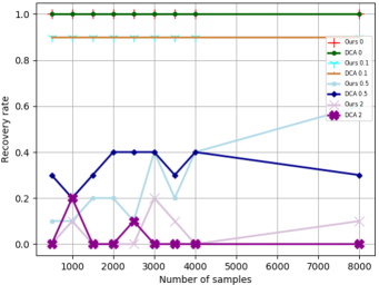
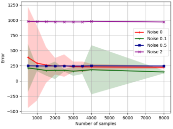
The synthetic data matrix used in the experiments is generated in the form of , where , the entries of noise are generated by sampling Gaussian distribution with noise level , the entries of and are generated by i.i.d. uniform distribution in at first and then their rows are normalized to have unit norm. Analogous to DCA, we use the recovery rate as the metric to evaluate the precision of anchor recovery. The anchor index recovery rate is defined as , where refers to the anchor set obtained by our algorithm or DCA.
We set the dimensions of as and set as 10. We generate four datasets with different noise levels, which are . The number of subproblems is set as . We give nine different settings for the number of sampling for our algorithm, ranging from to . We compare our algorithm with DCA to determine the anchor set . The simulation results are shown in Figure 2. For the case of , both our algorithm and DCA can accurately locate all anchors. With increased noise, the recovery rate continuously decreases both for our algorithm and DCA, since the separability assumption is not preserved. As shown in Figure 2 (b), the reconstruction error, which is evaluated by the Frobenius norm of , continuously decreases with increased for the noiseless case. In addition, the variance of the reconstructed error, illustrated by the shadow region, continuously shrinks with increased . For the high noise level case, the collapsed separability assumption arises that the reconstruction error is unrelated to .
5 Conclusion
In this paper, we have proposed a sublinear runtime classical algorithm to resolve the general minimum conical hull problem. We first reformulated the general minimum conical hull problem as a sampling problem. We then exploited two sampling subroutines and proposed the general heuristic post-selection method to achieve low computational cost. We theoretically analyzed the correctness and the computation cost of our algorithm. The proposed algorithm benefit numerous learning tasks that can be mapped to the general minimum conical hull problem, especially for tasks that need to process datasets on a huge scale. There are two promising future directions. First, we will explore other advanced sampling techniques to further improve the polynomial dependence in the computation complexity. Second, we will investigate whether there exist other fundamental learning models that can be reduced to the general minimum conical hull problem. One of the most strongest candidates is the semi-definite programming solver.
6 Note Added
Recently we became aware of an independent related work [6], which employs the divide-and-conquer anchoring strategy to solve separable nonnegative matrix factorization problems. Since a major application of the general conical hull problem is to solve matrix factorization, their result can be treated as a special case of our study. Moreover, our study adopts more advanced techniques and provides a better upper complexity bounds than theirs.
References
- [1] Esma Aïmeur, Gilles Brassard, and Sébastien Gambs. Quantum clustering algorithms. In Proceedings of the 24th international conference on machine learning, pages 1–8. ACM, 2007.
- [2] Juan Miguel Arrazola, Alain Delgado, Bhaskar Roy Bardhan, and Seth Lloyd. Quantum-inspired algorithms in practice. arXiv preprint arXiv:1905.10415, 2019.
- [3] Mikhail Belkin and Kaushik Sinha. Polynomial learning of distribution families. In 2010 IEEE 51st Annual Symposium on Foundations of Computer Science, pages 103–112. IEEE, 2010.
- [4] Jacob Biamonte, Peter Wittek, Nicola Pancotti, Patrick Rebentrost, Nathan Wiebe, and Seth Lloyd. Quantum machine learning. arXiv preprint arXiv:1611.09347, 2016.
- [5] Christopher M Bishop. Pattern recognition and machine learning. springer, 2006.
- [6] Zhihuai Chen, Yinan Li, Xiaoming Sun, Pei Yuxan, and Jialin Zhang. A quantum-inspired classical algorithm for separable non-negative matrix factorizations. To appear in the Proceedings of the 28th International Joint Conference on Artificial Intelligence.
- [7] Nai-Hui Chia, Tongyang Li, Han-Hsuan Lin, and Chunhao Wang. Quantum-inspired classical sublinear-time algorithm for solving low-rank semidefinite programming via sampling approaches. arXiv preprint arXiv:1901.03254, 2019.
- [8] Nai-Hui Chia, Han-Hsuan Lin, and Chunhao Wang. Quantum-inspired sublinear classical algorithms for solving low-rank linear systems. arXiv preprint arXiv:1811.04852, 2018.
- [9] A. P. Dempster, N. M. Laird, and D. B. Rubin. Maximum likelihood from incomplete data via the EM algorithm. Journal of the Royal Statistical Society: Series B (Methodological), 39(1):1–22, sep 1977.
- [10] Arthur P Dempster, Nan M Laird, and Donald B Rubin. Maximum likelihood from incomplete data via the em algorithm. Journal of the Royal Statistical Society: Series B (Methodological), 39(1):1–22, 1977.
- [11] Chen Ding, Tian-Yi Bao, and He-Liang Huang. Quantum-inspired support vector machine. arXiv preprint arXiv:1906.08902, 2019.
- [12] David Donoho and Victoria Stodden. When does non-negative matrix factorization give a correct decomposition into parts? In Advances in neural information processing systems, pages 1141–1148, 2004.
- [13] Yuxuan Du, Tongliang Liu, Yinan Li, Runyao Duan, and Dacheng Tao. Quantum divide-and-conquer anchoring for separable non-negative matrix factorization. arXiv preprint arXiv:1802.07828, 2018.
- [14] Stuart Geman and Donald Geman. Stochastic relaxation, gibbs distributions, and the bayesian restoration of images. IEEE Transactions on Pattern Analysis and Machine Intelligence, PAMI-6(6):721–741, November 1984.
- [15] Stuart Geman and Donald Geman. Stochastic relaxation, gibbs distributions, and the bayesian restoration of images. In Readings in computer vision, pages 564–584. Elsevier, 1987.
- [16] András Gilyén, Seth Lloyd, and Ewin Tang. Quantum-inspired low-rank stochastic regression with logarithmic dependence on the dimension. arXiv preprint arXiv:1811.04909, 2018.
- [17] Aram W Harrow, Avinatan Hassidim, and Seth Lloyd. Quantum algorithm for linear systems of equations. Physical review letters, 103(15):150502, 2009.
- [18] Roger A Horn and Charles R Johnson. Matrix analysis. Cambridge university press, 2012.
- [19] Ravindran Kannan and Santosh Vempala. Randomized algorithms in numerical linear algebra. Acta Numerica, 26:95–135, 2017.
- [20] Ashish Kapoor, Nathan Wiebe, and Krysta Svore. Quantum perceptron models. In Advances in Neural Information Processing Systems, pages 3999–4007, 2016.
- [21] Iordanis Kerenidis and Anupam Prakash. Quantum recommendation systems. In 8th Innovations in Theoretical Computer Science Conference (ITCS 2017). Schloss Dagstuhl-Leibniz-Zentrum fuer Informatik, 2017.
- [22] Kevin B Korb and Ann E Nicholson. Bayesian artificial intelligence. CRC press, 2010.
- [23] Abhishek Kumar, Vikas Sindhwani, and Prabhanjan Kambadur. Fast conical hull algorithms for near-separable non-negative matrix factorization. In International Conference on Machine Learning, pages 231–239, 2013.
- [24] Neil D Lawrence. Gaussian process latent variable models for visualisation of high dimensional data. In Advances in neural information processing systems, pages 329–336, 2004.
- [25] Daniel D Lee and H Sebastian Seung. Learning the parts of objects by non-negative matrix factorization. Nature, 401(6755):788, 1999.
- [26] Yang Liu and Shengyu Zhang. Fast quantum algorithms for least squares regression and statistic leverage scores. Theoretical Computer Science, 657:38–47, 2017.
- [27] Seth Lloyd, Masoud Mohseni, and Patrick Rebentrost. Quantum algorithms for supervised and unsupervised machine learning. arXiv preprint arXiv:1307.0411, 2013.
- [28] Seth Lloyd, Masoud Mohseni, and Patrick Rebentrost. Quantum principal component analysis. Nature Physics, 10(9):631–633, 2014.
- [29] John C Loehlin. Latent variable models: An introduction to factor, path, and structural analysis. Lawrence Erlbaum Associates, Inc, 1987.
- [30] Andriy Mnih and Ruslan R Salakhutdinov. Probabilistic matrix factorization. In Advances in neural information processing systems, pages 1257–1264, 2008.
- [31] Ruslan Salakhutdinov and Andriy Mnih. Probabilistic matrix factorization. In Proceedings of the 20th International Conference on Neural Information Processing Systems, NIPS’07, pages 1257–1264, USA, 2007. Curran Associates Inc.
- [32] Mikkel N Schmidt, Ole Winther, and Lars Kai Hansen. Bayesian non-negative matrix factorization. In International Conference on Independent Component Analysis and Signal Separation, pages 540–547. Springer, 2009.
- [33] Solomon Eyal Shimony. Finding maps for belief networks is np-hard. Artificial Intelligence, 68(2):399–410, 1994.
- [34] Ewin Tang. A quantum-inspired classical algorithm for recommendation systems. arXiv preprint arXiv:1807.04271, 2018.
- [35] Ewin Tang. Quantum-inspired classical algorithms for principal component analysis and supervised clustering. arXiv preprint arXiv:1811.00414, 2018.
- [36] Aad W Van Der Vaart and Jon A Wellner. Weak convergence. In Weak Convergence and Empirical Processes, pages 16–28. Springer, 1996.
- [37] Nathan Wiebe, Ashish Kapoor, and Krysta Svore. Quantum algorithms for nearest-neighbor methods for supervised and unsupervised learning. arXiv preprint arXiv:1401.2142, 2014.
- [38] Xindong Wu, Xingquan Zhu, Gong-Qing Wu, and Wei Ding. Data mining with big data. IEEE transactions on knowledge and data engineering, 26(1):97–107, 2013.
- [39] Xiyu Yu, Wei Bian, and Dacheng Tao. Scalable completion of nonnegative matrix with separable structure. In Thirtieth AAAI Conference on Artificial Intelligence, 2016.
- [40] Tianyi Zhou, Wei Bian, and Dacheng Tao. Divide-and-conquer anchoring for near-separable nonnegative matrix factorization and completion in high dimensions. In Data Mining (ICDM), 2013 IEEE 13th International Conference on, pages 917–926. IEEE, 2013.
- [41] Tianyi Zhou, Jeff A Bilmes, and Carlos Guestrin. Divide-and-conquer learning by anchoring a conical hull. In Advances in Neural Information Processing Systems, pages 1242–1250, 2014.
We organize the supplementary material as follows. In Section A, we detail the binary tree structure to support length-square sampling operations. We detail the inner product subroutine and the thin matrix-vector multiplication subroutine in Section B. We then provide the proof of Theorem 5 in Section C. Because the proof of Theorem 6 cost employs the results of Theorem 7, we give the proof of Theorem 7 in Section D and leave the proof of Theorem 6 in Section E.
Appendix A The Binary Tree Structure for Length-square Sampling Operations
As mentioned in the main text, a feasible solution to fulfill norm sampling operations is the binary tree structure (BNS) to store data [21]. Here we give the intuition about how BNS constructed for a vector. For ease of notations, we assume the given vector has size with . As demonstrated in Figure 3, the root node records the square norm of . The -th leaf node records the -th entry of and its square value, e.g., . Each internal node contains the sum of the values of its two immediate children. Such an architecture ensures the norm sampling opeartions.
Appendix B Two Sampling Subroutines
Here we introduce two sampling subroutines, the inner product subroutine and the thin matrix-vector multiplication subroutine [34], used in the proposed algorithm.
B.1 Inner product subroutine
In our algorithm, the inner product subroutine is employed to obtain each entry of in parallel, i.e., estimates , where , , and . Let be a random variable that, for , takes value
with probability
| (7) |
We can estimate using as follows [8]. Fix . Let
| (8) |
We first sample the distribution with times to obtain a set of samples , followed by dividing them into groups, , where each group contains samples. Let be the empirical mean of the -th group , and let be the median of . Then [16, Lemma 12] and [8, Lemma 7] guarantee that, with probability at least , the following holds.
| (9) |
The computational complexity of the inner product subroutine is:
Lemma 8 ([16, Lemma 12] and [8, Lemma 7]).
Assume that the overall access to is and the query access to and is and , respectively. The runtime complexity to yield Eqn. (9) is
Proof.
We first recall the main result of Lemma 12 in [16]. Given the overall access to and query access to the matrix and with complexity and , the inner product can be estimated to precision with probability at least in time
With setting the precision to instead of , it can be easily inferred that the runtime complexity to estimate with probability at least is
∎
B.2 Thin matrix-vector multiplication subroutine
Given a matrix and with the norm sampling access, the thin matrix-vector multiplication subroutine aims to output a sample from . The implementation of the thin matrix-vector multiplication subroutine is as follows [16].
For each loop
-
1.
Sample a column index uniformly.
-
2.
Sample a row index from distribution ;
-
3.
Compute
-
4.
Output with probability or restart to sample again (Back to step 1).
We execute the above loop until a sample is successfully output.
The complexity of the thin matrix-vector multiplication subroutine, namely, the required number of loops, is:
Appendix C General Heuristic Post-selection (Proof of Theorem 5)
Recall that the anchor is defined as
The goal of the general heuristic post-selection is approximating by sampling distributions and with times, since the acquisition of the explicit form of and requires computation complexity and collapses the desired speedup. Let be examples independently sampled from with and be the number of examples taking value of with . Similarly, let be examples independently sampled from with and be the number of examples taking value of with . Denote that is the total number of different indexes after sampling with times, and are two indexes corresponding to the -th largest value among and with and , respectively222Due to the limited sampling times, the sampled results (or ) may occupy a small portion of the all (or ) possible results.. Similarly, denote that is the total number of distinguished indexes after sampling with times, the indexes and are -th largest value among and with and , respectively. In particular, we have
The procedure of the general heuristic post-selection is as follows.
-
1.
Sample with times and order the sampled items to obtain with ;
-
2.
Query the distribution to obtain the value with ;
-
3.
Sample with times and order the sampled items to obtain with .
-
4.
Locate with and .
An immediate observation is that, with , we have , where
The general heuristic post-selection is guaranteed by the following theorem (the formal description of Theorem 5).
Theorem 10 ((Formal) General heuristic post-selection).
Assume that and are multinomial distributions. If , and for the constants and with , then for any , and , we have with a probability at least .
Remark. The physical meaning of can be treated as the threshold of the ‘near-anchor’, that is, when the distance of a data point and the anchor point after projection is within the threshold , we say the data point can be treated as anchors. The real anchor set therefore should be expanded and include these near anchors. In other words, and can be manually controllable. The parameter is bounded as follows.
In this work, we set and , which gives .
An equivalent statement of Theorem 10 is:
Problem 11.
How many samples, and , are required to guarantee and , where and .
Lemma 12 (Breteganolle-Huber-Carol inequality [36]).
Let be a multinomial distribution with event probabilities . We randomly sample events from and let be the number of event appeared. Then, the following holds with a probability at least for any ,
| (10) |
Proof of Theorem 10.
The proof is composed of two parts. The first part is to prove that the index with can be determined with sampling complexity . The second part is to prove that the index with can be determined with sampling complexity .
For the first part, we split the set into two subsets and , i.e., and . The decomposition of into two subsets is equivalent to setting in Eqn. (10). In particular, we have and . The Breteganolle-Huber-Carol inequality yields
| (11) |
The above inequality implies that, when , we have
| (12) | |||||
| (13) |
with probability at least .
The assumption guarantees that by sampling with times. In addition, since we have assumed that , it can be easily inferred that, when with a probability at least , there is one and only one value that is in the -neighborhood of . We therefore conclude that can be guaranteed by sampling with .
For the second part, we split the set into three subsets , and , i.e., , , and . Analogous to the above case, the decomposition of into three subsets for the case of sampling is equivalent to setting in Eqn. (10). In particular, we have , , and . The Breteganolle-Huber-Carol inequality yields
| (14) |
The above inequality implies that, when , we have
| (15) |
with probability at least .
Since we have assumed , we have . In other words, guarantees that by sampling with times. In addition, the assumption leads to that, when with a probability at least , there is one and only one value that is in the -neighborhood of . We therefore conclude that with .
Combing the results of two parts together, it can be easily inferred that, with the sampling complexity , we have with probability . ∎
Appendix D Proof of Theorem 7
In this section, we give the proof of Theorem 7. We left the detailed proof of Theorem 14 and 15 in subsection D.1 and D.2, respectively.
Proof of Theorem 7.
Recall that , and is an approximation of . The triangle inequality yields
| (16) |
where is the total variation distance of . In the following, we bound the two terms on the right-hand side of Eqn. (16) respectively.
Correctness of . The goal here is to prove that
| (17) |
By Lemma 13 below, Eqn (17) follows if the following inequality holds:
| (18) |
Finally, the inequality in Eqn. (18) is guaranteed to hold because of Theorem 14.
Lemma 13 (Lemma 6.1, [34]).
For satisfying , the corresponding distributions and satisfy .
Theorem 14.
Let the rank and the condition number of be and , respectively. Fix
Then, Algorithm 2 yields with probability at least .
Correctness of . Analogous to the above part, we bound
| (19) |
to yield
| (20) |
And Eqn. (19) can be obtained by the following theorem.
Theorem 15.
Let the rank of be . Set the number of samplings in the inner product subroutine as
Then, Algorithm 2 yields with at least success probability.
D.1 Proof of Theorem 14
Due to , we have
| (21) | |||||
where and is the left singular vectors of . The first inequality of Eqn. (21) is obtained by exploiting the submultiplicative property of spectral norm [18], i.e., for any matrix and any vector , we have . The second inequality of Eqn. (21) comes from the submultiplicative property of spectral norm and . To achieve in Eqn. (18), Eqn. (21) indicates that the approximated left singular matrix should satisfy
| (22) |
The spectral norm can be quantified as:
Theorem 16.
Suppose that the rank of is , and refers to a approximated singular vector of such that
| (23) |
Then, we have
| (24) |
Theorem 16 implies that to achieve Eqn. (22) (or equivalently, Eqn. (18)), we should bound as
| (25) |
We use the following lemma to give an explicit representation of by the sampled matrix and ,
Lemma 17.
Suppose that refers to the right singular vector of such that and , where . Suppose that the rank of both and is and
Let , then we have
| (26) |
In conjunction with Eqn. (23) and Eqn. (26), we set and rewrite Eqn. (25) as
| (27) |
In other words, when , Eqn. (18) is achieved so that . Recall that is quantified by as defined in Eqn. (26), we use the following theorem to bound , i.e.,
Theorem 18.
Given a nonnegative matrix , let , be the sampled matrix following Algorithm 1. Setting as , with probability at least , we always have ,
Combining the result of Theorem 16 and Lemma 17, we know that with sampling rows of , the approximated distribution is -close to the desired result, i.e.,
D.1.1 Proof of Theorem 16
We first introduce a lemma to facilitate the proof of Theorem 16, i.e.,
Lemma 19 (Adapted from Lemma 5, [16]).
Let be a matrix of rank at most , and suppose that has columns that span the row and column spaces of . Then .
Proof of Theorem 16.
The main procedure to prove this theorem is as follows. By employing the Lemma 19, we can set and as
and then bound and separately. Lastly, we combine the two results to obtain the bound in Eqn. (24).
Following the above observation, we first bound the term . We rewrite as
| (28) |
The entry of with is bounded by , i.e.,
| (29) |
The first equivalence of Eqn. (D.1.1) comes from the definition of , and the second equivalence employs The first inequality of Eqn. (D.1.1) exploits triangle inequality and Eqn. (23), i.e.,
| (30) |
The second inequality of Eqn. (D.1.1) directly comes from the triangle inequality. The last second inequality of Eqn. (D.1.1) employs the inequality for both the case and , guaranteed by Eqn. (23) and . Specifically, for the case , we bound as
For the case , we bound as
The last inequality of Eqn. (D.1.1) comes from
since
D.1.2 Proof of Lemma 17
Proof of Lemma 17.
The inequality in Eqn. (26) can be proved following the definition of . Mathematically, we have
| (32) |
The first equivalence of Eqn. (D.1.2) comes from the definition of . The first inequality of Eqn. (D.1.2) is derived by employing , i.e.,
| (33) |
The last second equivalence of Eqn. (D.1.2) employs
The last inequality of Eqn. (D.1.2) uses
∎
D.1.3 Proof of Theorem 18
We introduce the following lemma to facilitate the proof.
Lemma 20 (Adapted from Theorem 4.4, [19]).
Given any matrix . Let be obtained by length-squared sampling with . Then, for all , we have
| (34) |
Hence, for , with probability at least we have .
D.2 Proof of Theorem 15
Proof of Theorem 15.
We first give the upper bound of the term , i.e.,
| (37) |
The first inequality comes from the the submultiplicative property of spectral norm. The second inequality supported by Eqn. (27) with
Following the definition of norm, we have
Denote the additive error
we rewrite Eqn. (37) as
| (38) |
An observation of the above equation is that we have if
| (39) |
Appendix E The Complexity of The Algorithm (Proof of Theorem 6)
Proof of Theorem 6.
As analyzed in the main text, the complexity of the proposed algorithm is dominated by four operations in the preprocessing step and the divide step, i.e., finding the left singular vectors , estimating the inner product to build , preparing the approximated probability distribution , and estimating the rescale factor . We evaluate the computation complexity of these four operations separately and then give the overall computation complexity of our algorithm.
In this subsection, we first evaluate the computation complexity of these four parts separately and then combine the results to give the computation complexity of our algorithm. Due to same reconstruction rule, we use a general setting that can either be or to evaluate the computation complexity for the four parts.
Complexity of Finding . Supported by the norm sampling operations, the matrix can be efficiently constructed following Algorithm 1, where query complexity is sufficient. Applying SVD onto with generally costs
runtime complexity. Once we obtain such the SVD result of , the approximated left singular vectors can be implicitly represented, guaranteed by the following Lemma:
Lemma 21 (Adapted from [34]).
Let the given dataset support the norm sampling operations along with the description of , We can sample from any in expected queries with and query for any particular entry in queries.
Complexity of Estimating by . The runtime complexity to estimate by obeys the following corollary, i.e.,
Corollary 22.
Let be the input vector, be the input matrix with rank , and be the approximated left singular matrix. We can estimate by to precision with probability at least using
runtime complexity.
Proof of Corollary 22.
Theorem 15 indicates that, to estimate by , the required number of samplings is
Following the result of Lemma 8, the runtime complexity to obtain is
| (41) |
Since for any indicated by Eqn. (37), we rewrite Eqn. (41) as
| (42) |
We now quantify the access cost of , and to give an explicit bound of Eqn. (41). We have and , since and are stored in BNS data structure. We have supported by Lemma 21. Combing the above access cost and Eqn. (41), the runtime complexity to estimate is
Since each entry can be computed in parallel, the runtime complexity to obtain is also
∎
Complexity of Sampling from . Recall that the definition of is . We first evaluate the computation complexity to obtain one sample from . From Lemma 9, we know the expected runtime complexity to sample from is . Specifically, we have
| (43) |
where the first inequality employs the triangle inequality, the second inequality employs the submultiplicative property of spectral norm, and the third inequality utilizes with . Concurrently, we have . Employing Lemma 21 to quantify and , the complexity to obtain a sample from is
With substituting with its explicit representation in Theorem 7, the complexity is
Following the result of the general heuristic post-selection method in Theorem 10, we sample the distribution with times in parallel, which gives the runtime complexity
Complexity of estimating by . For the general case with , we should estimate the norm of their project results, i.e., that can either be or . Recall that the explicit representation of the approximated result is with , where the -th entry of is and the else entries are zero. An immediate observation is that can be obtained by using the inner product subroutine in Lemma 8.
We first calculate the sample and query complexity to query the -th entry of , namely, the query and sample complexity to obtain the inner product of . By employing the result of the inner product subroutine, with removing and setting both and as , we can estimate to precision with probability at least in time
| (44) |
where we use Lemma 21 to get and the inequality comes from in Eqn. (21). We store nonzero entries of in memory.
We next use the inner product subroutine to obtain with . Since both and are stored in memory, we have and . Following the result of Lemma 8, we can estimate to precision with probability at least with runtime complexity
| (45) |
The overall complexity of our algorithm. An immediate observation of the above four parts is that the query complexity and runtime complexity of our algorithm is denominated by the complexity of finding , i.e., . Since is a general setting that can either be or , the runtime complexity for our algorithm is
∎