Subspace Determination through
Local Intrinsic Dimensional Decomposition:
Theory and Experimentation

Abstract

Axis-aligned subspace clustering generally entails searching through enormous numbers of subspaces (feature combinations) and evaluation of cluster quality within each subspace. In this paper, we tackle the problem of identifying subsets of features with the most significant contribution to the formation of the local neighborhood surrounding a given data point. For each point, the recently-proposed Local Intrinsic Dimension (LID) model is used in identifying the axis directions along which features have the greatest local discriminability, or equivalently, the fewest number of components of LID that capture the local complexity of the data. In this paper, we develop an estimator of LID along axis projections, and provide preliminary evidence that this LID decomposition can indicate axis-aligned data subspaces that support the formation of clusters.

1 Introduction

In data mining, machine learning, and other areas of AI, we are often faced with datasets that contain many more attributes than needed, or that can even be helpful for tasks such as clustering or classification. Problems associated with such high dimensional data are for example the concentration effect of distances [13, 20] or irrelevant features [25, 49]. For clustering [31] and outlier detection [49], researchers have made use of various techniques to identify relevant subspaces, as defined by subsets of features that are informative for a particular task. Examples of how relevant subspaces can be determined for individual clusters or outliers include local density estimation in a systematic search through candidate subspaces (often following the Apriori principle [7] in various adaptations to the subspace search problem [48]), or the adaptation of distance measures based on the distribution within local neighborhoods (using some analysis of variance or even covariance — typically based on PCA — to allow also for an adaptation to correlated features). For sufficiently tight local neighborhoods, the underlying local data manifold can be regarded as approaching a linear form [40], an assumption that further justifies the determination of locally relevant features for subspace determination.

In this paper, we present a novel technique for the identification of subsets of features with the most significant contribution to the formation of the local neighborhood surrounding a given data point, using the recently introduced Local Intrinsic Dimensionality (LID) [22, 23] model. LID is a distributional form of intrinsic dimensional modeling in which the volume of a ball of radius $r$ is taken to be the probability measure associated with its interior, denoted by $F(r)$. The function $F$ can be regarded as the cumulative distribution function (cdf) of an underlying distribution of distances. Theoretical properties of LID in multivariate analysis have been studied recently [24]. LID has also seen practical applications in such areas as similarity search [16], dependency analysis [39], and deep learning [33, 34].

To make use of the LID model to identify locally-discriminative features, we develop an estimator of LID decomposed along axis projections that compensates for the bias introduced during projection. We also provide preliminary experimental evidence that LID decomposition can indicate axis-aligned data subspaces that support the formation of clusters, by implementing a simple two-stage technique whereby points are first assigned to relevant subspaces, and then clustered. As the relevant features can be different for each cluster, feature relevance is assessed cluster-wise or even point-wise (as the clusters are not known in advance). It is not our intent here to propose a complete subspace clustering strategy; rather the goal in this preliminary investigation is to provide some guidance as to how subspace identification could be done as an independent, initial step as part of a larger clustering strategy.

In the remainder of the paper, after giving a short overview of existing work in subspace clustering (Section 2) and preliminaries from the literature on intrinsic dimensionality (Section 3), we discuss the formal theory of decomposition of LID across features (Section 4), and the practical estimation of the decomposed LID (Section 5). To illustrate how LID decomposition could be used within subspace clustering, we propose as an example a simple method using LID to determine eligible subspaces within which DBSCAN is used for clustering (Section 6). We conclude the paper with discussion of other potential use cases (Section 7).

2 Related Work

Subspace clustering [32, 42] aims at finding clusters defined in subspaces or projections of the original dataspace. The relevant features can be different for each cluster, and feature relevance is assessed cluster-wise or even point-wise (as the clusters are not known in the beginning of the process). The typical approach is to ignore or downweight those features that are not contributing to the formation of the given cluster. This differs from global feature selection, which applies the same feature weighting to all clusters.

As typical algorithmic approaches to the problem, we can distinguish bottom-up versus top-down procedures [31]. Subspace clustering aims at finding all clusterings in all (relevant) subspaces while projected clustering aims at finding one clustering solution where each cluster can reside in a subspace (projection) that is different from the other clusters’ subspace. Top-down procedures (typically solving the projected clustering problem) start in the full dimensional space with some proto-cluster [5, 45, 46, 18], or local neighborhood point set [14, 21], and derive some adaptive weighting of distances for the clustering procedure. Bottom-up procedures start in one-dimensional subspaces associated with single features, and then iteratively combine those features deemed relevant or interesting, assessing the importance of the feature for proto-clusters in subspaces [6, 17, 37, 29, 9, 10] or for the local neighborhoods of individual points [47, 30, 2, 4, 3, 35]. As testing all combinations would lead to an exponentially-large search space, these approaches typically identify some monotonic property that allows early pruning of less-promising combinations following principles borrowed from frequent pattern mining [48]. Even so, existing subspace clustering methods remain computationally expensive, and tend to deliver many redundant subspaces and clusters.

Some methods consider feature combinations directly or assess (linear) correlations among features. These typically rely on locally applied PCA as a primitive to assess locally relevant feature combinations [15, 4] or on an adaptation of the Hough transform [1], which is computationally even more expensive.

3 Preliminaries

Let $X\in\mathbb{R}^{m}$ be an $m$-variate random variable, let $F:\mathbb{R}^{m}\rightarrow\mathbb{R}$ be its joint probability distribution, and let $\|\cdot\|$ denote an arbitrary norm. The local intrinsic dimensionality and indiscriminability of $F$ at a non-zero point $x$ are defined as follows.

Definition 1 ([24])

Let $x\in\mathbb{R}_{\neq 0}^{m}$ such that $F(x)\neq 0$.

1. The intrinsic dimensionality of $F$ at $x$ is defined as

   $$\operatorname{IntrDim}_{F}(x) := \lim_{\varepsilon\to 0}\frac{\ln(F((1+\varepsilon)x)/F(x))}{\ln(1+\varepsilon)}.$$

2. The indiscriminability of $F$ at $x$ is defined as

   $$\operatorname{InDiscr}_{F}(x) := \lim_{\varepsilon\to 0}\frac{F((1+\varepsilon)x)-F(x)}{\varepsilon\cdot F(x)}.$$

3. If the partial derivatives $\frac{\partial f}{\partial x_{i}}(x)$ at $x$ exist for all $i\in[m]=\{1,\ldots,m\}$, the $\operatorname{ID}$ of $F$ at $x$ is defined as

   $$\operatorname{ID}_{F}(x):=\frac{x^{T}\nabla F(x)}{F(x)}.$$

The following theorem (see [24] for the proof) yields the equivalence of the above three concepts under suitable conditions.

Theorem 1 ([24])

Let $x\in\mathbb{R}_{\neq 0}^{m}$. If there exists an open interval $I\subseteq\mathbb{R}$ with $0\in I$ such that $F$ is non-zero and its partial derivatives exist and are continuous at $(1+\varepsilon)x$ for all $\varepsilon\in I$, then

$$\operatorname{ID}_{F}(x)=\operatorname{IntrDim}_{F}(x)=\operatorname{InDiscr}_{F}(x).$$

Local intrinsic dimensionalities have also been shown to satisfy the following useful decomposition rule.

Theorem 2 ([24])

Let $x\in\mathbb{R}_{\neq 0}^{m}$ and let $I\subseteq\mathbb{R}$ with $0\in I$ be an open interval such that $F$ is non-zero and its partial derivatives exist and are continuous at $(1+\varepsilon)x$ for all $\varepsilon\in I$. Assume that $x_{i}\neq 0$ for each $i\in[m]$. Then

$$\operatorname{ID}_{F}(x) =\sum_{i=1}^{m}\operatorname{ID}_{F_{i,x}}(x_{i}),$$

where we define $F_{i,x}(t):=F(x_{1},\ldots,x_{i-1},t,x_{i+1},\ldots,x_{m})$ for every $i\in[m]$.

4 LID Decomposition

4.1 Moore-Osgood Theorem

We recall the following classical result from multivariate mathematical analysis, often referred to as the Moore-Osgood Theorem (for a reference, see for example [28]). For a subset $X\subset M$ of a metric space $M$, let us denote by $\bar{X}$ the set of limit points of $X$.

Theorem 3 (Moore-Osgood)

Let $M_{1}$, $M_{2}$, and $M$ be metric spaces, respectively, let $f:A\times B\to M$ be a function from a subset $A\times B\subset M_{1}\times M_{2}$ into $M$ and let $x_{0}\in\bar{A}$ and $y_{0}\in\bar{B}$. If

1. $\psi(y):=\lim_{x\to x_{0}}f(x,y)$ exists for each $y\in B$, and

2. $\phi(x):=\lim_{y\to y_{0}}f(x,y)$ exists uniformly in $x\in A$,

then the following three limits are all guaranteed to exist and are equal: $\lim_{x\to x_{0}}\lim_{y\to y_{0}}f(x,y)$, $\lim_{y\to y_{0}}\lim_{x\to x_{0}}f(x,y)$, and $\lim_{(x,y)\to(x_{0},y_{0})}f(x,y)$.

Note: The notation $\lim_{(x,y)\to(x_{0},y_{0})}f(x,y)=L$ is shorthand for the following statement:

For all $\varepsilon>0$, there exists $\delta>0$ such that $d(f(x,y),L)\leq\varepsilon$ if $d_{1}(x,x_{0})\leq\delta$ and $d_{2}(y,y_{0})\leq\delta$, where $d$, $d_{1}$, and $d_{2}$ denote the metrics of $M$, $M_{1}$, and $M_{2}$, respectively.

In the case of $M$, $M_{1}$, and $M_{2}$ being cross products of $\mathbb{R}$, and the distance metric defined using the Euclidean norm (as $d(x,y):=\|x-y\|$), the above statement can be rewritten as:

For all $\varepsilon>0$, there exists $\delta>0$ such that $\|f(x,y)-L\|\leq\varepsilon$ if $\|(x,y)-(x_{0},y_{0})\|\leq\delta$, where $\|\cdot\|$ denotes the Euclidean norm.

4.2 Definition and Properties

We now define $N_{\delta}:=\{x\in\mathbb{R}^{m}:0<\|x\|_{\infty}<\delta\}$, and assume that $F$ is non-zero and that its partial derivatives exist and are continuous at every $x\in N_{\delta}$. Under this assumption, we note that for every $x\in N_{\delta}$, there exists an interval $I$ with $0\in I$ such that $F$ is non-zero and its partial derivatives exist and are continuous at $(1+\varepsilon)x$ for every $\varepsilon\in I$. Following [24],

$$\operatorname{ID}_{F}^{*}:=\lim_{\begin{smallmatrix}x\to 0\\ \|x\|_{\infty}\leq\delta\end{smallmatrix}}\operatorname{ID}_{F}(x).$$

is defined as the local intrinsic dimensionality of $F$.

Definition 2

Let $I_{\delta}$ be the ‘hollow’ open interval $(-\delta,\delta)\setminus\{0\}$. For $x\in N_{\delta}$, we define the functions $F_{i,x}:I_{\delta}\to\mathbb{R}$ and $g_{i}:I_{\delta}\times{I_{\delta}}^{m-1}\to\mathbb{R}$ as

$$F_{i,x}(t) :=F(x_{1},\ldots,x_{i-1},t,x_{i+1},\ldots,x_{m})\quad\text{ and }\quad$$

$$g_{i}(t,x_{-i}) :=\frac{t\cdot F_{i,x}^{\prime}(t)}{F_{i,x}(t)},$$

where $x_{-i}=(x_{1},\ldots,x_{i-1},x_{i+1},\ldots,x_{m})\in{I_{\delta}}^{m-1}$ for some $x\in N_{\delta}$.

Using the Moore-Osgood theorem to interchange the order of limits, we obtain a decomposition rule for LID.

Theorem 4

Assume that for every $i\in[m]$, it holds that

1. $\lim_{t\to 0}g_{i}(t,y)$ exists for every $y\in{I_{\delta}}^{m-1}$

2. $\lim_{y\to 0}g_{i}(t,y)$ exists for every $t\in I_{\delta}$,

and that at least one of the two limits exists uniformly. Then the limits $\operatorname{ID}_{F,i}^{*}:=\lim_{x\to 0}x_{i}\cdot F_{i,x}^{\prime}(x_{i})/F_{i,x}(x_{i})$ exist for all $i\in[m]$, and thus

$$\begin{split}\operatorname{ID}_{F}^{*}&=\sum_{i=1}^{m}\operatorname{ID}_{F,i}^{*}=\sum_{i=1}^{m}\lim_{x\to 0}\frac{x_{i}\cdot F_{i,x}^{\prime}(x_{i})}{F_{i,x}(x_{i})}=\sum_{i=1}^{m}\lim_{y\to 0}\lim_{t\to 0}g_{i}(t,y).\end{split}$$ (1)

We refer to $\operatorname{ID}_{F,i}^{*}$ as the local intrinsic dimensionality of $F$ in the direction of the $i$-th coordinate.

4.3 Estimating $\operatorname{ID}_{F,i}^{*}$

We begin by making use of the following theorem for the univariate case. We omit the proof and refer the reader to [23].

Theorem 5 ([23])

Let $\phi:\mathbb{R}\to\mathbb{R}$, and assume that $\operatorname{ID}_{\phi}^{*}:=\operatorname{ID}_{\phi}(0)=\lim_{t\to 0}t\cdot\phi^{\prime}(t)/\phi(t)$ exists. Let $t$, $w$ be such that both $t/w$ and $\phi(t)/\phi(w)$ are positive. If $\phi$ is non-zero and continuously differentiable everywhere in $[\min\{t,w\},\max\{t,w\}]$, then

$$\frac{\phi(t)}{\phi(w)}=\Big{(}\frac{t}{w}\Big{)}^{\operatorname{ID}^{*}_{\phi}}\cdot G_{\phi,w}(t),$$

where $G_{\phi,w}(t):=\exp\left(\int_{t}^{w}\frac{\operatorname{ID}_{\phi}^{*}-\operatorname{ID}_{\phi}(\theta)}{\theta}d\theta\right)$. Moreover, if there is an open interval containing 0 on which $\phi$ is non-zero and continuously differentiable, except perhaps at 0 itself, then, for any fixed $c>1$, it holds that

$$\lim_{\begin{smallmatrix}w\to 0^{+}\\ 1/c\leq t/w\leq c\end{smallmatrix}}G_{\phi,w}(t)=\lim_{\begin{smallmatrix}w\to 0^{-}\\ 1/c\leq t/w\leq c\end{smallmatrix}}G_{\phi,w}(t)=1.$$

Note that the above theorem implies that as $w$ approaches 0 either from above or below, it holds that $\phi(t)\approx\phi(w)\cdot(t/w)^{\operatorname{ID}^{*}_{\phi}}$. Moreover, differentiating this quantity yields $(\phi(w)/w)\cdot\operatorname{ID}^{*}_{\phi}\cdot(t/w)^{\operatorname{ID}^{*}_{\phi}-1}$ as an approximation of $\phi^{\prime}(t)$.

We now turn to the estimation of $\operatorname{ID}_{F,i}^{*}$ for some $i\in[m]$. Let us fix some $x\in\mathbb{R}_{\neq 0}^{m}$ and let us denote $\operatorname{ID}_{i}^{*}:=\operatorname{ID}_{F_{i,x}}^{*}$ for $i\in[m]$. Given $p^{(1)},\ldots,p^{(k)}\in\mathbb{R}^{m}$ following the joint distribution $F$, we are now in a position to state the log-likelihood function for the parameter $\operatorname{ID}_{i}^{*}$ under the observations $p^{(1)},\ldots,p^{(k)}$. Assume that we associate a weight $\omega(p^{(j)}_{i})$ to the projection $p^{(j)}_{i}$ of each observation $p^{(j)}$ — for the standard unweighted case of the log-likelihood function, all weights are set to 1. We may regard these weights as assigning a-priori likelihoods to the observations, by which an individual observation $p^{(j)}_{i}$ is accounted as having occurred $\omega(p^{(j)}_{i})$-many times. The weighted log-likelihood function can then be derived as

$$\mathcal{L}(\operatorname{ID}_{i}^{*}:p^{(1)},\ldots,p^{(k)}) = \sum_{j=1}^{k}\omega\left(p^{(j)}_{i}\right)\cdot\log\left(\frac{F_{i,x}(w)}{w}\cdot\operatorname{ID}_{i}^{*}\cdot\left(\frac{|p^{(j)}_{i}|}{w}\right)^{\operatorname{ID}_{i}^{*}-1}\right)$$

$$= \left(\log\left(\frac{F_{i,x}(w)}{w}\right)+\log\left(\operatorname{ID}_{i}^{*}\right)\right)\cdot\left(\sum_{j=1}^{k}\omega\left(p^{(j)}_{i}\right)\right)$$

$$\hskip 71.13188pt+\left(\operatorname{ID}_{i}^{*}-1\right)\cdot\sum_{j=1}^{k}\omega\left(p^{(j)}_{i}\right)\cdot\log\left(\frac{\left|p^{(j)}_{i}\right|}{w}\right).$$

We are now interested in the parameter $\operatorname{ID}_{i}^{*}$ that maximizes $\mathcal{L}(\operatorname{ID}_{i}^{*}:p^{(1)},\ldots,p^{(k)})$. For this purpose, we form the derivative of $\mathcal{L}(\operatorname{ID}_{i}^{*}:p^{(1)},\ldots,p^{(k)})$ with respect to $\operatorname{ID}_{i}^{*}$ and set it to zero. A straightforward derivation shows that the likelihood is maximized at

$$\frac{\Big{(}\sum_{j=1}^{k}\omega\left(p^{(j)}_{i})\right)}{\widehat{\operatorname{ID}_{i}^{*}}}+\sum_{j=1}^{k}\omega\left(p^{(j)}_{i}\right)\cdot\log\left(\frac{\left|p^{(j)}_{i}\right|}{w}\right)=0\,,$$

or equivalently,

$$\widehat{\operatorname{ID}_{i}^{*}}=\left(-\frac{1}{\sum_{j=1}^{k}\omega\left(p^{(j)}_{i}\right)}\sum_{j=1}^{k}\omega\left(p^{(j)}_{i}\right)\log\left(\frac{\left|p^{(j)}_{i}\right|}{w}\right)\right)^{-1},$$ (2)

which has the form of a weighted variant of the Hill estimator with threshold $w$.

Note that we have now developed an estimator for $\operatorname{ID}_{i}^{*}$. Assuming however, that for a reference point $x_{0}\in\mathbb{R}^{m}$, the considered neighborhood from which the points $p^{(1)},\ldots,p^{(k)}$ are chosen is sufficiently small, it is reasonable to use the same estimator for $\operatorname{ID}_{F,i}^{*}$ as well, as the outer limit in (1) can be neglected.

Figure 1: Consider a circular neighborhood of a reference point $x_{0}$ in two dimensions, where the reference point is shifted to the origin and the neighborhood is scaled by $\max\{\|p^{(j)}\|_{\infty}:j\in[k]\}$. Due to the circular form, points $p$ with projections $|p_{i}|$ close to one are much less likely than points with projections close to zero. This is because points in the blue region have not been taken into account. It may seem like the most appropriate choice for the neighborhood when estimating the values of $\operatorname{ID}_{i}^{*}$ is the rectilinear neighborhood given by the infinity norm. It turns out however, that a Euclidean-distance neighborhood can be employed provided that we adjust for bias, by associating weights $\omega(p_{1})=1/(1-|p_{1}|^{2})^{1/2}$ to the projection $p_{1}$ of the observation $p$. The weight $\omega(p_{1})$ associated with $p$ is proportional to 1 over the length of the line segment that contains all points with this projection $|p_{1}|$. In spaces of arbitrary dimension $m$, the weight of an observation point $p_{i}$, when estimating $\operatorname{ID}_{F,i}^{*}$ must be proportional to $\pi^{(m-1)/2}(1-|p_{i}|^{2})^{(m-1)/2}/\Gamma((m{+}1)/2)$, the ratio of the volume of the unit cube (1) and the volume of the $(m{-}1)$-dimensional sphere with radius $(1-|p_{i}|^{2})^{1/2}$.

4.4 Neighborhood Weighting

In the previous subsection, we have developed an estimator for $\operatorname{ID}_{F,i}^{*}$; however, we have not yet stated how to determine a neighborhood for $x_{0}$. This turns out to be a delicate question, for which the use of observation weighting will become essential.

Note that the estimator for $\operatorname{ID}_{F,i}^{*}$ that we developed above assumes that neighborhood points $p^{(j)}$ with projections $|p_{j}|$ stem from the interval $[0,w]$. If we pick a ‘box neighborhood’ of $x_{0}$ consisting of the $k$ closest points to $x_{0}$ with respect to the $L_{\infty}$ norm (defined as $\|v\|_{\infty}:=\max\{|v_{i}|:i\in[m]\}$ for $v\in\mathbb{R}^{m}$), the points $p$ with projections $|p_{i}|$ close to zero are equally likely to be neighbors as points with projections close to one. This is however, not the case if we pick the neighborhood as the $k$ closest points with respect to the Euclidean norm. In this case, points $p$ with projections $|p_{i}|$ close to zero will be much more likely to be neighbors than points with $|p_{i}|$ close to one. However, the Euclidean norm is much more common in practical applications, due to its rotational invariance.

In order to compensate for the bias that results from the fact that points with large projections are less likely than points with small projection when employing the Euclidean norm, we will use the weighting scheme introduced in the previous subsection. When estimating $\operatorname{ID}_{F,i}^{*}$, an observation $p$ with projection $|p_{i}|$ must be weighted according to the ratio of the volume of the $m-1$-dimensional sphere with radius $(1-|p_{i}|^{2})^{1/2}$ on the one hand, and the volume of its bounding hypercube on the other. This leads to the definition of weights $\omega(p_{i}):=1/(1-|p_{i}|^{2})^{(m-1)/2}$ for the case of the Euclidean norm. See Figure 1 for an illustration of the two-dimensional case.

5 Experimental Analysis

In this section, we provide some experimental evidence of the effectiveness of the developed estimators, by testing on certain synthetic data classes.

Verifying $\operatorname{ID}_{F}^{*}=\sum_{i=1}^{m}\operatorname{ID}_{F,i}^{*}$.

In the first experiment, we experimentally verify the equation $\operatorname{ID}_{F}^{*}=\sum_{i=1}^{m}\operatorname{ID}_{F,i}^{*}$ from Theorem 4 for the case of a uniform distribution in a space equipped with the Euclidean distance metric. For the purpose of estimating $\operatorname{ID}_{F}^{*}$, we use the MLE (Hill) estimator proposed in [8]. Given a reference point $x_{0}$, this estimator assumes a neighborhood of the $k$ closest points, and returns the value

$$\widehat{\operatorname{ID}_{F}^{*}}=\left(-\frac{1}{k}\sum_{j=1}^{k}\log\Bigg{(}\frac{\|p^{(j)}-x_{0}\|}{w}\Bigg{)}\right)^{-1}.$$

Here, $w$ is chosen as the maximum distance of any neighborhood point $p^{(j)}$ from the reference point $x_{0}$. We call this estimator hill_distances.

Figure 2: Plot for the results for estimators hill_distances, sum_hill_projections, and sum_w_hill_projections in a neighborhood of size $k=100$, for dimensions $m$ between $2$ and $1024$. Note that the neighborhoods for hill_distances and sum_w_hill_projections are chosen with respect to the Euclidean norm, while the neighborhoods for sum_hill_projections are chosen with respect to the $L_{\infty}$ norm. The errorbars denote 95% confidence intervals with every measurement being the average of 5 runs.

We compare this value $\widehat{\operatorname{ID}_{F}^{*}}$ with the sum $\sum_{i=1}^{m}\widehat{\operatorname{ID}_{i}^{*}}$, where we consider two ways of obtaining the estimates $\widehat{\operatorname{ID}_{i}^{*}}$. In the first case (sum_hill_projections), we pick $k$ nearest neighbors with respect to the $L_{\infty}$ norm. In the second case (sum_w_hill_projections), we use the weighted estimator for the Euclidean norm, as described above, with compensation for bias using weights as defined in Section 4.4.

In our experiment, we create a uniform neighborhood of $k=100$ points within radius 1 of the reference point (chosen to be the origin) for increasing dimensions $m=2,4,8,\ldots,1024$. For the hill_distances and sum_w_hill_projections estimators, we create a hyperspherical ($L_{2}$-norm) $k$-neighborhood. Note that rejection sampling fails to construct this neighborhood when $m$ is large, due to the extremely high rejection rates. Instead, it is necessary to use a method for generating uniformly distributed points on a sphere based on a normal distribution, as for example described in [36]. For the sum_hill_projections-estimator, we create a hypercubical ($L_{\infty}$) neighborhood of radius 1, and evaluate the estimator as in (2), with all weights set to one. The results can be found in Figure 2. Note that in this example of a uniform distribution in $m$ dimensions, the true LID value is $m$. The experiments show that the two decomposition-based estimators, when summed over all components, do match the total intrinsic dimensionality $m$, as does the MLE estimator.

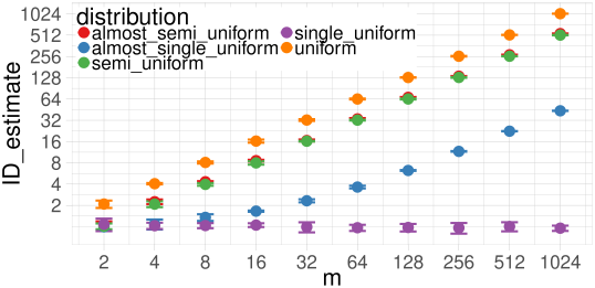
Figure 3: ID estimates as they were computed by sum_hill_projections in an $L_{\infty}$ neighborhood of $k=100$ points, for different combinations of uniform distributions.

Estimating ID values for different combinations of uniform distributions.

We evaluate the results that sum_hill_projections gives for different combinations of uniform distributions. We create $L_{\infty}$ $100$-neighborhoods for the following distributions:

uniform

refers to the uniform distribution in $m$ dimensions with radius 1.

single_uniform

denotes the distribution that is uniform with radius $1$ only in the first dimension, and set to $0$ in the remaining $m-1$ dimensions.

semi_uniform

denotes a distribution that is uniform with radius $1$ in the first $m/2$ dimensions, and set to $0$ for the remaining $m/2$ dimensions.

almost_single_uniform

denotes the distribution that is uniform with radius $1$ only in the first dimension, and uniform with radius $10^{-10}$ in the remaining $m-1$ dimensions.

almost_semi_uniform

denotes a distribution that is uniform with radius $1$ in the first $m/2$ dimensions, and uniform with radius $10^{-10}$ in the remaining $m/2$ dimensions.

Otherwise, the parameter choices are identical to those of the previous experiment. We can see the results in Figure 3. As expected, the intrinsic dimensionalities of the semi_uniform and single_uniform distributions are estimated to be approximately $m/2$ and $1$, respectively. Interestingly, but not surprisingly, the almost_single_uniform case, the addition of small amounts of uniform noise in all but the first coordinate eventually overcomes the contribution of the first coordinate, as $m$ increases. All measurements are averages over 5 runs, and the error bars indicate 95% confidence intervals.

6 Subspace Clustering Based on LID Decomposition

We now consider some of the issues surrounding the use of LID-decomposition ranking to support subspace clustering. It is not our intent here to propose a single full subspace clustering strategy; rather, the goal is to provide some guidance as to how subspace identification could be done as an independent, preliminary step as part of a larger clustering strategy.

The main idea is to rely on the LID decomposition to determine relevant attributes for the cluster to which the neighborhood of $q$ belongs. The subspace dimensionality of a point $q$ is determined by searching for attributes with low $\mathrm{ID}$ estimates. One well-recognized way of doing this is by locating a gap in the sequence of LID estimates that best separates relevant attributes from irrelevant ones, much in the same way as a projective basis is found in PCA decompositions through gaps in the sequence of eigenvalues or variances.

Definition 3

Relative Difference Let $\mathcal{W}(q)$ be a set with $\mathrm{ID}_{\mathcal{A}_{i}}$ in the neighborhood of $q$ in ascending order. The relative difference is defined as:

$$\Delta^{k}_{r}(q)=(\mathcal{W}_{k+1}(q)-\mathcal{W}_{k}(q))/{\mathcal{W}_{k+1}(q)}$$

We track the relative difference in $\mathrm{ID}$ from attributes with low $\mathrm{ID}$ to high $\mathrm{ID}$ and fix the cut-off that determines the subspace dimensionality at the attribute that exhibits the highest relative difference. We give a pseudo code description in Algorithm 1.

Input: Query point $q\in\mathcal{X}$, Set of attributes $\mathcal{A}=\{\mathcal{A}_{i}\mid i\in\mathbb{N}^{d}\}$.

Output: A subspace preference vector $\mathcal{S}(q)$.

1 Get the $k$-nearest-neighbors $p$ of $q$ w.r.t. the infinity norm;

2

3for $\mathcal{A}_{i}\in\mathcal{A}$ do

4       Get projections $p^{i}$ of $p$ in $\mathcal{A}_{i}$;

5       Calculate $\widehat{ID}^{*}$;

6       Assign $\mathcal{W}_{i}(q)\leftarrow\widehat{ID}^{*}$;

7      

8 end for

9Sort $\mathcal{W}(q)$ in ascending order, and return ordered vector of attributes $\mathcal{O}(q)$;

10 Calculate relative ID differences $\Delta^{k}_{r}(q)$ (Def. 3);

11 Determine the position $\alpha$ at which a gap is detected in terms of relative ID difference: $\alpha=\operatorname*{arg\,max}_{i\in[m]}\Delta^{k}_{r}(q)$;

Return subspace preference vector with dimensionality $\alpha$: $\mathcal{S}(q)=\{\mathcal{O}_{i}(q)\mid i=1,..,\alpha\}$.

Algorithm 1 Determine a subspace preference vector for a query point.

6.1 Subspace Membership

To better define the local subspace preference vectors, we propose an additional refinement step. We use a sample of data points $\tilde{\mathcal{X}}$ to build a profile from their subspace preference vectors $\mathcal{P}=\{\mathcal{S}(x)\mid x\in\tilde{\mathcal{X}}\}$. The local subspace preference is refined by determining the membership of points $\mathcal{M}$ to the collected subspace profiles. Given the ordered attributes vector $\mathcal{O}(q)$, $\mathcal{M}(q)$ is selected as the subspace which attributes are present in the first elements of $\mathcal{O}(q)$. When the profiles are ordered from low to high dimensional subspaces, this selection process naturally follows the monotonicity rule in assigning membership to higher dimensional subspaces in cases where the point belongs to a higher dimensional cluster.

The approach described so far (see Algorithm 2) determines the membership of a point to a detected subspace without defining the relationship among the points with the same subspace membership. Inside a subspace, points with preference towards that subspace are clustered using a traditional algorithm such as DBSCAN [19].

Input: Query point $q\in\mathcal{X}$, Ordered set of attributes $\mathcal{O}(q)$, Subspace profiles $\mathcal{P}$.

Output: Subspace membership $\mathcal{M}(q)$.

1 Sort $\mathcal{P}$ in ascending order according to the dimension of the subspace;

2

3for $\nu\in\mathcal{P}$ do

4       Set $\mu=dim(\nu)$;

5       if $\nu\subseteq\mathcal{O}^{\mu}$ s.t. $\mathcal{O}^{\mu}=\{\mathcal{O}_{1},...,\mathcal{O}_{\mu}\}$ then

6             $\mathcal{M}(q)=\nu$.

7       end if

8      

9 end for

Algorithm 2 Refine membership to a subspace profile.

6.2 Experimental Evaluation

Besides the recall, we rely on three other metrics that are widely used in the literature to measure the performance of clustering techniques, namely the Adjusted Rand-Index (ARI) [27], the Normalized Mutual Information (NMI) [43], and the Adjusted Mutual Information (AMI) [44].

6.2.1 Low-dimensional Data

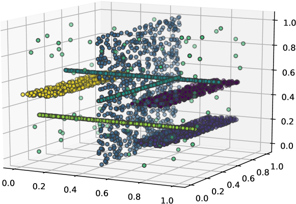
Figure 4: DiSH 3D Dataset.

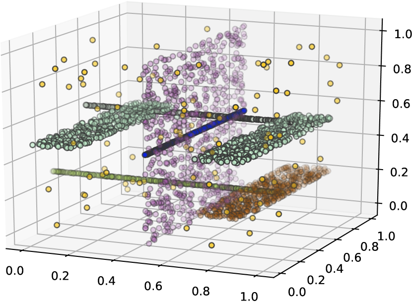
(a) DiSH

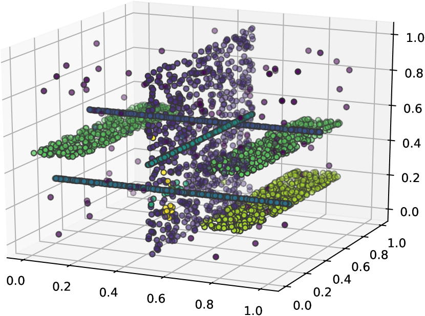
(b) LID-DBSCAN

Figure 5: Clustering results on the DiSH 3D dataset shown in Figure 4.

	NMI	AMI	ARI	Recall
DiSH	0.943	0.891	0.879	0.872
LID-DBSCAN	0.918	0.894	0.921	0.952

Table 1: Clustering performance on the DiSH 3D dataset shown in Figure 4.

We start our validation with the low dimensional illustrative dataset used in the original DiSH publication [3], shown here in Figure 4. The dataset contains 3D points grouped in a hierarchy of 1D and 2D subspace clusters with several inclusions and additional noise points. Figure 5 shows the results of clustering this set with the carefully tuned DiSH parameters $\epsilon=0.005$ and $\mu=150$, as well as our approach with a neighborhood size $k=100$ and $\rho=0$.

Table 1 summarizes the clustering performance. We can see that our approach slightly improves over DiSH, especially in terms of recall.

6.2.2 Higher-dimensional data

We synthetically generated three datasets (T1, T2, T3) with $30$, $50$, and $100$ attributes, respectively, each consisting of 5 standard Gaussian clusters with each attribute value from a given cluster generated according to $\mathcal{N}(c,r)$, with $c$ and $r$ having been selected uniformly at random from $[{-1},1]$ and $(0,0.2]$, respectively. For T1 and T2, each cluster was generated in its own distinct subspace (with no attributes in common between clusters). For the purpose of studying the resilience of the approach to noise, the data was augmented with attributes whose values were drawn uniformly at random from $[{-1},1]$. T3 was generated from T2 by adding 50 additional attributes with uniform noise. The details are summarized in Table 6(a). Table 6(b) summarizes the clustering performance for these datasets comparing our approach against DiSH [3] and CLIQUE [6]. We chose DiSH as it also relies on a point-wise determination of relevant attributes (essentially comparing the spread of distances of nearest neighbors in all attributes) and could be seen as closely related to our approach. In addition, we test against the classical method CLIQUE, as it is arguably the best-known subspace clustering method. In most cases, our approach shows a superior performance in detecting the correct subspaces and clusterings.

(a) Description.

	$d$	$||\mathcal{S}||$	Noisy $\mathcal{A}_{i}$
T1	30	$\{5,5,5,5,5\}$	5
T2	50	$\{3,5,7,7,11\}$	17
T3	100	$\{3,5,7,7,11\}$	67

(b) Results.

		NMI	AMI	ARI	Recall
T1	DiSH	0.535	0.362	0.264	0.582
	CLIQUE	0.431	0.275	0.303	0.635
	LID-DBSCAN	0.801	0.734	0.803	0.726
T2	DiSH	0.568	0.396	0.532	0.7
	CLIQUE	0.644	0.473	0.568	0.78
	LID-DBSCAN	0.779	0.695	0.716	0.765
T3	DiSH	0.570	0.397	0.412	0.702
	CLIQUE	0.644	0.473	0.568	0.78
	LID-DBSCAN	0.749	0.671	0.699	0.76

Table 2: Toy datasets.

6.3 Manifold Data

For the purpose of further validating the efficiency of the approach to detect significant subspaces on more complex datasets, we relied on the manifold generator proposed in [41], which generated manifolds of differing distributions in different dimensions. In our experiments, we built four different datasets that merge a subset of these manifolds to study the behavior of the algorithm. D1 contains mostly relatively low dimensional manifolds and one high dimensional non-linear manifold. D2 is similar to D1 in which the non-linear manifold has been replaced by a Gaussian cluster. Low and high dimensional manifolds were used to build D3 and D4 respectively. The details of the datasets are summarized in Table 3. The approach performance is compared against that of DiSH. The choice of DiSH is motivated by its modularity, and its similar approach to subspace clustering in which the algorithm can be divided into two subroutines: one for subspace detection, and a second for clustering points by identifying memberships embedded in hierarchical clusters. These subroutines are executed sequentially, which makes it possible to use only the first module to compare the performances of both approaches at subspace detection. A parameter tuning was performed for DiSH in which the 30 best performing configurations were chosen.

(a) Manifolds

#	$d$	Description
$m_{1}$	11	Uniformly sampled sphere
$m_{2}$	5	Affine space
$m_{3}$	6	Concentrated figure
		confusable with a 3d one
$m_{4}$	8	Non-linear manifold
$m_{5}$	3	2-d helix
$m_{6}$	36	Non-linear manifold
$m_{7}$	3	Swiss roll
$m_{8}$	72	Non-linear manifold
$m_{9}$	20	Affine space
$m_{10}$	11	Uniformly sampled hypercube
$m_{11}$	3	Mobius band 10-times twisted
$m_{12}$	20	Isotropic multivariate Gaussian
$m_{13}$	13	Curve

(b) Datasets

#	$d$	Manifold subset
D1	78	$\{m_{3},m_{6},m_{7},m_{9},m_{13}\}$
D2	62	$\{m_{3},m_{7},m_{9},m_{12},m_{13}\}$
D3	41	$\{m_{2},m_{3},m_{4},m_{5},m_{7},m_{11},m_{13}\}$
D4	76	$\{m_{6},m_{9},m_{12}\}$

Table 3: Synthetic manifolds and datasets

Since we are concerned with the efficiency of the approach to detect relevant subspaces, metrics that are generally used to judge the goodness-of-fit of clustering algorithms, especially those defined for subspace clustering, can not be employed. For example, instead of detecting a set of objects and attributes, subspace detection is concerned with detecting a subset of objects that determine the preference of an object to a subset of attributes. That being said, taking into consideration this definition, one metric can be adapted from subspace clustering evaluation to subspace detection. In addition, we develop a different metric that is more relevant to the locality assumption of our study.

• The Relative Non-Intersecting Area (RNIA)[38] measures to which extent the found subspaces cover the true subspaces. Best performance would detect all true features, and only these features. To achieve this, the union set $U$ is defined as consisting of those elements present in both the true subspaces and the predicted subspaces. Similarly, the intersection set $I$ is defined to consist of those features that are common to both the true and predicted subspaces. For the purposes of our evaluation, we will take RNIA to be the complement of its usual definition:

  $$\mathit{RNIA}=1-(|U|-|I|)/|U|=|I|/|U|\,.$$

• Average Relative Relevance (ARR). The RNIA measure defined above is strict in that it considers all features. Alternatively, we can measure the extent to which the local subspace preference detection is efficient in detecting the most relevant features, regardless of the complete true feature vector. We define the ARR to be the average number of detected true features:

  $$\mathit{ARR}=\frac{1}{N}\sum_{i=0}^{N}\frac{I_{i}}{S_{i}},$$

  where $S_{i}$ is the subspace preference vector for point $p_{i}$, and $I_{i}$ the intersection between $S_{i}$ and the true subspace vector.

The experimental outcomes for DiSH and the LID decomposition approach are shown in Figure 8. With respect to both RNIA and ARR, LID decomposition significantly outperforms DiSH for each of the 4 datasets considered, particularly for D4 (the set with highest average manifold dimension).

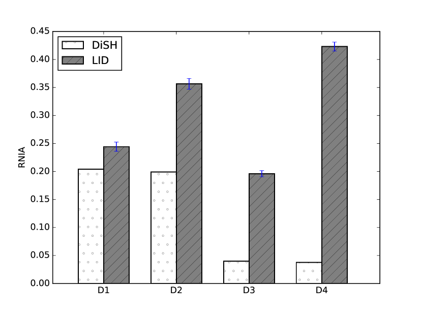
(a) RNIA

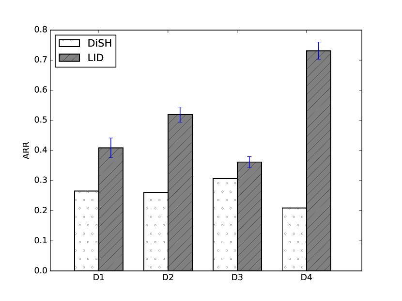
(b) ARR

Figure 8: Subspace detection performance for DiSH and the LID-based approach.

7 Conclusion

In this preliminary work, we studied the decomposition of local intrinsic dimensionality (LID), the estimation of decomposed LID, and a practical simple application example of the decomposed LID for subspace clustering. The results of the experimental comparison with DiSH show the potential for the use of decomposition of LID for identifying important features for subspace clustering prior to the performance of the clustering itself.

Using decomposed LID as a new primitive for estimating the local relevance of a feature, future work could explore more refined subspace clustering approaches. Clustering approaches can be tailored to this new primitive but presumably many existing subspace clustering methods could be adapted to using the new primitive instead of conventional building blocks such as density-estimates, analysis of variance, or distance distributions. Beyond subspace clustering, many more applications can be envisioned, for example in subspace outlier detection [49] or in subspace similarity search [12, 26].

Variance-based measures of feature relevance, such as those underlying PCA and its variants, have an advantage over LID in that sample variances decompose perfectly across the coordinates within a Euclidean space. However, although the theoretical values within an LID decomposition are guaranteed to be additive, their estimates are not. Although the experimental results shown in Figure 2 indicate for the case of uniform distributions that MLE estimates for decomposed LID do sum to the overall LID estimate within reasonable tolerances, it is not clear how well additivity is conserved for real data. Since the additivity of estimators for LID decomposition may depend significantly on their accuracy, future research in this area could benefit from the further development of LID estimators of good convergence properties.

Acknowledgments

M. E. Houle was supported by JSPS Kakenhi Kiban (B) Research Grant 18H03296.

References

- [1] Achtert, E., Böhm, C., David, J., Kröger, P., Zimek, A.: Global correlation clustering based on the Hough transform. Stat. Anal. Data Min. 1(3), 111–127 (2008)
- [2] Achtert, E., Böhm, C., Kriegel, H.P., Kröger, P., Müller-Gorman, I., Zimek, A.: Finding hierarchies of subspace clusters. In: Proc. PKDD. pp. 446–453 (2006)
- [3] Achtert, E., Böhm, C., Kriegel, H.P., Kröger, P., Müller-Gorman, I., Zimek, A.: Detection and visualization of subspace cluster hierarchies. In: Proc. DASFAA. pp. 152–163 (2007)
- [4] Achtert, E., Böhm, C., Kriegel, H.P., Kröger, P., Zimek, A.: Robust, complete, and efficient correlation clustering. In: Proc. SDM. pp. 413–418 (2007)
- [5] Aggarwal, C.C., Procopiuc, C.M., Wolf, J.L., Yu, P.S., Park, J.S.: Fast algorithms for projected clustering. In: Proc. SIGMOD. pp. 61–72 (1999)
- [6] Agrawal, R., Gehrke, J., Gunopulos, D., Raghavan, P.: Automatic subspace clustering of high dimensional data for data mining applications. In: Proc. SIGMOD. pp. 94–105 (1998)
- [7] Agrawal, R., Srikant, R.: Fast algorithms for mining association rules. In: Proc. VLDB. pp. 487–499 (1994)
- [8] Amsaleg, L., Chelly, O., Furon, T., Girard, S., Houle, M.E., Kawarabayashi, K., Nett, M.: Estimating local intrinsic dimensionality. In: Proc. KDD. pp. 29–38 (2015)
- [9] Assent, I., Krieger, R., Müller, E., Seidl, T.: DUSC: dimensionality unbiased subspace clustering. In: Proc. ICDM. pp. 409–414 (2007)
- [10] Assent, I., Krieger, R., Müller, E., Seidl, T.: EDSC: efficient density-based subspace clustering. In: Proc. CIKM. pp. 1093–1102 (2008)
- [11] Becker, R., Hafnaoui, I., Houle, M.E., Li, P., Zimek, A.: Subspace determination through local intrinsic dimensional decomposition. In: Proc. SISAP (2019)
- [12] Bernecker, T., Emrich, T., Graf, F., Kriegel, H.P., Kröger, P., Renz, M., Schubert, E., Zimek, A.: Subspace similarity search: Efficient -NN queries in arbitrary subspaces. In: Proc. SSDBM. pp. 555–564 (2010)
- [13] Beyer, K., Goldstein, J., Ramakrishnan, R., Shaft, U.: When is “nearest neighbor” meaningful? In: Proc. ICDT. pp. 217–235 (1999)
- [14] Böhm, C., Kailing, K., Kriegel, H.P., Kröger, P.: Density connected clustering with local subspace preferences. In: Proc. ICDM. pp. 27–34 (2004)
- [15] Böhm, C., Kailing, K., Kröger, P., Zimek, A.: Computing clusters of correlation connected objects. In: Proc. SIGMOD. pp. 455–466 (2004)
- [16] Casanova, G., Englmeier, E., Houle, M., Kröger, P., Nett, M., Schubert, E., Zimek, A.: Dimensional testing for reverse -nearest neighbor search. PVLDB 10(7), 769–780 (2017)
- [17] Cheng, C.H., Fu, A.W.C., Zhang, Y.: Entropy-based subspace clustering for mining numerical data. In: Proc. KDD. pp. 84–93 (1999)
- [18] Domeniconi, C., Papadopoulos, D., Gunopulos, D., Ma, S.: Subspace clustering of high dimensional data. In: Proc. SDM (2004)
- [19] Ester, M., Kriegel, H.P., Sander, J., Xu, X.: A density-based algorithm for discovering clusters in large spatial databases with noise. In: Proc. KDD. pp. 226–231 (1996)
- [20] François, D., Wertz, V., Verleysen, M.: The concentration of fractional distances. IEEE TKDE 19(7), 873–886 (2007)
- [21] Friedman, J.H., Meulman, J.J.: Clustering objects on subsets of attributes. J. R. Statist. Soc. B 66(4), 825–849 (2004)
- [22] Houle, M.E.: Dimensionality, discriminability, density and distance distributions. In: Proc. ICDM Workshops. pp. 468–473 (2013)
- [23] Houle, M.E.: Local intrinsic dimensionality I: an extreme-value-theoretic foundation for similarity applications. In: Proc. SISAP. pp. 64–79 (2017)
- [24] Houle, M.E.: Local intrinsic dimensionality II: multivariate analysis and distributional support. In: Proc. SISAP. pp. 80–95 (2017)
- [25] Houle, M.E., Kriegel, H.P., Kröger, P., Schubert, E., Zimek, A.: Can shared-neighbor distances defeat the curse of dimensionality? In: Proc. SSDBM. pp. 482–500 (2010)
- [26] Houle, M.E., Ma, X., Oria, V., Sun, J.: Efficient algorithms for similarity search in axis-aligned subspaces. In: Proc. SISAP. pp. 1–12 (2014)
- [27] Hubert, L., Arabie, P.: Comparing partitions. J. Classif. 2(1), 193–218 (1985)
- [28] Kadelburg, Z., Marjanović, M.: Interchanging two limits. The Teaching of Mathematics 8(1), 15–29 (2005)
- [29] Kailing, K., Kriegel, H.P., Kröger, P.: Density-connected subspace clustering for high-dimensional data. In: Proc. SDM. pp. 246–257 (2004)
- [30] Kriegel, H.P., Kröger, P., Renz, M., Wurst, S.: A generic framework for efficient subspace clustering of high-dimensional data. In: Proc. ICDM. pp. 250–257 (2005)
- [31] Kriegel, H.P., Kröger, P., Zimek, A.: Clustering high dimensional data: A survey on subspace clustering, pattern-based clustering, and correlation clustering. ACM TKDD 3(1), 1–58 (2009)
- [32] Kriegel, H.P., Kröger, P., Zimek, A.: Subspace clustering. WIREs DMKD 2(4), 351–364 (2012)
- [33] Ma, X., Li, B., Wang, Y., Erfani, S.M., Wijewickrema, S.N.R., Schoenebeck, G., Song, D., Houle, M.E., Bailey, J.: Characterizing adversarial subspaces using local intrinsic dimensionality. In: Proc. ICLR. pp. 1–15 (2018)
- [34] Ma, X., Wang, Y., Houle, M.E., Zhou, S., Erfani, S.M., Xia, S., Wijewickrema, S.N.R., Bailey, J.: Dimensionality-driven learning with noisy labels. In: Proc. ICML. pp. 3361–3370 (2018)
- [35] Moise, G., Sander, J., Ester, M.: Robust projected clustering. KAIS 14(3), 273–298 (2008)
- [36] Muller, M.E.: A note on a method for generating points uniformly on n-dimensional spheres. Commun. ACM 2(4), 19–20 (Apr 1959)
- [37] Nagesh, H.S., Goil, S., Choudhary, A.: Adaptive grids for clustering massive data sets. In: Proc. SDM. pp. 1–17 (2001)
- [38] Patrikainen, A., Meila, M.: Comparing subspace clusterings. IEEE Transactions on Knowledge and Data Engineering 18(7), 902–916 (2006)
- [39] Romano, S., Chelly, O., Nguyen, V., Bailey, J., Houle, M.E.: Measuring dependency via intrinsic dimensionality. In: ICPR16. pp. 1207–1212 (Dec 2016)
- [40] Roweis, S.T., Saul, L.K.: Nonlinear dimensionality reduction by locally linear embedding. Science 290, 2323–2326 (2000)
- [41] Rozza, A., Lombardi, G., Ceruti, C., Casiraghi, E., Campadelli, P.: Novel high intrinsic dimensionality estimators. Machine learning 89(1-2), 37–65 (2012)
- [42] Sim, K., Gopalkrishnan, V., Zimek, A., Cong, G.: A survey on enhanced subspace clustering. Data Min. Knowl. Disc. 26(2), 332–397 (2013)
- [43] Strehl, A., Ghosh, J.: Cluster ensembles – a knowledge reuse framework for combining multiple partitions. J. Mach. Learn. Res. 3, 583–617 (2002)
- [44] Vinh, N.X., Epps, J., Bailey, J.: Information theoretic measures for clustering comparison: Variants, properties, normalization and correction for chance. J. Mach. Learn. Res. 11, 2837–2854 (2010)
- [45] Woo, K.G., Lee, J.H., Kim, M.H., Lee, Y.J.: FINDIT: a fast and intelligent subspace clustering algorithm using dimension voting. Inform. Software Technol. 46(4), 255–271 (2004)
- [46] Yip, K.Y., Cheung, D.W., Ng, M.K.: On discovery of extremely low-dimensional clusters using semi-supervised projected clustering. In: Proc. ICDE. pp. 329–340 (2005)
- [47] Yiu, M.L., Mamoulis, N.: Iterative projected clustering by subspace mining. IEEE TKDE 17(2), 176–189 (2005)
- [48] Zimek, A., Assent, I., Vreeken, J.: Frequent pattern mining algorithms for data clustering. In: Aggarwal, C.C., Han, J. (eds.) Frequent Pattern Mining, chap. 16, pp. 403–423. Springer (2014)
- [49] Zimek, A., Schubert, E., Kriegel, H.P.: A survey on unsupervised outlier detection in high-dimensional numerical data. Stat. Anal. Data Min. 5(5), 363–387 (2012)